Wind, waves, and surface currents in the Southern Ocean: observations from the Antarctic Circumnavigation Expedition
←
→
Page content transcription
If your browser does not render page correctly, please read the page content below
Earth Syst. Sci. Data, 13, 1189–1209, 2021
https://doi.org/10.5194/essd-13-1189-2021
© Author(s) 2021. This work is distributed under
the Creative Commons Attribution 4.0 License.

            Wind, waves, and surface currents in the Southern
                 Ocean: observations from the Antarctic
                     Circumnavigation Expedition
          Marzieh H. Derkani1 , Alberto Alberello2,3 , Filippo Nelli1 , Luke G. Bennetts3 , Katrin G. Hessner4 ,
            Keith MacHutchon5 , Konny Reichert6 , Lotfi Aouf7 , Salman Khan8 , and Alessandro Toffoli1
      1 Department   of Infrastructure Engineering, The University of Melbourne, 3010, Melbourne, Victoria, Australia
                                2 Department of Physics, University of Turin, 10125, Turin, Italy
           3 School of Mathematical Sciences, University of Adelaide, 5005, Adelaide, South Australia, Australia
                                        4 OceanWaveS GmbH, 21339 Lüneburg, Germany
                5 Department of Civil Engineering, University of Cape Town, 7701, Cape Town, South Africa
                                     6 Independent Scholar, 6021 Wellington, New Zealand
                                            7 Météo-France, 31100, Toulouse, France
                  8 Oceans and Atmosphere, Commonwealth Scientific and Industrial Research Organisation,

                                               3195, Aspendale, Victoria, Australia
                      Correspondence: Marzieh H. Derkani (marzieh.h.derkani@gmail.com) and
                                    Alessandro Toffoli (toffoli.alessandro@gmail.com)
                                 Received: 27 August 2020 – Discussion started: 17 October 2020
                       Revised: 6 February 2021 – Accepted: 12 February 2021 – Published: 22 March 2021

      Abstract. The Southern Ocean has a profound impact on the Earth’s climate system. Its strong winds, in-
      tense currents, and fierce waves are critical components of the air–sea interface and contribute to absorbing,
      storing, and releasing heat, moisture, gases, and momentum. Owing to its remoteness and harsh environment,
      this region is significantly undersampled, hampering the validation of prediction models and large-scale ob-
      servations from satellite sensors. Here, an unprecedented data set of simultaneous observations of winds, sur-
      face currents, and ocean waves is presented, to address the scarcity of in situ observations in the region –
      https://doi.org/10.26179/5ed0a30aaf764 (Alberello et al., 2020c) and https://doi.org/10.26179/5e9d038c396f2
      (Derkani et al., 2020). Records were acquired underway during the Antarctic Circumnavigation Expedition
      (ACE), which went around the Southern Ocean from December 2016 to March 2017 (Austral summer). Ob-
      servations were obtained with the wave and surface current monitoring system WaMoS-II, which scanned the
      ocean surface around the vessel using marine radars. Measurements were assessed for quality control and com-
      pared against available satellite observations. The data set is the most extensive and comprehensive collection
      of observations of surface processes for the Southern Ocean and is intended to underpin improvements of wave
      prediction models around Antarctica and research of air–sea interaction processes, including gas exchange and
      dynamics of sea spray aerosol particles. The data set has further potentials to support theoretical and numerical
      research on lower atmosphere, air–sea interface, and upper-ocean processes.

Published by Copernicus Publications.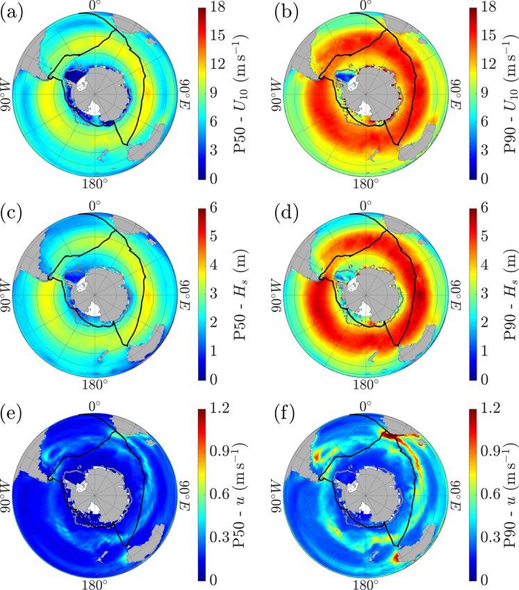
1190                                                        M. H. Derkani et al.: Sea state observations in the Southern Ocean

1   Introduction                                                     2019), measurements have primarily been taken en route to
                                                                     Antarctic stations, leaving entire sectors undersampled. Fur-
The Southern Ocean comprises an uninterrupted band of                ther, measurements normally concentrate on the lower at-
water around Antarctica south of the 60th parallel. More             mosphere and/or the upper ocean (not necessarily concomi-
broadly, it refers to the body of water south of the main            tantly), while waves are generally not monitored. Only a
landmasses of Africa, Australia, and South America, with             handful of buoys have operated in the region: (i) the South-
a northern limit at approximately 40◦ S (see, for example,           ern Ocean Flux Station (Schulz et al., 2011, 2012), a me-
Young et al., 2020). This region is dominated by strong              teorological buoy first deployed in 2010 at approximately
westerly winds, the notorious roaring forties, furious fifties,      350 nautical miles south-west of Tasmania (Australia) that
and screaming sixties (Lundy, 2010). They fuel the Antarc-           provides observations of meteorological parameters, includ-
tic Circumpolar Current (the world’s largest ocean current,          ing the directional wave spectrum, downwelling radiation,
e.g. Park et al., 2019), which mixes warm waters descending          and seawater temperature and salinity; (ii) the Southern
from the Atlantic, Indian, and Pacific oceans with northward         Ocean wave buoy network, which is comprised of one direc-
cold streams from the Antarctic. Above all, intense winds            tional wave buoy deployed south of Campbell Island (New
give rise to some of the fiercest waves on the planet (e.g           Zealand) and five drifting buoys (Barbariol et al., 2019); and
Barbariol et al., 2019; Vichi et al., 2019; Young and Ribal,         (iii) the Global Southern Ocean Array and the Global Argen-
2019; Young et al., 2020). Acting as an interface between the        tine Basin Array, which are networks of fixed and moored
lower atmosphere and the upper ocean, waves entrap and re-           platforms and mobile profilers (gliders) deployed south-west
lease momentum, heat, moisture, and gases through breaking           of Chile and in the Argentinian basin, respectively, to mon-
(Melville, 1996; Csanady, 2001; Veron, 2015) and drive air–          itor waves, air–sea fluxes of heat, moisture and momentum,
sea fluxes (e.g. Humphries et al., 2016; Schmale et al., 2019;       and physical, biological, and chemical properties throughout
Thurnherr et al., 2020). Due to almost unlimited fetches (the        the water column (Trowbridge et al., 2019). Buoys have also
distance of open water over which the wind blows), Southern          been deployed in the Antarctic marginal ice zone to moni-
Ocean waves are normally long and fast moving, allowing              tor waves in ice and sea ice drift (e.g. Meiners et al., 2016;
them to inject turbulent motion throughout the water column          Ackley et al., 2020; Meylan et al., 2014; Vichi et al., 2019;
down to depths of 100–150 m, i.e. approximately half wave-           Alberello et al., 2020a).
length, and contributing to ocean mixing (Babanin, 2006;                A database covering the Southern Ocean more uniformly
Qiao et al., 2016; Toffoli et al., 2012; Alberello et al., 2019b).   is provided by polar-orbiting microwave radar satellites such
The combined effect of the Antarctic Circumpolar Current,            as altimeters, scatterometers, and synthetic aperture radar
which cools and sinks near-surface water, and waves, which           (SAR). Nevertheless, sea state observations are scattered in
regulate fluxes and stir the upper ocean, produces a well-           both space and time due to the nature of polar satellite orbits,
mixed layer that extends from about 100 m in the summer              and normally limited to average wind and current speeds, and
months to approximately 500 m in the winter months (e.g.             wave heights. SAR technology provides images that can be
Dong et al., 2008). This deep mixed layer gives the Southern         converted into directional wave energy spectra (Khan et al.,
Ocean capacity to store more heat and gases than any other           2020a). However, SAR only detects swell systems, i.e. long-
latitude band on the planet, making this remote ocean a major        wave systems no longer under the effect of local winds and
driver of the Earth’s climate system (see, for example, Dong         with wavelengths longer than 115 m (Collard et al., 2009). It
et al., 2007).                                                       does not resolve the wind sea, i.e. the short-wave components
   South of the 60th parallel, a strong sea ice seasonal cy-         directly generated by local winds. This limitation is partly ad-
cle of advance and retreat (Eayrs et al., 2019) forms an in-         dressed by the recently launched Chinese-French Oceanog-
tegral part of a coupled atmosphere–sea-ice–ocean system             raphy Satellite (CFOSAT) mission, which detects wave sys-
and influences Southern Ocean dynamics. Sea ice extent               tems with wavelengths longer than 70 m (Hauser et al., 2020;
around Antarctica impacts albedo, atmospheric and thermo-            Aouf et al., 2020).
haline circulation, and ocean productivity (Perovich et al.,            The scarcity of in situ observations has a negative feed-
2008; Massom and Stammerjohn, 2010; Notz, 2012), con-                back on the satellite network, which cannot rely on suffi-
tributing to the heat balance. Further, it attenuates waves,         cient ground truth to be validated with high confidence. In
modulating air–sea fluxes and mixing (Thomas et al., 2019).          turn, this drawback impacts prediction models, which are im-
In turn, waves (in combination with wind) have a significant         paired by notable biases in the Southern Ocean (see, for ex-
feedback to the Antarctic sea ice state, extent, and thickness       ample, Yuan, 2004; Li et al., 2013; Zieger et al., 2015). To
(e.g Wadhams, 1986; Bennetts et al., 2017; Alberello et al.,         address the lack of in situ observations and support calibra-
2019a; Vichi et al., 2019; Alberello et al., 2020a).                 tion and validation of satellite sensors and prediction models,
   In situ observations of atmospheric and oceanographic             an international initiative, organised by the Swiss Polar Insti-
properties are scarce due to the remoteness of the region.           tute, led an unprecedented circumnavigation of the Antarctic
Although there have been many expeditions crossing the               continent (the Antarctic Circumnavigation Expedition, ACE;
Southern Ocean (see a general overview in Schmale et al.,            Walton and Thomas, 2018) during the Austral summer of

Earth Syst. Sci. Data, 13, 1189–1209, 2021                                           https://doi.org/10.5194/essd-13-1189-2021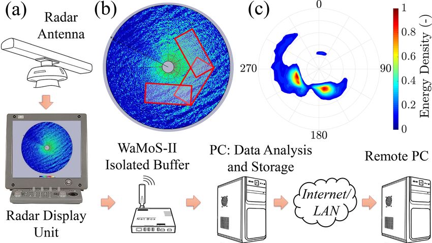
M. H. Derkani et al.: Sea state observations in the Southern Ocean                                                          1191

2016–2017. The objective of the expedition was to sample
concomitant processes in the lower atmosphere, at the ocean
surface, and in the upper-ocean layers all around the Antarc-
tic continent in a single season (Rodríguez-Ros et al., 2020;
Schmale et al., 2019; Smart et al., 2020; Thurnherr et al.,
2020). Here we present a database of underway sea state ob-
servations, comprising of concurrent records of winds, sur-
face currents, and waves. In Sects. 2 and 3, details of the
expedition, the instrumentation, and its calibration are pre-
sented. An overview of the database is presented in Sect. 4.
A comparison against available satellite data and an assess-
ment of uncertainties is given in Sect. 5. Concluding remarks
are made in the last section.

2     The Antarctic Circumnavigation Expedition

ACE took place from 20 December 2016 to 19 March 2017,
encompassing the entire Austral summer. It consisted of a         Figure 1. Map of the ACE voyage divided by legs. Average sea ice
voyage around the Southern Ocean between 34◦ and 74◦ S            concentration during the expedition is also shown.
aboard the Russian research icebreaker Akademik Tryosh-
nikov (see technical details in Walton and Thomas, 2018).
   The voyage was divided into three legs. Leg 1 was along        band radar (9.41 GHz) – a standard equipment on any vessels
the Indian Ocean from Cape Town, South Africa, to Ho-             – to acquire high-definition radar images of the surrounding
bart, Australia, with stops at Marion Island, Iles de Crozet et   ocean surface and derive the directional wave energy spec-
Kerguelen, and Heard Island. Leg 2 went across the Pacific        trum, related integral parameters such as the significant wave
Ocean to Punta Arenas, Chile, with stations at Mertz Glacier,     height and mean wave period, and surface current speed and
Balleny Islands, Scott Island, Mount Siple (the southernmost      direction. Performance of WaMoS-II and its limitations are
station), Peter I Island, and Diego Ramírez. Leg 3 crossed the    discussed in Hessner et al. (2002), Hessner et al. (2008),
Atlantic Ocean back to Cape Town via South Georgia, South         Hessner et al. (2019), Lund et al. (2015a), and Lund et al.
Sandwich Islands, and Bouvetøya. In addition, scientific ob-      (2015b). A summary of the range and accuracy of measured
servations were carried out during transit across the Atlantic    parameters is reported in Appendix A.
on the way to/from South Africa (legs 0 and 4, respectively).        The overall system consists of an A/D converter, a PC,
   A schematic of the expedition is presented in Fig. 1 and       and a processing software connected to the X-band radar (a
photos of the environmental conditions are reported in Fig. 2.    schematic of WaMoS-II is presented in Fig. 3a). The ba-
Leg 1 and Leg 3 mostly covered the open ocean north of            sic configuration for the X-band radar requires an antenna
the 60th parallel, roughly between the sub-Antarctic and          with rotation speed of 24 rpm, horizontal opening angle of
polar fronts delimiting the Antarctic Circumpolar Current         0.9◦ , and radar pulse width of 80 ns. In addition, the radar
(Fig. 2a and b). Leg 2 primarily concentrated on the Antarc-      has to be operated in the near range, i.e. 1.5 nautical miles
tic marginal ice zone (see Fig. 2c) south of the 60th par-        (≈ 2.8 km). This allows WaMoS-II to acquire a radar image
allel, with two transects across the western Pacific Ocean        with a spatial resolution of 12 m and an angular resolution of
sector south of Tasmania and the Drake Passage at the be-         0.9◦ for every radar rotation (a sample image is reported in
ginning and at the end of the leg. Average sea ice ex-            Fig. 3b). Further, water depth from the echo sounder, ship’s
tent during ACE as detected by the Advanced Microwave             positions, speed, and course from a Global Positioning Sys-
Scanning Radiometer 2 sensor (AMSR2 – https://seaice.             tem (GPS) receiver and true wind velocity and direction from
uni-bremen.de/sea-ice-concentration/amsre-amsr2/, last ac-        two two-dimensional sonic anemometers operating as part of
cess: 15 June 2020; Spreen et al., 2008) is shown in Fig. 1.      an automated weather station (AWS) and mounted at 31.5 m
                                                                  above mean sea level (see Schmale et al., 2019; Landwehr
                                                                  et al., 2020a; Thurnherr et al., 2020) are fed into the system.
3     The sea state monitoring system
                                                                  Wind measurements were acquired at a rate of 1 Hz, aver-
3.1    Instrumentation and technical configuration                aged over 175 s and converted from the measurement height
                                                                  to a neutral 10 m wind speed (U10 ) by assuming a logarith-
Sea state observations were recorded with the wave and sur-       mic profile (see Holthuijsen, 2007) before being passed on to
face current monitoring system WaMoS-II (details on soft-         the WaMoS-II.
ware, hardware, and measurement principles can be found
in Reichert et al., 1999). The instrument uses the marine X-

https://doi.org/10.5194/essd-13-1189-2021                                         Earth Syst. Sci. Data, 13, 1189–1209, 2021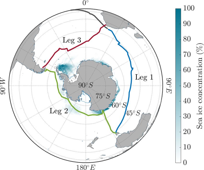
1192                                                          M. H. Derkani et al.: Sea state observations in the Southern Ocean

Figure 2. Examples of sea state conditions: ocean surface during storm conditions (a), sailing through a storm (b), and the marginal ice zone
(c).

Figure 3. Schematic of the wave and surface current monitoring system WaMoS-II (a), example of radar imagery and sub-areas (not in
scale) for post-processing (b), and a sample-derived directional wave energy spectrum (c).

3.2    Measurement principles                                            9 %) were taken during low wind speed and hence removed
                                                                         from the data set.
                                                                            The basic input for extracting sea state features is a se-
The marine radar forms images of the surrounding area based              quence of 64 consecutive images, which correspond to a time
on the backscatter of radar beams. The short wavelets (rip-              period of 175 s (one complete image is acquired for every full
ples) on the ocean surface contribute notably to reflection,             turn of the antenna). Post-processing is carried out on sub-
while long-wave components modulate the returning signal.                areas of 600 m × 1200 m normally taken in front of the ves-
This results in stripe-like patterns in the radar images that            sel, at port and at starboard, to avoid contamination due to the
correspond to the waves (these patterns are known as sea                 ship’s wake (an example of sub-areas is presented in Fig. 3b).
clutters). The system can detect sea clutters reliably only              The temporal sequence for each sub-area, Is (x, y, t), is trans-
if wind speed is greater than 3 m s−1 , which ensures the                formed with a three-dimensional discrete Fourier transform
ocean surface is rough enough (i.e. ripples are developed)               into its spectral domain counterpart; i.e. a three-dimensional
to backscatter the signal efficiently (Hatten et al., 1998). A           image spectrum I (3) (kx , ky , ω), where k = (kx , ky ) is the
small portion of the observations during ACE (approximately              two-dimensional wave number vector, and ω is the angu-

Earth Syst. Sci. Data, 13, 1189–1209, 2021                                                https://doi.org/10.5194/essd-13-1189-2021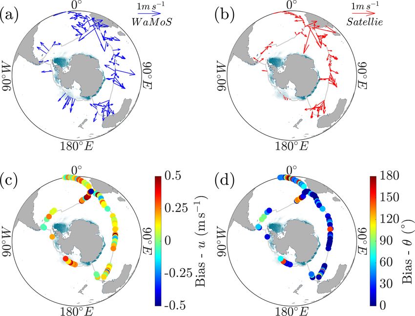
M. H. Derkani et al.: Sea state observations in the Southern Ocean                                                              1193

lar frequency. Assuming linear wave theory (Holthuijsen,             WaMoS-II can detect wavelengths between 15 m and 600 m,
2007), spectral components in I (3) (kx , ky , ω) that correspond    which correspond to wave periods from 3 s to ≈ 16 s.
to ocean waves have to satisfy the linear dispersion relation           Specific wave parameters are derived by integrating
     p                                                               E(f, ϑ). These include the significant wave height, domi-
ω = g|k|tanh(|k|d) + ku,                                       (1)   nant and mean wave periods, associated wavelengths, di-
                                                                     rectional width, and mean wave direction (see Appendix A
where g is the acceleration due to gravity,qd is the water           for a full list of parameters and their definitions). WaMoS-II
depth, u is the surface current, and |k| = kx2 + ky2 is the          also partitions the directional wave energy spectrum to de-
wave number. Spectral components that do not obey Eq. (1)            rive wave heights and periods for wind sea and the first three
are assumed to be noise and hence removed. The remain-               swell systems. The partitioning of the wave spectrum is per-
ing (filtered) three-dimensional image spectrum is integrated        formed using the path-of-steepest-ascent technique (Hanson
over the positive frequency domain to obtain a wave number           and Phillips, 2001), which is a specific implementation of the
image spectrum I (kx , ky ). The latter, however, does not coin-     inverse catchment scheme introduced by Hasselmann et al.
cide with the wave energy spectrum, because it represents the        (1996). The spectral peak that satisfies the condition
intensity of the radar backscatter rather than the amplitude of            U
the water surface elevation (Nieto Borge et al., 1999; Hessner       1.2      cos(θ − ψ) > 1,                                     (3)
                                                                           cp
et al., 2002). Therefore, its zeroth-order moment (m0 ) repre-
sents a signal-to-noise ratio (SNR) instead of the significant       where U is the wind speed, cp is the phase velocity, θ is the
wave height, i.e. a measure of average wave height that is           wave direction, and ψ is the wind direction, is assumed to
                    √
defined as Hs = 4 m0 . Consequently, the image spectrum              be associated with the wind sea. All other systems are swell
requires a re-scaling to convert SNR into the corresponding          and are ranked based on their energy contents as primary,
wave height. This is achieved with the linear regression equa-       secondary, and tertiary swell.
tion (see Nieto Borge et al., 1999, 2004)                               Ocean currents induce a Doppler shift to the wave field.
              √                                                      Both current speed and direction can be quantified by min-
Hs = A + B SNR,                                              (2)     imising the distance between the position of the spectral en-
                                                                     ergy in I (3) (kx , ky , ω) and the theoretical position given by
where A and B are empirical constants that have to be cali-          Eq. (1) using least-squares techniques (Young et al., 1985).
brated following installation. Re-scaling m0 enables correc-         The vessel’s forward speed and heading are used to derive
tion of energy at each spectral mode and derivation of the           the true current.
wave energy spectrum Er (kx , ky ). Radar imaging effects like          Rain, snow, and sea ice produce an excess signal backscat-
tilt modulation, which refers to changes in the effective in-        ter, which results in low-quality images and consequently in-
cidence angle along the long-wave slope, and shadowing,              accurate post-processing products. WaMoS-II automatically
which is caused by the highest waves in the image, con-              assesses the reliability of images through an internal quality
tribute to an inaccurate form of the resulting spectral den-         control protocol (see Hessner et al., 2019), which evaluates
sity function, shifting energy towards high wave numbers             backscatter intensity, number of sea clutters, and stability of
(Nieto Borge et al., 2004). These effects depend on the view         ship motion among other parameters (we remark that tilting
geometry (height and range of the antenna). Consequently,            and shadowing effects are compensated for independently
tilting and shadowing can be assumed to be homogeneous in            using the MTF and do not contribute to quality control). Im-
the relatively small sub-areas used for post-processing and          ages that are deemed of low quality are excluded. The ma-
can be minimised with a single modulational transfer func-           jority of low-quality images were acquired in the marginal
tion (MTF, Nieto Borge et al., 2004). As the imaging effects         ice zone (i.e. south of the 60th parallel) during Leg 2. As a
depend on the wavelength, the MTF is a function of the wave          consequence, observations of waves in ice are not available
number that corrects the spectral density at each mode. An           in the present database.
ensemble average over all sub-areas is computed to derive
the final wave spectrum E(kx , ky ) from the input 64 images.
                                                                     3.3     Underway observations and file types
    In its standard output format, WaMoS-II archives the wave
spectrum as a function of wave frequency, f = ω/2π , and di-         WaMoS-II operated continuously to record observations of
rection, ϑ–E(f, ϑ); the change in variables from wave num-           the sea state during ACE. The vessel was equipped with one
bers to frequency–direction satisfies the dispersion relation in     X-band radar, which was shared between science (requir-
Eq. (1). An example of directional wave spectrum is shown            ing short range settings) and navigational aid (operating at
in Fig. 3c. The resolution of the wave energy spectrum is dic-       medium and long range). Therefore, data acquisition was in-
tated by the size of the sub-areas, which are used to derive the     terrupted anytime the radar was needed for navigation, re-
wave number counterpart in the first instance, and not by the        sulting in gaps in the observations. This was most common
temporal window. Considering the resolution of the image             during Leg 2, as the radar was often switched to long range
(12 m) and the minimum dimension of the sub-area (600 m),            to detect icebergs.

https://doi.org/10.5194/essd-13-1189-2021                                            Earth Syst. Sci. Data, 13, 1189–1209, 2021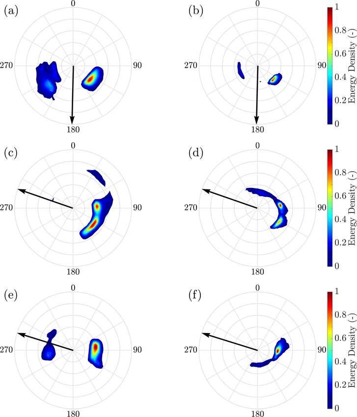
1194                                                    M. H. Derkani et al.: Sea state observations in the Southern Ocean

   The wave spectrum E(f, ϑ) was sampled at 175 s, as-           proach, and, thus, nonlinearities were excluded. The signifi-
suming no gaps or corrupted images occur during the sam-         cant wave height was validated against freely available satel-
pling of 64 consecutive radar images. Output files consist of    lite altimeter data (Ribal and Young, 2019); the scatter plot
(i) the directional wave energy spectrum in the wave num-        of satellite observations versus reconstructed Hs is presented
ber domain (E(kx , ky ), file extension D2S) and frequency–      in Fig. B1 of Appendix B.
directional domain (E(f, ϑ), file extension FTH) and (ii) the        Coefficients A and B in Eq. (2) were estimated using a
(single) one-dimensional frequency–energy spectrum S(f )         maximum likelihood method for the period 9–11 Decem-
obtained by integrating the directional spectrum E(f, ϑ) over    ber 2016 (Leg 0). The root mean square error (RMSE) of the
ϑ (file extension D1S). Each file also includes a header that    fit is 0.21 m, with correlation coefficient R ≈ 0.90 and scatter
provides metadata such as geographical references (latitude      index SI ≈ 0.1. Time series of Hs derived from the IMU sen-
and longitudes), time, wind speed and direction, ship speed      sor and calibrated Hs from WaMoS-II are shown in Fig. 4.
and heading, current speed and direction, and additional in-     Calibrated A and B coefficients were subsequently used to
tegrated parameters.                                             re-scale individual modes of the energy spectrum.
   WaMoS-II also performed a running average over 20 min
to minimise the effects of natural variability. Output files
                                                                 4     Overview of sea state conditions
consist of (i) the mean directional wave energy spectrum in
both wave number and frequency–directional domain (file          4.1    Sea state climate during ACE
extensions D2M and FTM, respectively) and (ii) the mean
one-dimensional frequency–energy spectrum (file extension        Excluding the regions south of the 60th parallel, which un-
D1M). These files are sampled every 175 s, with the first one    dergo a strong seasonal sea ice cycle (Eayrs et al., 2019), the
20 min after starting the equipment.                             Southern Ocean is normally characterised by weak seasonal
   In addition, time series of wind, current, and wave vari-     variability (Young et al., 2020). Therefore, extreme sea states
ables from mean directional wave spectra are archived in         remain likely even during summer. As a reference, wind, cur-
monthly summary files.                                           rent, and wave climate statistics in the form of the 50th and
                                                                 90th percentiles (hereafter P50 and P90, respectively) aggre-
3.4    Calibration
                                                                 gated in 2◦ × 2◦ regions for the summer months (December,
                                                                 January, February) are reported in Fig. 5. Data of wind speed
The calibration of coefficients A and B in Eq. (2) was per-      and wave height are from all satellite missions mounting al-
formed by forcing the SNR to match independent benchmark         timeter sensors that are available from 1985 to 2019 (Ribal
observations of Hs . The reference values were reconstructed     and Young, 2019). Data of current speed are from the Coper-
from records of ship motion, which were measured through-        nicus GlobCurrent database – https://marine.copernicus.eu
out the expedition with an inertial measurement unit (IMU)       (last access: 8 July 2020) – that combines the velocity field of
at a sampling rate of 1 Hz (Alberello et al., 2020b; Landwehr    geostrophic surface currents from satellite sensors recorded
et al., 2021).                                                   from 1993 to 2019 (Rio et al., 2014) and modelled Ekman
   An overview of ship motion to sea state conversion (the       currents, which include components from wind stress forc-
wave buoy analogy) can be found in for example Nielsen           ing obtained from atmospheric system and drifter data.
(2017). The method relies on the principle that the vessel is       The wind speed is represented by its value at 10 m above
a rigid body with six degrees of freedom (three translations:    sea level (U10 ). Apart from a region east of Argentina, where
heave, surge, and sway; and three rotations: pitch, roll, and    the South American continent induces a shadowing effect,
yaw) that moves in response to the incident   R wave field ex-   wind speed is fairly uniform throughout the ocean: P50 varies
pressed as the frequency spectrum S(f ) = E(f, ϑ) dϑ and         between 10 and 12 m s−1 , while P90 ranges between 15 and
restoring forces expressed as a function of its mass, geome-     18 m s−1 (see Fig. 5a and b). Close to the Antarctic conti-
try, loading conditions, and forward speed, among other pa-      nent and outside the belt of the strong westerly winds (south
rameters (Newman, 2018). The relation between the ship mo-       of the 70th parallel), wind speed weakens with P50 reducing
tion and the wave field is evaluated via the response ampli-     to ≈ 3 m s−1 and P90 to ≈ 10 m s−1 . There are also low wind
tude operator (R(f ); see Newman, 2018), i.e. a ship-specific    speeds (U10 < 3 m s−1 for both P50 and P90) in the lee of the
function that translates the motion spectrum Sship (f ) into     Antarctic Peninsula, although this may relate to uncertainties
the wave spectrum: S(f ) = Sship (f )/R(f )2 . Motion spectra    due to a high concentration of sea ice (see Fig. 1) and/or the
were evaluated by applying a discrete Fourier transform to       increased drag over sea ice compared to open water (Mar-
5 min long time series of heave motion. An approximation of      tinson and Wamser, 1990). Note that, excluding the station
R(f ) for the Akademik Tryoshnikov was calculated solving        at Mount Siple, the expedition remained within the belt of
the equation of motion with a model based on the boundary        westerly winds.
element method (NEMOH, Babarit and Delhommeau, 2015)                Significant wave height Hs follows the wind pattern, un-
and taking into account the ship’s heading, forward speed,       derpinning the dominance of wind seas on swell systems.
and loading conditions. The model is based on a linear ap-       Between 40◦ and 60◦ S, the belt where most of Leg 1 and

Earth Syst. Sci. Data, 13, 1189–1209, 2021                                       https://doi.org/10.5194/essd-13-1189-2021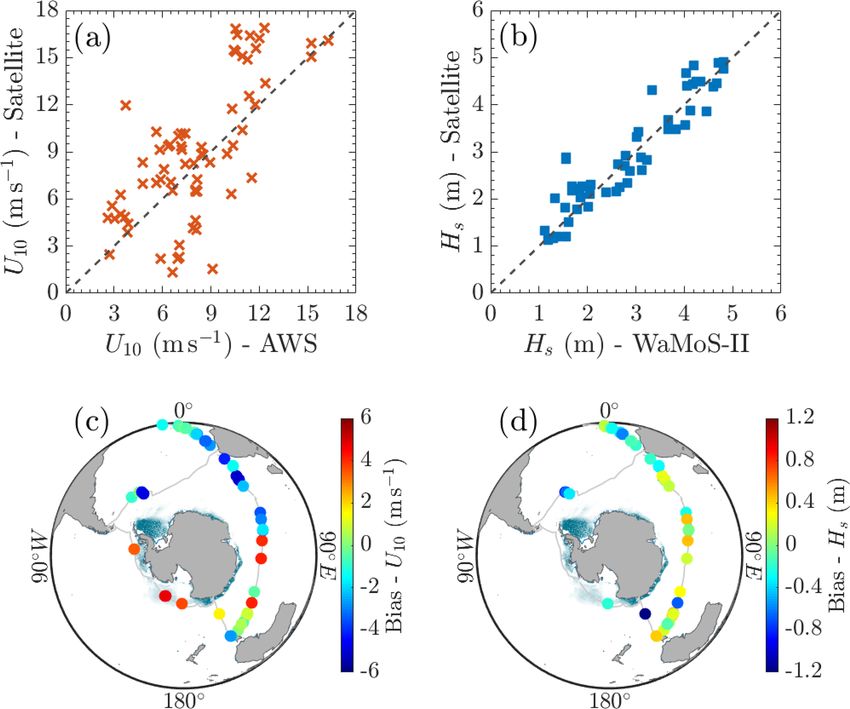
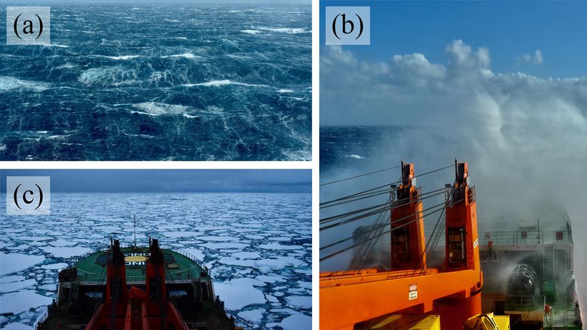
M. H. Derkani et al.: Sea state observations in the Southern Ocean                                                                      1195

Figure 4. Time series of significant wave height Hs : benchmark observations derived from ship motion data (red dots) and calibrated records
from WaMoS-II (blue solid line).

Figure 5. Wind speed (U10 ), significant wave height (Hs ), and surface current speed (u) climatology in Austral summer: (a) 50th percentile
(median) wind speed, (b) 90th percentile wind speed, (c) 50th percentile (median) significant wave height, (d) 90th percentile significant
wave height, (e) 50th percentile (median) surface current speed, and (f) 90th percentile surface current speed. Latitudes are shown every 15◦
(from 15 to 90◦ S) by thin lines; the route of the ACE voyage is reported as a black solid line; and the sea ice edge, defined by the 10 % sea
ice concentration, is shown as a grey solid line.

https://doi.org/10.5194/essd-13-1189-2021                                                 Earth Syst. Sci. Data, 13, 1189–1209, 2021
1196                                                       M. H. Derkani et al.: Sea state observations in the Southern Ocean

Leg 3 took place, P50 ≈ 3.5 m, and P90 ranges between 5             largest waves (Hs > 6 m) were encountered at the beginning
and 6 m (Fig. 5c and d). There is an evident shadowing ef-          of Leg 2 (see photos of the sea state in Fig. 2a and b). There-
fect east of the Drake Passage, due to a combination of lower       after, Hs was less than 2 m as a result of the interaction with
wind speed and a reduction of fetches. South of the 60th par-       sea ice (see Fig. 2c). The crossing of the Drake Passage at
allel (Leg 2), Hs drops notably with the P50 decreasing to          the end of Leg 2 did not record significantly large waves, with
≈ 2 m and P90 reducing to ≈ 4 m, despite strong westerly            Hs ≈ 4 m at most. Wave periods were generally long and nor-
winds being active down to 70◦ S. The attenuation is induced        mally in excess of 8 s (> 100 m wavelengths), substantiating
by sea ice (Bennetts et al., 2015; Toffoli et al., 2015; Mon-       the extensive (almost infinite) fetches for wave development.
tiel et al., 2016), which has high concentration close to the       Concomitantly with almost all storms, Tm−10 increased and
Antarctic coastline, even in the summer months, especially          reached maximum values of 11–12 s (wavelengths ≈ 200 m).
in the western Pacific, Ross Sea and Amundsen Sea sectors              The majority of Leg 1 and Leg 3 followed the Antarctic
of Antarctica (see Fig. 1).                                         Circumpolar Current with records of surface current speeds
   The speed of the Antarctic Circumpolar Current has P50           oscillating around 0.5 m s−1 . Interestingly, observations were
≈ 0.5 m s−1 . The P90 shows velocity with maxima in excess          notably higher than P90 for the majority of the expedition.
of 0.75 m s−1 , especially in the Indian Ocean sector (first half   Despite being primarily south of the polar front, currents
of Leg 1). Besides the Antarctic Circumpolar Current, ACE           faster than P90 were also recorded in Leg 2, primarily in the
crossed two regions with strong currents: the Agulhas region,       marginal ice zone. ACE crossed two regions characterised by
where P90 excess 1.5 m s−1 ; and the Argentine basin (begin-        strong surface currents: east of South Africa at the southern-
ning of Leg 3), where a northward extension of the Antarctic        most edge of the Agulhas Current (beginning of Leg 1), with
Circumpolar Current forces water flow to speeds of approxi-         speeds up to 2 m s−1 ; and east of South America where the
mately 1 m s−1 . South of the polar front (latitudes higher than    Antarctic Circumpolar Current has a northward extension,
60◦ S), there is no significant circulation pattern, with maxi-     with surface speeds recorded up to 1.8 m s−1 . Observations at
mum current speed less than 0.3 m s−1 (see Fig. 5f).                both locations exceeded P90 notably. We remark that P50 and
                                                                    P90 include the contribution of geostrophic surface currents
4.2    Observed sea states during ACE
                                                                    and wind stresses. However, additional components such as
                                                                    inertial oscillations (Treguier and Klein, 1994) are not taken
Figure 6 shows time series for the entire expedition of 10 m        into account due to the coarse resolution of satellite observa-
true wind speed (U10 ), significant wave height (Hs ), and cur-     tions and Ekman components. To some extent, the absence of
rent speed (u). As a benchmark, collocated values of P50,           inertial oscillations in climate statistics substantiates the sig-
their interquartile range (IQR), and P90 are reported in the        nificant current speeds recorded by the WaMoS-II. Further,
figure. Time series of mean wave period (Tm−10 ), wave direc-       Ekman components remain uncertain in the Southern Ocean
tional spreading (σθ ), inverse wave age (µ), and wave steep-       due to inaccuracies in estimating wind stress from the atmo-
ness (ε) are presented in Fig. 7. Definitions of the variables      spheric system, adding inconsistencies to benchmark statis-
are reported in Appendix A.                                         tics.
   Overall, the observed median wind speed was 7.25 m s−1 ,            An intrinsic feature of oceanic sea states is the direc-
with an interquartile (IQ) of 5.1 m s−1 . During Leg 1, the ex-     tional distribution of the spectral density function (Mitsuyasu
pedition went through six storm events with wind speeds re-         et al., 1975; Donelan et al., 1985; Young and Verhagen, 1996;
ported in excess of 12 m s−1 (P50 ≈ 10 m s−1 ). Two of these        Toffoli et al., 2017; Fadaeiazar et al., 2020; Young et al.,
events were equal to or greater than the P90 for the season         2020), which is summarised in the form of a mean direc-
(≈ 15 m s−1 ). Leg 2 started with the most extreme storm dur-       tional spreading (i.e. the circular standard deviation of the
ing ACE; winds reached speeds close to 20 m s−1 , which is          directional wave energy spectrum). Sea states dominated by
well above P90. The remainder of Leg 2 was characterised by         strong winds are normally characterised by a broad spreading
relatively low wind speeds, consistent with P50. Two more           with σϑ > 40◦ (Donelan et al., 1985). These conditions were
storms with wind speeds in excess of P90 were encoun-               reported consistently throughout the expedition, with maxi-
tered at the end of Leg 2, while approaching and crossing           mum mean directional spreading reaching values as large as
the Drake Passage. The final leg was also characterised by          80◦ . Narrow directional distributions (σϑ ≤ 30◦ ) were also
intense storms with wind speeds notably above P50 for al-           common and primarily recorded in between storms, where
most the entire leg. Three significant storm events with wind       the sea state was dominated by swells.
speeds above P90 (U10 ≈ 18 m s−1 ) were reported.                      The inverse wave age µ and the wave steepness ε are pa-
   The median significant wave height during the expedi-            rameters that estimate the stage of growth of the wave field.
tion was 2.61 m and IQ ≈ 1.6 m. To avoid the most ener-             Both variables are associated with nonlinear mechanisms
getic waves, the ship’s course was continuously adapted to          that lead to large (extreme) waves (Onorato et al., 2009; Tof-
bypass storms. Despite this, intense wave conditions were           foli et al., 2017), wave breaking (Toffoli et al., 2010), and,
encountered, with Hs reaching the P90 (≈ 5 m) during al-            thus, ocean–atmosphere fluxes (Schmale et al., 2019; Thurn-
most all storm events, especially during Leg 1 and Leg 3. The       herr et al., 2020). The inverse wave age is the ratio of wind

Earth Syst. Sci. Data, 13, 1189–1209, 2021                                           https://doi.org/10.5194/essd-13-1189-2021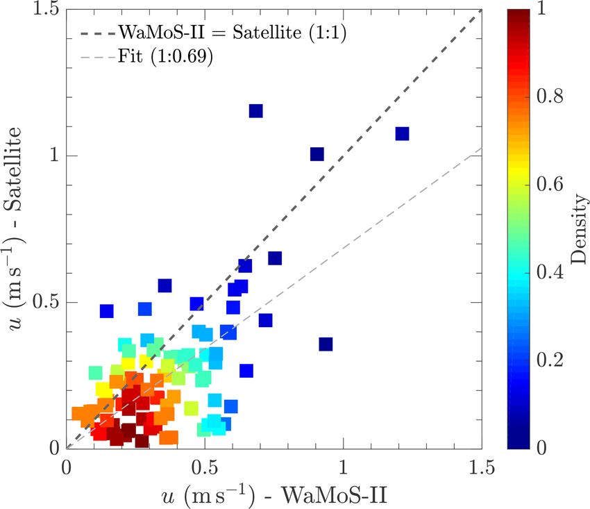
M. H. Derkani et al.: Sea state observations in the Southern Ocean                                                                        1197

Figure 6. Time series of sea state variables in Leg 1 (blue), Leg 2 (green), and Leg 3 (red): (a) wind speed from the automated weather
station, (b) significant wave height, and (c) current speed. For each variable, the dashed line and shading represent the 50th percentile and its
interquartile range IQR, respectively, based on climate statistics from satellite observations; the solid line indicates the 90th percentile.

Figure 7. Time series of sea state variables in Leg 1 (blue), Leg 2 (green), and Leg 3 (red): (a) mean wave period, (b) mean directional
spread, (c) inverse wave age, and (d) wave steepness. Details of variables are reported in Appendix A.

https://doi.org/10.5194/essd-13-1189-2021                                                   Earth Syst. Sci. Data, 13, 1189–1209, 2021
1198 M. H. Derkani et al.: Sea state observations in the Southern Ocean
Figure 8. Wind from the automated weather station and significant wave height from WaMoS-II versus satellite observations: scatter dia-
grams (a, b) and geographical distribution of biases (c, d). Average sea ice concentration during the expedition is overlaid in panels (c) and
(d).
speed to wave phase velocity (i.e. the ratio of wavelength 1Y = 0.5◦ and temporal resolution of 1t = 3 h. Although
to period). Following their generation, waves grow in height satellite observations have been quality controlled and cali-
and length until they move faster than winds (Holthuijsen, brated against available in situ sensors (see details in Ribal
2007). For µ > 0.8, waves are “young” as they are in a grow- and Young, 2019), the scarcity of in situ data in the Southern
ing phase. This condition is normally characterised by a steep Ocean leaves uncertainties in the data set.
profile, which leads to breaking. Young waves were recorded Figure 8 shows scatter diagrams of matching averages at
during all storm events with steepness generally in excess of collocated clusters (panels a and b) and geographical distri-
0.1. For µ < 0.8, the waves no longer receive energy from butions of biases (difference between WaMoS-II and satellite
wind as they have reached full development. The shape of observations, panels c and d). Overall, in situ measurements
waves is gently sloping (i.e. the wave steepness is small) and of wind speeds during ACE are consistent with concurrent
breaking is unlikely (the ocean is dominated by swell). Dur- satellite observations, with data lying along the 1 : 1 correla-
ing the most extreme events at the beginning of Leg 2, steep- tion line. Nevertheless, there is a notable RMSE ≈ 3.2 m s−1 ,
ness reached a maximum of about 0.13. This is an excep- with R ≈ 0.70 and SI ≈ 0.360. Biases show both overestima-
tionally high value for ocean waves and is normally associ- tions (especially at the beginning of Leg 1 and Leg 3) and
ated with the formation of rogue waves (Onorato et al., 2009; underestimation (at the end of Leg 1 and Leg 2) of satel-
Toffoli et al., 2010). lite observations, varying between −6 and 6 m s−1 . The most
substantial positive biases are reported in the marginal ice
5 Comparison against satellite observations zone, where Antarctic sea ice affects wind speed detection.
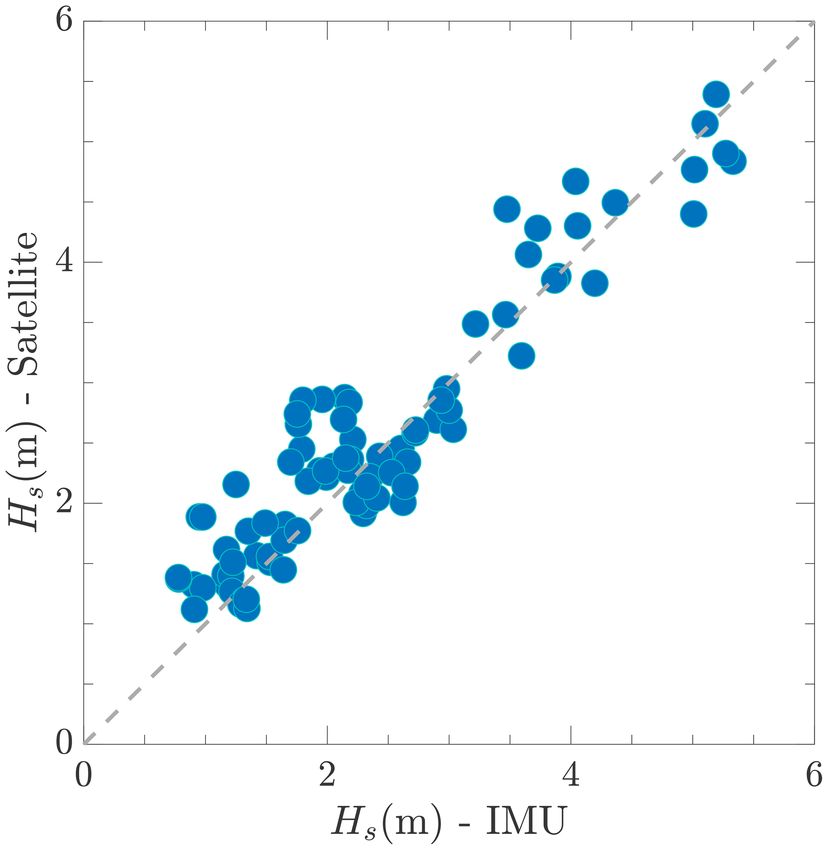
Significant wave heights match better with satellite obser-
5.1 Wind speed and significant wave height vations than wind speeds, with RMSE ≈ 0.42 m, R ≈ 0.93,
and SI ≈ 0.155. Most of the collocated observations were
Wind speeds and significant wave heights are compared found in Leg 1. Overall, the bias is positive, indicating a
against collocated satellite observations from altimeter sen- slight underestimation of the sea state from satellite sen-
sors (same data source discussed in the previous session). sors. The largest biases (ranging between 0.4 and 1.2 m) were
Due to the scattered nature of satellite data, average values
are computed for clusters with spatial resolution of 1X =
Earth Syst. Sci. Data, 13, 1189–1209, 2021 https://doi.org/10.5194/essd-13-1189-2021M. H. Derkani et al.: Sea state observations in the Southern Ocean 1199 Figure 9. Example directional wave energy spectra recorded during ACE (a, c, e) and collocated SAR spectra (b, d, f). Wind direction recorded during ACE is shown as black arrows. Both the wave spectra and wind direction follow the “coming from” convention. Circles in the polar plot indicate frequencies from 0.05 Hz (innermost) to 0.25 Hz (outermost) with a step of 0.05 Hz; radiant lines indicate direction with a 30◦ step. Figure 10. Comparison of integrated parameters (WaMoS-II versus SAR): significant wave height (Hs , panel a), energy wave period (Tm−10 , panel b), and wave directional spreading (σθ , panel c). https://doi.org/10.5194/essd-13-1189-2021 Earth Syst. Sci. Data, 13, 1189–1209, 2021
1200                                                     M. H. Derkani et al.: Sea state observations in the Southern Ocean

linked to storm events and are ≈ 10 % of the in situ-measured
values.

5.2    Directional wave spectrum

Altimeter sensors only measure specific variables, namely
the significant wave height and the wind speed, whereas SAR
imagery can be converted into a directional wave energy
spectrum (e.g. Collard et al., 2009). Collocated SAR spectra
from Sentinel-1A/1B missions within area of 0.5◦ ×0.5◦ and
maximum temporal difference of 6 h were retrieved from the
Australian Ocean Data Network (AODN) portal (Khan et al.,
2020b). Overall, 10 SAR spectra were found during ACE,
with ≈ 70 % of them in the Indian Ocean during Leg 1.
   Examples of collocated wave spectra from WaMoS-II and
SAR are presented in Fig. 9; mean wind direction is also re-
ported. We remark that SAR detects wavelength longer than
115 m (approximately, wave periods exceeding 8 s or fre-
quencies below 0.1 Hz) and represented swell systems pri-         Figure 11. Scatter plot of WaMoS-II surface current speeds against
marily. WaMoS-II, on the contrary, captures the full spec-        observations derived from satellite sensors.
trum, including the short wavelengths of the wind sea. Within
the operational range of SAR (f < 0.1 Hz in the figure), the
spectral shape from both sensors agrees well, especially for      30 % larger than the latter. Other basic metrics of the scatter
the portion around the primary (most energetic) swell. No-        diagram are RMSE ≈ 0.2 m s−1 , R ≈ 0.63, and SI ≈ 0.80.
table discrepancies, however, are evident for less energetic      Biases associated with current speed are uniformly dis-
secondary peaks, for which the relative uncertainty grows.        tributed across the expedition. A relatively small bias was
High-frequency components (f > 0.1 Hz) are not resolved in        detected in Leg 1, when sailing along the Antarctic Circum-
SAR but appear in the WaMoS-II spectra. Note that the mis-        polar Current. The largest biases (about 0.5 m s−1 , the same
alignment of high-frequency components with the wind di-          order of magnitude of the current speed itself) were detected
rection in the upper two panels is due to recent wind change.     primarily at the beginning of Leg 1 and at the end of Leg 3,
   To provide a more robust comparison, scatter diagrams          where the ship crossed the Agulhas Current, and in Leg 2,
for Hs , Tm−10 , and σϑ are presented in Fig. 10. For con-        when crossing the Antarctic marginal ice zone. The reported
sistency, wave spectra from WaMoS-II have been filtered           differences are linked to inconsistencies between WaMoS-
to eliminate high-frequency modes that are not detected           II and benchmark data due to inertial oscillations (Treguier
by SAR (f > 0.117 Hz or wavelength L < 115 m). SAR and            and Klein, 1994), which are not detected by satellite obser-
WaMoS-II observations agree well, with RMSE ≈ 0.36 m,             vations, and inaccuracy of wind stresses in the Ekman com-
R ≈ 0.92, and SI ≈ 0.20 for Hs ; RMSE ≈ 0.42 s, R ≈ 0.92,         ponents.
and SI ≈ 0.038 for Tm−10 , noting wave periods from SAR              Current direction is generally in better agreement with
are consistently (slightly) higher than WaMoS-II’s; and           satellite observations than speed (see Fig. 12a and b). Dif-
RMSE ≈ 13.41◦ , R ≈ 0.56, and SI ≈ 0.295 for σϑ , despite         ferences between WaMoS-II altimeter sensors are normally
two outliers.                                                     small throughout the expedition, with common values of
                                                                  about 10◦ . The only substantial differences were recorded at
                                                                  the beginning of Leg 3, east of South America.
5.3    Surface current

Figure 11 shows the scatter diagram comparing surface cur-        6   Data availability
rent speeds from WaMoS-II and collocated observations de-
rived from altimeter sensors (Rio et al., 2014). The geograph-    Data are available through the Australian Antarctic Data
ical distributions of current speeds, directions, and concur-     Centre: (i) Alberello et al. (2020c) contains data sets of wave
rent differences between WaMoS-II and altimeter sensors are       spectra including files D1S, D2S, D1M, D2M, and FTH
presented in Fig. 12. Note that values in both figures repre-     (https://doi.org/10.26179/5ed0a30aaf764); and (ii) Derkani
sent averages of observations falling in clusters of 0.5◦ ×0.5◦   et al. (2020) contains time series of wind speed and di-
with temporal resolution of 0.5 h.                                rection, current speed and direction, sea state parameters
   Contrary to wind and wave parameters, current speeds           including wave height, period, wavelength and mean di-
from WaMoS-II show notable differences from satellite ob-         rection for total sea, wind sea and swell systems, ship
servations. The former produces current speeds that are about     course, position, and speed for each month of the expedition

Earth Syst. Sci. Data, 13, 1189–1209, 2021                                         https://doi.org/10.5194/essd-13-1189-2021
M. H. Derkani et al.: Sea state observations in the Southern Ocean 1201
Figure 12. Surface current velocities along the ACE voyage: WaMoS-II (a) and space-borne altimeter sensors (b). Surface current biases
between WaMoS-II and satellite observations for current speed (c) and direction (d). Average sea ice concentration during the expedition is
overlaid in all panels.
(https://doi.org/10.26179/5e9d038c396f2). Day and time of from satellite-borne sensors to verify the robustness of the
available measurements can be found in the file Avail- database.
able_Measurements_List.txt, which is included in Alberello The data set includes observations around the Southern
et al. (2020c). Ocean from latitude 34 to 74◦ south. This comprises records
in the open ocean across the Antarctic Circumpolar Current
and in the Antarctic marginal ice zone. Due to its exposure
to strong westerly winds, the Southern Ocean is subjected to
7 Conclusions
harsh sea state conditions all year round. Although the ex-
pedition took place during the Austral summer, the data set
The scarcity of field observations in the Southern Ocean contains records of severe sea states, in excess of the 90th
hampers the accuracy of satellite sensors and prediction mod- percentile expected for the season.
els. In response to this issue, a unique data set of sea state The expedition was conceived to bring together a broad
parameters, comprising concomitant observations of winds, range of Earth Science disciplines with the aim of exploring
waves, and surface currents, was recorded in the Southern the interplay of processes in the lower atmosphere, ocean sur-
Ocean during the Antarctic Circumnavigation Expedition, face, subsurface, and land with simultaneous observations.
from December 2016 to March 2017. Measurements were Additional data sets of atmospheric and oceanic variables
obtained using a radar-based wave and surface current mon- that relate to sea state can be found in Schmale et al. (2019),
itoring system (WaMoS-II) and complemented with records Rodríguez-Ros et al. (2020), Smart et al. (2020), Thurnherr
of winds from the meteorological station on board the re- et al. (2020), and Suaria et al. (2020). These include, but are
search icebreaker Akademik Tryoshnikov. Despite some gaps, not limited to, air–sea fluxes (mass, gas, heat, and momen-
observations of wind speeds and directions; directional wave tum), aerosol concentrations, stable water isotopologues, and
energy spectra; integrated parameters such as wave heights, micro-fibres. Collocated observations have been the foun-
mean wave periods, and wavelengths; and current speeds dation for research on moist diabatic processes (Thurnherr
and directions were collected underway during the entire et al., 2020) and sea spray aerosols dynamics (Landwehr
expedition with outputs every 175 s. The sea state monitor- et al., 2021), demonstrating capacities for surface waves
ing system was calibrated with benchmark sea state records, to modulate water isotopologue concentrations and marine
which were reconstructed from the ship motion. Measure- aerosols emissions, settling velocity and lifetime in the ma-
ments were also compared against available observations
https://doi.org/10.5194/essd-13-1189-2021 Earth Syst. Sci. Data, 13, 1189–1209, 20211202 M. H. Derkani et al.: Sea state observations in the Southern Ocean rine boundary layer up to the cloud condensation height. The presented database has further potentials to support research enhancing wave model performances in the Southern Ocean, wave dynamics, including occurrence of rogue waves, wave dissipation mechanisms as well as other coupled processes, including those interconnecting waves with the upper ocean and sea ice in the Antarctic marginal ice zone. Earth Syst. Sci. Data, 13, 1189–1209, 2021 https://doi.org/10.5194/essd-13-1189-2021
M. H. Derkani et al.: Sea state observations in the Southern Ocean                                        1203

Appendix A: WaMoS-II sea state parameters

Details of sea-state-related variables from WaMoS-II out-
put files as well as integrated parameters are described in
Table A1. The nth-order moment of the spectral density
function,
R R n mn , referred to in the table is defined as mn =
    f E(f, ϑ) df dϑ. Directional Fourier coefficients a and
b used to compute the wave directional spreading are as fol-
lows:
    Z Z
a=        cos(ϑ)S(f, ϑ)df dϑ,                          (A1)
    Z Z
b=        sin(ϑ)S(f, ϑ) df dϑ.                         (A2)

https://doi.org/10.5194/essd-13-1189-2021                            Earth Syst. Sci. Data, 13, 1189–1209, 2021
1204 M. H. Derkani et al.: Sea state observations in the Southern Ocean
Table A1. WaMoS-II output and integrated sea-state-related parameters and their symbol, definition, range, and accuracy. “n/a” stands for
“not applicable”.
Sea-state-related parameter Symbol Definition Range Accuracy
10 m true wind speed and direction (m s−1 , ◦ ) U10 , α – – –
Two-dimensional wave number spectrum (m4 ) E(kx , ky ) Refer to Sect. 3.2 – n/a
Two-dimensional frequency–direction spec- E(f, ϑ) |k| ∂|k|
∂ω E(kx , ky ) 0.0078–0.5000 Hz, 0–360◦ n/a
trum (m2 (Hz × rad)−1 )
R 360◦
One-dimensional S(f ) 0 E(f, ϑ)dϑ 0.0078–0.5000 Hz n/a
frequency spectrum (m2 Hz−1 )
Significant wave height (m) HS Refer to Eq. (2) 1–20 m ±0.5 m
m
Energy wave period (s) Tm−10 Tm−10 = m−1
0
3.5–55 s ±0.5 s
Peak wave period (s) Tp 1 3.5–55 s ±0.5 s
fp
Mean wave direction (◦ ) βm arctan(b/a) 0–360◦ ±2◦
Peak wave direction (◦ ) βp ϑ(fp ); fp = T1 0–360◦ ±2◦
p
gT 2 r
2
Peak wave length (m) λp λp = 2πp tanh( 4π2 dg ) 19–600 m –
Tp
√
First, second, and third significant wave height Hs1,2,or3 4 m01,2,or3 1–20 m ±0.5 m
for swell systems 1, 2, and 3 (m)
First, second, and third wave peak period for Tp1,2,or3 1 3.5–55 s ±0.5 s
fp1,2,or3
swell systems 1, 2, and 3 (s)
First, second, and third wave length for swell λ1,2,or3 2π 19–600 m –
|k p1,2,or3 |
systems 1, 2, and 3 (m)
First, second, and third wave direction for swell β1,2,or3 ϑ(fp1,2,or3 ) 0–360◦ ±2◦
systems 1, 2, and 3 (◦ )
s
180
r
a 2 +b2 ]
√ ◦
Wave directional spreading (◦ ) σθ π 2[1 − 0 − 180
π 2 n/a
m20
U10
Inverse wave age (−) µ cp , cp : wave phase velocity – –
Wave steepness (−) ε k H2S – –
Surface current speed (m s−1 ) u Refer to Eq. (1) 0–20 m s−1 ±0.2 m s−1
Surface current direction (◦ ) θ Refer to Eq. (1) 0–360◦ ±2◦
Earth Syst. Sci. Data, 13, 1189–1209, 2021 https://doi.org/10.5194/essd-13-1189-2021M. H. Derkani et al.: Sea state observations in the Southern Ocean 1205 Appendix B: Validation of ship motion to sea state conversion Significant wave heights reconstructed from ship motion data were validated against freely available satellite obser- vations (Ribal and Young, 2019) for the entire ACE voy- age (see scatter plot in Fig. B1). Due to the coarse resolu- tion of satellite data, average values are computed for clus- ters with spatial resolution of 0.5◦ × 0.5◦ and temporal res- olution of 3 h. Overall, there is a good agreement between reconstructed and observed sea state. The root-mean squared error (RMSE) is 0.4 m, the correlation coefficient (R) is 0.94, and the scatter index (SI) is 0.17. Similar error metrics are obtained by comparing the reconstructed sea state against parameters from the European Centre for Medium-Range Weather Forecasts (ECMWF – https://www.ecmwf.int/en/ forecasts/datasets/reanalysis-datasets/era5, last access: 7 De- cember 2020) ERA-5 database. Figure B1. Satellite observations versus significant wave height re- constructed from ship motion. https://doi.org/10.5194/essd-13-1189-2021 Earth Syst. Sci. Data, 13, 1189–1209, 2021
1206                                                            M. H. Derkani et al.: Sea state observations in the Southern Ocean

Author contributions. KR, KMH, and AT participated to the ex-              WaMoS Data, Ver. 3, Australian Antarctic Data Centre,
pedition and acquired the data. MHD, AA, LGB, and AT conceived             https://doi.org/10.26179/5ed0a30aaf764, 2020c.
the manuscript. KGH provided on-shore technical support and LA           Aouf, L., Hauser, D., Chapron, B., Toffoli, A., Tourrain, C.,
provided marine forecast during the expedition. MHD and KGH                and Peureux, C.: New directional wave satellite observations:
calibrated and analysed the data. FN provided benchmark obser-             Towards improved wave forecasts and climate description in
vation for calibration. LA and SK provided SAR spectra. All au-            Southern Ocean, Geophys. Res. Lett., 48, e2020GL091187,
thors contributed to the data interpretation and to the writing of the     https://doi.org/10.1029/2020GL091187, 2020.
manuscript.                                                              Babanin, A. V.: On a wave-induced turbulence and a wave-
                                                                           mixed upper ocean layer, Geophys. Res. Lett., 33, L20605,
                                                                           https://doi.org/10.1029/2006GL027308, 2006.
Competing interests. The authors declare that they have no con-          Barbariol, F., Benetazzo, A., Bertotti, L., Cavaleri, L., Durrant, T.,
flict of interest.                                                         McComb, P., and Sclavo, M.: Large waves and drifting buoys in
                                                                           the Southern Ocean, Ocean Eng., 172, 817–828, 2019.
                                                                         Babarit, A. and Delhommeau, G.: Theoretical and numerical as-
Acknowledgements. This work was part of the Antarctic Cir-                 pects of the open source BEM solver NEMOH, in: Proc.
cumnavigation Expedition (ACE). MHD was partially supported by             of the 11th European Wave and Tidal Energy Conference
a PhD top-up scholarship from the Australian Bureau of Meteorol-           (EWTEC2015), September 2015, Nantes, France, ID: hal-
ogy. MHD, AA, FN and AT acknowledge technical support form                 01198800, 2015.
the Air-Sea-Ice Lab initiative.                                          Bennetts, L. G., Alberello, A., Meylan, M. H., Cavaliere, C., Ba-
                                                                           banin, A. V., and Toffoli, A.: An idealised experimental model of
                                                                           ocean surface wave transmission by an ice floe, Ocean Model.,
                                                                           96, 85–92, https://doi.org/10.1016/j.ocemod.2015.03.001, 2015.
Financial support. This research has been supported by the ACE
                                                                         Bennetts, L. G., O’Farrell, S., and Uotila, P.: Brief commu-
Foundation and Ferring Pharmaceuticals (Project 17), the CRC-P
                                                                           nication: Impacts of ocean-wave-induced breakup of Antarc-
initiative of the Australian Government (grant no. CRC- P53991),
                                                                           tic sea ice via thermodynamics in a stand-alone version of
and the Australian Antarctic Program (grant no. AAS 4434).
                                                                           the CICE sea-ice model, The Cryosphere, 11, 1035–1040,
                                                                           https://doi.org/10.5194/tc-11-1035-2017, 2017.
                                                                         Collard, F., Ardhuin, F., and Chapron, B.: Monitoring and
Review statement. This paper was edited by Giuseppe M.R.                   analysis of ocean swell fields from space: New methods
Manzella and reviewed by three anonymous referees.                         for routine observations, J. Geophys. Res., 114, C07023,
                                                                           https://doi.org/10.1029/2008JC005215, 2009.
                                                                         Csanady, G. T.: Air-sea interaction: laws and mechanisms, Cam-
                                                                           bridge University Press, Cambridge, 2001.
References                                                               Derkani, M., Alberello, A., and Toffoli, A.: Antarctic Circumnavi-
                                                                           gation Expedition 2017: WaMoS Data Product, Ver. 1, Australian
Ackley, S. F., Stammerjohn, S., Maksym, T., Smith, M., Cassano,            Antarctic Data Centre, https://doi.org/10.26179/5e9d038c396f2,
  J., Guest, P., Tison, J. L., Delille, B., Loose, B., Sedwick, P.,        2020.
  DePace, L., Roach, L., and Parno, J.: Sea-ice production and           Donelan, M. A., Hamilton, J., and Hui, W. H.: Directional spectra of
  air/ice/ocean/biogeochemistry interactions in the Ross Sea dur-          wind-generated ocean waves, Philos. T. R. Soc. A, 315, 509–562,
  ing the PIPERS 2017 autumn field campaign, Ann. Glaciology,              1985.
  61, 181–195, https://doi.org/10.1017/aog.2020.31, 2020.                Dong, S., Gille, S. T., and Sprintall, J.: An assessment of the South-
Alberello, A., Onorato, M., Bennetts, L., Vichi, M., Eayrs, C.,            ern Ocean mixed layer heat budget, J. Climate, 20, 4425–4442,
  MacHutchon, K., and Toffoli, A.: Brief communication: Pan-               2007.
  cake ice floe size distribution during the winter expansion of         Dong, S., Sprintall, J., Gille, S. T., and Talley, L.: Southern Ocean
  the Antarctic marginal ice zone, The Cryosphere, 13, 41–48,              mixed-layer depth from Argo float profiles, J. Geophys. Res.,
  https://doi.org/10.5194/tc-13-41-2019, 2019a.                            113, C06013, https://doi.org/10.1029/2006JC004051, 2008.
Alberello, A., Onorato, M., Frascoli, F., and Toffoli, A.: Observa-      Eayrs, C., Holland, D., Francis, D., Wagner, T., Kumar, R., and Li,
  tion of turbulence and intermittency in wave-induced oscillatory         X.: Understanding the Seasonal Cycle of Antarctic Sea Ice Ex-
  flows, Wave Motion, 84, 81–89, 2019b.                                    tent in the Context of Longer-Term Variability, Rev. Geophys.,
Alberello, A., Bennetts, L., Heil, P., Eayrs, C., Vichi, M.,               1037–1064, https://doi.org/10.1029/2018RG000631, 2019.
  MacHutchon, K., Onorato, M., and Toffoli, A.: Drift of Pan-            Fadaeiazar, E., Leontini, J., Onorato, M., Waseda, T., Alberello, A.,
  cake Ice Floes in the Winter Antarctic Marginal Ice Zone During          and Toffoli, A.: Fourier amplitude distribution and intermittency
  Polar Cyclones, J. Geophys. Res.-Oceans, 125, e2019JC015418,             in mechanically generated surface gravity waves, Phys. Rev.
  https://doi.org/10.1029/2019JC015418, 2020a.                             E, 102, 013106, https://doi.org/10.1103/PhysRevE.102.013106,
Alberello, A., Bennetts, L., and Toffoli, A.: Antarc-                      2020.
  tic Circumnavigation Expedition 2017: Motion Sen-                      Hanson, J. L. and Phillips, O. M.: Automated analysis of ocean sur-
  sor and GPS Data, Australian Antarctic Data Centre,                      face directional wave spectra, J. Atmos. Ocean. Tech., 18, 277–
  https://doi.org/10.4225/15/5A178EF0E5156, 2020b.                         293, 2001.
Alberello, A., Bennetts, L., Toffoli, A., and Derkani,
  M.:      Antarctic    Circumnavigation      Expedition     2017:

Earth Syst. Sci. Data, 13, 1189–1209, 2021                                                 https://doi.org/10.5194/essd-13-1189-2021
You can also read