Kirtland's Warbler breeding productivity and habitat use in red pine-dominated habitat in Wisconsin, USA
←
→
Page content transcription
If your browser does not render page correctly, please read the page content below
VOLUME 17, ISSUE 1, ARTICLE 3
Olah, A. M., C. A. Ribic, K. Grveles, S. Warner, D. Lopez, and A. M. Pidgeon. 2022. Kirtland’s Warbler breeding productivity and habitat use in red
pine-dominated habitat in Wisconsin, USA. Avian Conservation and Ecology 17(1):3. https://doi.org/10.5751/ACE-02009-170103
Copyright © 2022 by the author(s). Published here under license by the Resilience Alliance.

Research Paper

Kirtland’s Warbler breeding productivity and habitat use in red pine-
dominated habitat in Wisconsin, USA
Ashley M. Olah 1     , Christine A. Ribic 2, Kim Grveles 3, Sarah Warner 4, Davin Lopez 5 and Anna M. Pidgeon 1
1
  Department of Forest and Wildlife Ecology, University of Wisconsin-Madison, 2U.S. Geological Survey, Wisconsin Cooperative
Wildlife Research Unit, Department of Forest and Wildlife Ecology, University of Wisconsin, Madison, 3Wisconsin Department of
Natural Resources - retired, 4Unites States Fish and Wildlife Service, 5Wisconsin Department of Natural Resources

ABSTRACT. During the breeding season, Kirtland’s Warblers (Setophaga kirtlandii) are strongly associated with young jack pine
(Pinus banksiana) forests in northern Lower Michigan, USA. Since 2007, the species has been breeding in unusual habitat, red pine
(Pinus resinosa) dominated plantations, in central Wisconsin, USA. Kirtland’s Warbler productivity and habitat use in red pine is not
well understood, and the central Wisconsin population is at a range edge, a situation often associated with lower productivity. To
compare range-edge and range-core populations, we estimated reproductive success and characterized habitat use of Kirtland’s Warblers
in central Wisconsin red pine-dominated plantations during 2015–2017 using logistic regression models. We also monitored nests and
fledgling success, and estimated nest survival using logistic exposure models. Trees were closer together and herbaceous vegetation was
taller and denser within territories than at randomly located points outside of territories. Females selected nest sites with deeper dead
ground vegetation and live vegetation that was taller and denser than was available at randomly located points within male territories.
Nest success was not strongly influenced by within-patch habitat factors. Nest daily survival rate was 0.97 (95% CI = 0.94–0.98). The
average number of young fledged per nest was between 2.5 and 2.8. Nest parasitism by Brown-headed Cowbirds (Molothrus ater) was
22.7%. Overall, reproductive success in the peripheral central Wisconsin breeding population of Kirtland’s Warblers that used red pine-
dominated plantations was similar to that of Kirtland’s Warblers breeding in typical jack pine habitat in the range core. Young red
pine-dominated habitat appears to approximate young jack pine in habitat quality for Kirtland’s Warblers, and this may provide
managers some flexibility in habitat maintenance for this conservation-reliant species.

Productivité de nidification de la Paruline de Kirtland et utilisation de l'habitat dans un milieu dominé
par le pin rouge dans le Wisconsin, É.-U.
RÉSUMÉ. Pendant la saison de nidification, les Parulines de Kirtland (Setophaga kirtlandii) sont fortement associées aux jeunes forêts
de pins gris (Pinus banksiana) dans le nord du Michigan inférieur, aux États-Unis. Depuis 2007, l'espèce niche dans un milieu inhabituel,
des plantations dominées par le pin rouge (Pinus resinosa) dans le centre du Wisconsin, aux États-Unis. La productivité et l'utilisation
de l'habitat de la Paruline de Kirtland dans les forêts de pins rouges ne sont pas bien comprises, et la population du centre du Wisconsin
se trouve à la limite de l'aire de répartition, une situation souvent associée à une productivité plus faible. Pour comparer les populations
en bordure d'aire de répartition et celles au coeur de l'aire, nous avons calculé le succès de nidification et caractérisé l'utilisation de
l'habitat des Parulines de Kirtland dans les plantations dominées par le pin rouge du centre du Wisconsin, en 2015-2017, au moyen de
modèles de régression logistique. Nous avons également suivi les nids et le succès des jeunes à l'envol, et chiffré la survie des nids à l'aide
de modèles d'exposition logistique. Les arbres étaient plus rapprochés et la végétation herbacée plus haute et plus dense à l'intérieur
des territoires qu'à des endroits situés au hasard en dehors des territoires. Les femelles ont choisi des sites de nidification où la végétation
morte était plus épaisse et où la végétation vivante était plus haute et plus dense qu'à des endroits situés au hasard dans les territoires
des mâles. Le succès de nidification n'a pas été fortement influencé par les caractéristiques d'habitat à l'intérieur du territoire. Le taux
de survie quotidien des nids était de 0,97 (IC 95 % = 0,94-0,98). Le nombre moyen de jeunes à l'envol par nid se situait entre 2,5 et 2,8.
Le parasitisme des nids par les Vachers à tête brune (Molothrus ater) était de 22,7 %. Dans l'ensemble, le succès de reproduction de la
population en périphérie du centre du Wisconsin de Parulines de Kirtland qui utilisaient des plantations dominées par le pin rouge
était similaire à celui des Parulines de Kirtland nichant dans l'habitat typique de pins gris au coeur de l'aire de répartition. Les milieux
dominés par les jeunes pins rouges semblent se rapprocher des milieux de jeunes pins gris en termes de qualité d'habitat pour les Parulines
de Kirtland; au vue de ce résultat, les gestionnaires ont peut-être une certaine flexibilité dans le maintien de l'habitat pour cette espèce
qui dépend de la conservation.
Key Words: conservation-reliant; endangered species; habitat specialist; habitat use; Kirtland’s Warbler; nesting success; Setophaga
kirtlandii

Correspondent author: Ashley M. Olah, SILVIS Lab, Department of Forest and Wildlife Ecology, University of Wisconsin-Madison, 1630 Linden
Drive, Madison WI 53706, USA, ashley.olah1@gmail.com
Avian Conservation and Ecology 17(1): 3
                                                                                                        http://www.ace-eco.org/vol17/iss1/art3/

INTRODUCTION                                                             needed to determine the long-term viability of populations using
A species’ range center is hypothesized to provide optimal habitat       red pine plantations.
conditions (Brown 1984), while at range edges habitat may be less        Habitat selection is a hierarchical process influencing fitness of
suitable (Lesica and Allendorf 1995), population dynamics more           individuals (Hutto 1985, Chalfoun and Martin 2007, Luepold et
variable and populations less viable (Hoffmann and Blows 1994,           al. 2015) at increasingly fine resolution (Battin and Lawler 2006,
Linder et al. 2000). In nature, peripheral populations may have          Guttery et al. 2017), from the geographic range to the habitat
lower reproductive success (Wright et al. 2007, Hollander et al.         patch, territory, and the nest site (Johnson 1980). Habitat use is
2011, Golawski et al. 2016), greater reproductive success (Pidgeon       an outcome of selection (Jones 2001). At the habitat patch scale,
et al. 2001, Hargrove and Rotenberry 2011), or reproductive              Kirtland’s Warbler habitat use may be a product of selection for
success that does not differ from core populations (Barrientos et        tree species composition (Mayfield 1953, Walkinshaw 1983,
al. 2009). Differences in competitive ability, plasticity, adaptation,   Probst 1988), landscape context, tree density, and ground
or exogenous factors related to local habitat patches, may be            vegetation composition. Kirtland’s Warblers in Adams County,
associated with demographic rates more strongly than proximity           Wisconsin may have selected red pine-dominated plantations
to the core range or large scale macroecological patterns in traits,     because of their structural similarity to jack pine, and low
e.g., latitudinal trends in clutch size, or number of breeding           availability of suitably aged jack pine habitat. Proximity to nearby
attempts (Ruskin et al. 2017). As populations exceed carrying            occupied patches and the presence of conspecifics likely
capacity, birds may occupy habitat of lower suitability (Fretwell        influenced selection at the patch level (Mayfield 1953, 1960,
and Lucas 1969, Fretwell 1972, Hartman 1996, Wright et al. 2007)         Bocetti 1994, Donner et al. 2009, Anich and Ward 2017).
or similar quality habitat that was previously unoccupied
(Hartman 1996). Often it is young or socially subordinate males          At the territory scale, habitat use is influenced by factors including
that first occupy habitat (Van Horne 1983, Holmes et al. 1996,           habitat structure (Luepold et al. 2015), adult predation risk (Lima
Weinberg and Roth 1998, Braillet et al. 2002).                           2009), food availability (Chalfoun and Martin 2007), presence
                                                                         and breeding success of conspecifics (Danchin et al. 1998, Lima
The Kirtland’s Warbler (Setophaga kirtlandii) historically nested        2009, Anich and Ward 2017), territory quality (own or
in young (~5–20 years old) dense jack pine (Pinus banksiana)             conspecifics; Danchin et al. 1998, Hoover 2003), and previous
forests in sandy glacial outwash areas in Lower Michigan, USA            breeding success (Hoover 2003, Howlett and Stutchbury 2003,
(Bocetti et al. 2020). Prior to Euro-American settlement, nesting        Lima 2009). Kirtland’s Warblers forage more often in jack pine
habitat was maintained by stand-replacing wildfire (Donner et al.        trees than on the ground, in deciduous trees, snags, or woody
2008) with approximately a 60-year return interval (Cleland et al.       debris (Fussman 1997). Males establish breeding territories
2004). Natural regeneration of breeding habitat virtually ended          (Mayfield 1960, Walkinshaw 1983), and males select areas with
after Euro-American settlement because of wildfire suppression           relatively high pine density, often in the vicinity of conspecifics
and conversion to residential and agricultural uses, resulting in a      (Anich and Ward 2017).
severe decline in Kirtland’s Warbler population size over time
(Mayfield 1972, 1983, Probst and Weinrich 1993, Bocetti 1994).           Nest site selection occurs at yet a finer scale. Females should select
The species was included on the endangered species list in 1966          nest sites that increase fitness (Lima 2009), and nest site selection
(Federal Register 1967). The primary management strategy was             is impacted by many factors, including thermal conditions
establishment of jack pine plantations of high stem density, with        (Nelson and Martin 1999, Hoekman et al. 2002, Davis 2005,
small openings, mimicking naturally regenerated habitat (Kepler          Warren and Anderson 2005, Fisher and Davis 2010), visibility or
et al. 1996). Together with control of Brown-headed Cowbirds             openness (Götmark et al. 1995), nest depredation risk (Davis
(Molothrus ater; Shake and Mattsson 1975, Kelly and DeCapita             2005, Luepold et al. 2015), brood parasitism risk (Forsman and
1982, Cooper et al. 2019), this resulted in population recovery          Martin 2009), and post-fledging habitat needs (Fisher and Davis
and the species was removed from the Federal List of Endangered          2011). Understanding factors that influence nest success is
and Threatened Wildlife (Federal Register 2019).                         important for understanding avian population dynamics
                                                                         (Hoekman et al. 2002).
Kirtland’s Warblers expanded into Michigan’s Upper Peninsula
in 1994 (Probst et al. 2003, Donner et al. 2008), and into Ontario,      Recently established Kirtland’s Warbler populations provided an
Canada and Wisconsin in 2007 (Trick et al. 2008, Donner et al.           opportunity to determine how habitat use and reproductive
2009, Richard 2014). Annually increasing population size coupled         success differ in the range core versus the range periphery. Further,
with a stable amount of breeding habitat in Lower Michigan likely        because young jack pine habitat has been considered a
fueled this expansion (Probst et al. 2003, Donner et al. 2008, 2009).    requirement for breeding, understanding reproductive success
Unlike Kirtland’s Warblers in Lower Michigan, which breed in             and habitat use in red pine plantations may provide insights into
young, dense jack pine habitat, Kirtland’s Warblers in Renfrew           the species’ niche flexibility that can guide management.
County, Ontario and Adams County, Wisconsin, breed in red pine           Our overarching goal was to characterize Kirtland’s Warbler
(Pinus resinosa) plantations that include lesser components of           breeding productivity and habitat use in red pine plantations at
naturally regenerated jack pine and oak (Quercus spp.; Trick et          a set of nested scales. We quantified nest success and identified
al. 2008, Anich et al. 2011, Richard 2014). Although Kirtland’s          habitat features associated with territories and nest sites. We
Warblers were previously observed breeding in red pine                   expected Kirtland’s Warbler nest success would increase with nest
plantations occasionally (Mayfield 1960, Orr 1975, Probst 1986),         concealment and decrease as the breeding season advanced
it is unclear whether red pine plantations support viable                because of increased efficiency by predators (Grant et al. 2005,
populations of the species or are marginal habitat supporting low        Grant and Shaffer 2012). We expected that males would select
demographic rates. Data on nesting success and habitat use are
Avian Conservation and Ecology 17(1): 3
http://www.ace-eco.org/vol17/iss1/art3/
Fig. 1. Map of the study area in Adams County, Wisconsin in the Central Sands Ecological Landscape where Kirtland’s Warblers
(Setophaga kirtlandii) have been documented breeding. (A) Our study area in relation to other known Kirtland’s Warbler breeding
areas in northern Wisconsin and Michigan USA, and Ontario, Canada. (B) The location of the study area in Adams County,
Wisconsin. (C) Eight of the 10 red pine-dominated plantations occupied by Kirtland’s Warblers during the breeding seasons of
2015–2017, overlaid on a grayscale aerial photo. Two red pine dominated plantations occupied by Kirtland’s Warblers in Adams
County during the study were ~8.4 km and ~15.4 km northeast of the 8 adjacent plantations and are not shown in this figure.
territories with dense low vegetation, and abundant blueberries Resources 2015). Vegetation includes jack pine, scrub oak,
because such vegetation provides potential nest sites and foraging barrens, and jack and red pine plantations, forested and non-
opportunities, and blueberries may be important food late in the forested wetland, grassland, and agriculture (Wisconsin
breeding season (Fussman 1997, Deloria 2000, Deloria-Sheffield Department of Natural Resources 2015).
et al. 2001). Finally, we expected red pine plantations used by
Our study area was ~418 km west of the core Michigan Kirtland’s
Kirtland’s Warblers to be structurally similar to jack pine habitat
Warbler breeding area and consisted of red pine plantations in
they use in the range core.
which jack pine was a naturally regenerating component.
Kirtland’s Warbler breeding attempts were documented in Adams
METHODS County beginning in 2007 by nest monitors employed through
Wisconsin Department of Natural Resources (WDNR; Trick et
Study area al. 2008, 2009, Grveles 2009, Anich et al. 2011). During our study
Our study area was in Adams County, Wisconsin (Fig. 1). This
the plantations were under a conservation easement with the
landscape is a glacial outwash plain with well drained, sandy soil
WDNR (Michigan Department of Natural Resources et al. 2015).
and a continental climate (Wisconsin Department of Natural
Little management had occurred in the plantations. Kirtland’sAvian Conservation and Ecology 17(1): 3
http://www.ace-eco.org/vol17/iss1/art3/
Warblers occupied 10 red pine plantations between 2015 and 2017 depredation. To estimate nest success and contents for nests that
that were planted between 2005 and 2009 and were 2.7 ha to 46.9 were not approached while active, we used information such as
ha (mean = 24.8 ha), with a combined area of 248.1 ha. Eight of adults feeding fledglings or the presence of unhatched eggs. We
the 10 plantations were clustered together, separated by roads (~6– considered nests successful if at least one Kirtland’s Warbler
27 m wide) or 75–480 m of non-suitably aged red pine plantations fledged. Nest failure was assigned to one of four potential causes:
(Fig. 1). Two additional occupied plantations were ~8.4 and ~15.4 depredation (clear evidence of a predator at a nest), abandonment
km northeast of the cluster of eight. The occupied plantations (cold eggs, dead nestlings, no observed adult activity in two days),
were embedded within a matrix of red and jack pine plantations parasitism (nests contained only cowbird eggs or nestlings), or
of various ages, with minor components of natural forest, unknown. If we approached a nest and observed it had been
wetland, agriculture, pastures, and private residences. Brown- parasitized, we removed the Brown-headed Cowbird nestlings,
headed Cowbirds were trapped near occupied plantations from per guidelines.
approximately 10 April to 10 July each year and humanely
We defined productivity as the number of Kirtland’s Warbler
euthanized, by U.S. Department of Agriculture Animal and Plant
young that fledged from nests. Because of restrictions placed on
Health Inspection Service personnel.
nest approaches, we did not know the number of nestlings in a
subset of nests, for which we determined the possible minimum
Data collection
and maximum number fledged. For example, if we did not
Most males were individually identifiable by colored plastic leg
approach a nest prior to chicks fledging but we observed three
bands (Refsnider et al. 2009, Trick et al. 2009, Anich et al. 2011).
fledglings with the adults and found one unhatched egg in the
Male age was determined at the time of banding (Pyle 1997,
nest we concluded that a minimum of three young fledged (three
Probst et al. 2007), and individual return histories were known
fledglings observed) and a maximum of four young fledged (usual
from yearly resightings (Fig. A1.1).
clutch size is five, but one egg remained unhatched thus five could
Nest and territory monitoring not have fledged). Thus, we estimated high and low averages of
Beginning in mid-May (2015–2017), we observed singing males, young fledged per year, assuming that the true number fell within
recorded the locations of singing perches using handheld GPS this range.
units (95% typical use GPS accuracy < 10 m), and noted behaviors
indicating they were paired. We recorded an average of 2.4 singing
Vegetation at nest sites vs available sites within
locations per individual approximately every four days, starting territories
when males were first observed and ending upon completion of We collected vegetation data in 2015–2017, 3–14 days after a nest
nesting, for an average of 17 singing locations per male (min = 3, attempt ended, at nests and at an equal number of points located
max = 37, SD = 7.75). We considered singing locations to in a random direction and distance of between 1–55 m (mean =
represent males’ territories. We classified males as paired if they 26.2 m, min = 3.3 m, max = 55 m) from the nest (hereafter, random
were associating with a female, singing with food, singing muffled points). All nests were within the associated male’s territory
songs, or if we observed copulation. boundaries (as defined by a minimum convex polygon; see
territory vegetation measurements section, below), and all but
Nest monitoring was conducted under guidelines of WDNR, U. two random points fell within the territory boundary. We
S. Fish and Wildlife Service (USFWS), and the Kirtland’s Warbler characterized live trees and shrubs within 10 m of sampling points
Recovery Team. Because of the species’ endangered status at the using point-centered-quarter (PCQ) methodology (Cottam and
time, the guidelines required that nests be observed from a Curtis 1956, Warde and Petranka 1981). In each quadrant we
distance (Olah 2019). Once a male was classified as paired, we recorded the height and distance to the nearest shrub, the nearest
attempted to locate the nest. After locating the nest, we put tree 1–3 m tall, and the nearest tree > 3 m tall. For trees, we
flagging tape ~10 m away. We observed nests from the flag, measured the height from the ground of the lowest live branch
approximately every two days, observing only long enough to (Buech 1980). Using our PCQ method, nests and random points
determine whether nests were active or until 30 minutes elapsed. within 20 m of each other could include trees or shrubs that were
In the rare event that adults seemed agitated by our presence, we sampled twice, but post-hoc we found that only 3 of 210 trees and
left and observed from farther away on the next visit. If we found 2 of 105 shrubs were sampled twice. Our protocol reflected our
nests accidentally, we noted nest contents at that time. If nests expectation that trees of the two height classes may provide
were found by observing male behaviors only and not approached, different resources, such that shorter trees may have lower live
we inferred nest stage based on adult behaviors. We inferred that branches offering greater nest concealment (per Mayfield 1960)
a nest contained eggs if we infrequently saw the male approach and taller trees may offer more attractive song perches.
the nest with food and rarely observed the female off the nest
(Bocetti et al. 2020). We inferred eggs had hatched if both adults We estimated percent ground cover (bare ground, moss, lichen,
were frequently visiting the nest with food (Bocetti et al. 2020). litter, woody debris, grass, sedge (Carex spp.), blueberry shrubs,
We inferred hatch date based on the shift from infrequent to shrubs, trees) in 1x1 m plots centered on the nest or random point
frequent adult activity at the nest and estimated an expected fledge in three categories (0%, < 50%, > 50%) to maximize detection of
date (hatch day + average nestling stage length [9.4 days]; Bocetti differences. We measured vegetation-height density (Robel et al.
et al. 2020). If after two 30-minute observations on sequential 1970) at two heights (1 m, 0.25 m) that were one and four meters
days, we did not observe activity near the nest during the nestling from each point, in each cardinal direction. For each combination
stage we assumed the nest had failed and approached to look for of height and distance, we averaged the four measures, resulting
evidence of the cause of failure. We approached nests after they in four estimates of vegetation-height density. We measured dead
became inactive to look for unhatched eggs or evidence of herbaceous vegetation at three spots centered on the nest or forAvian Conservation and Ecology 17(1): 3
http://www.ace-eco.org/vol17/iss1/art3/
random points, at the angles of an equilateral triangle with sides each occupied patch by combining tree data collected at Kirtland’s
of 10 cm (outer diameter of Kirtland’s Warbler nests) and Warbler locations and random points within the same patch. We
averaged these values. We estimated nest concealment from above calculated tree density in patches using PCQ methodology. We
by placing a cardboard disc 5.8 cm in diameter (interior nest defined trees as those ≥ 2.5 cm in diameter at 50 cm height, and
diameter) in the nest. We estimated the percent of the disc shrubs as woody plants ≥ 50 cm tall with multiple stems at or
obscured by vegetation from eye level (~1.5 m) from four above 10 cm above ground. We estimated relative frequency,
equidistant locations, each 0.5 m from the nest, and averaged the relative density, and average tree height, overall and by tree species.
estimates. We did not estimate concealment from above at random
points. Analysis
Delineating territories and characterizing territory Nest survival and productivity
vegetation We calculated daily survival rates using logistic exposure (Shaffer
We recorded singing locations of males on 56 territories (min = 2004). We modeled daily survival for all years combined, and
3, max = 37, mean = 17 locations per territory, SD = 7.75) between separately for 2016 and 2017 but not for 2015 because only one
2015 and 2017. We used asymptote tests (Laver and Kelly 2008) nest failed that year. All analyses were conducted in R version
to determine whether the number of singing locations was 3.6.2 (R Core Team 2019). We created generalized linear
sufficient for calculating territory boundaries. Specifically, for (binomial) models with the following link function:
each individual we first randomly selected n singing locations and
from them created 90% minimum convex polygons, repeating 100
times for each 1 unit increase in number of singing locations from 1 (1)
(1)
( )
θ
n = 4 to n = maximum number of singing locations, in the t
“adehabitatHR” package in R (Calenge 2006). Then we created g (θ ) = loge
1
95% confidence intervals around the mean of the 100 1−θ
t
bootstrapped estimates of territory size at each number of singing
locations (Fig. A2.1). If the 90% minimum convex polygon based The link function included exposure, where t = the number of
on all singing locations was within the 95% confidence interval, days between successive observations. We excluded known re-
we considered the territory well defined. We had too few singing nesting attempts (n = 4) from survival models because we could
locations to do this for five territories. Using this assessment, 46 not account for male identity in models because our small dataset
were well defined (13 from 2015, 16 from 2016, 17 from 2017). necessitated limiting modelβ size. We used unstandardized
To assess habitat within and outside of territories we collected variables in models so that (2)
e 0 we could make interpretable
s( x) =
predictions in the units of the variables
β (Greenland et al. 1986,
vegetation data in 2016 and 2017. Of the 38 territories delineated
1+e 0
Luskin 1991, Grace and Bollen 2005, Menard 2011). We created
in 2016 and 2017, six were not well defined using the above criteria
so we excluded those data. From the remaining 33, we randomly a global generalized linear model using the R package MASS
selected three of each male’s singing locations at which to compare (Venables and Ripley 2002) and ranked all possible subsets of
vegetation with vegetation collected at random points located variable combinations by AICc using the package MuMIn
outside of all territory 90% minimum convex polygons; no (Bartoń 2018). We excluded collinear variables (Spearman’s rank
random points fell within any territory boundaries as defined. order correlation ≥ 0.7), here and in all subsequent analyses. In
This occurred after nesting ended to avoid disturbing nests. the global logistic exposure model, we included these predictors:
Vegetation sampling began in early July and ended in early concealment from above, vegetation-height density 1.25, and
August. We averaged data for each male so that the unit of analysis season day (the number of days after the first nest was found each
was the territory (hereafter, territory points), and averaged data season). We considered models with AICc differences ≤ 2 (∆AICc)
collected at random points outside of territories. We characterized from the minimum
(logit 0 + β 1 x 1 + ⋯ β k x k)
π i = βAICc (3) set
model to be in the confidence
live trees and shrubs at sampling points using the PCQ (Burnham and Anderson 2004). To compare models, we
methodology. We estimated tree density and height by species calculated Akaike weights (wi) and evidence ratios (Burnham and
across territory points and across random points. Anderson 2004). Variable importance was calculated over the
confidence set and the entire model set (Burnham and Anderson
We categorized percent vegetation cover in four 1 m² plots located 2004). As a measure of model fit, we calculated generalized R²
3 m from a sampling point in each cardinal direction, using similar values (Nakagawa and Schielzeth 2013) with the MuMIn package
cover categories and the same percent categories used for nest site (Bartoń 2018), and area under the receiver operator curve (AUC)
vegetation sampling. We used a majority rule to consolidate using the modEva package (Barbosa et al. 2016). Within
information from the 12 plots: if more than half had the same individual models in the confidence set we considered variables
percent cover class for a ground cover category then we assigned to be significant if P ≤ 0.1, following Arnold (2010). We assumed
the majority percent cover value, and if the plots were evenly split that variables with higher variable importance values and that
between percent cover values, we assigned the middle cover value were significant in individual models would be most useful in
(< 50%). Vegetation-height density was also measured as is distinguishing between nest success and failure. To generate
described for nest site vegetation sampling. period survival estimates from the null model, we raised the
Occupied patch characteristics estimated daily survival rate to the power of the period length (14
We defined a patch as an area of contiguous pine plantation of days for incubation through hatching, 24 days for incubation
uniform age. We calculated tree densities and frequencies within through fledging), such that the predictor function was:(( ))
g (θ ) = loge θ
g (θ ) = loge 1−θ
1−θ
t1
1t
t Avian Conservation and Ecology 17(1): 3
http://www.ace-eco.org/vol17/iss1/art3/
e 0
β (2) We assessed whether males used specific tree species in two ways
s( x) = β (2)
(2)
e 0β 0 using chi-square tests. First, we compared the number of territory
s( x) = 1 + e β and random points in which the nearest tree was red pine, jack
1+e 0 pine, or oak. Second, we compared the relative frequency of tree
We calculated percent of nests parasitized annually. We used a species present on all territory points with the relative frequency
binomial logistic regression model to assess whether proximity to of tree species at all random points.
cowbird traps influenced the likelihood of nest parasitism.
RESULTS
Nest sites vs non-nest sites within territories
We compared vegetation at 38 nests and 35 random locations, Nests, nest survival, and productivity
using generalized linear models with logit-link functions, We found the first nest on 2 June in 2015 and 2016, and 5 June in
2017. The last fledging date was 24 July in 2015, 12 July in 2016,
(logit π i = β 0 + β 1 x 1 + ⋯ β k x k) (3)
(3) and 27 July in 2017. In 2015, 51 young fledged from 12 nests; in
(logit π i = β 0 + β 1 x 1 + ⋯ β k x k) (3)
(3) 2016, 22–23 young fledged from 7 nests; and in 2017, 39–48 young
following the modeling procedure described for nest survival, fledged from 11 nests (Fig. 2). Six nests were never approached
above, combining data from 2016 and 2017. The response variable while active: 4 in 2015, and 2 in 2016. We considered the 4 nests
had a binary outcome of “nest” or “random location.” The global in 2015 to be successful based on adult behaviors indicating the
model included the following predictor variables, none of which presence of fledglings. Both nests that were not approached in
were strongly correlated: vegetation-height density 1.25, 2016 became inactive during the nestling stage, and subsequent
vegetation-height density 4.1, depth of dead vegetation on the inspection revealed they had failed.
ground, blueberry cover, pine branch cover, and distance to
nearest trees. We chose global model variables based on our Fig. 2. Kirtland’s Warbler (Setophaga kirtlandii) nest
expectation that nests would be better concealed from predators, productivity 2015–2017 in Adams County, Wisconsin. Because
brood parasites, or the elements where vegetation cover and of uncertainty about exact number of fledglings in some nests,
density were greater, and trees were closer together than random we present high and low estimates of productivity for 2017. The
points. column “all” combines data from all three-years.
As described for our nest survival models, we considered models
≤ 2 AICc from the minimum AICc model to be in the confidence
set (Burnham and Anderson 2004), and used Akaike weights,
evidence ratios, variable importance values, R² values, and AUC
to compare models. We examined the effect of individual
predictor variables on the probability of a point being a nest or
not, while holding other model variables constant (Shaffer and
Thompson 2007).
Territory vegetation vs available vegetation
We compared vegetation at 32 territory points and 26 random
points (outside of territories) using generalized linear models with
logit-link functions (Eqn. 3) using the modeling procedure
described above. The response variable had a binary outcome of
“territory” or “non-territory.” The global model included the
following variables, none of which were strongly correlated:
vegetation-height density 1.1, vegetation-height density 1.25,
vegetation-height density 4.1, vegetation-height density 4.25,
blueberry shrub cover, pine branch cover, bare ground cover,
shrub distance, and tree distance. Our choice of variables was In 2015, only one of the 13 nests failed (Fig. 3) and we did not
based on the expectation that territories would include dense, low model nest survival for that year. In 2016, 7 of the 16 nests were
vegetative cover, and abundant blueberries, a potentially successful; failure was attributed to depredation and
important food source. Although we initially expected shrub abandonment. Of the 2016 nests, four were parasitized by Brown-
cover to be an important factor differentiating territories from headed Cowbirds. The cowbird chicks (n = 4, one per nest) were
non-territories, we excluded it because all but one point had 0% removed. The relationship between cowbird removal and ultimate
shrub cover. nest failure cause was not clear. In 2017, failures (4 nests) were
As described above, we considered models ≤ 2 AICc from the attributed to depredation and brood parasitism (Fig. 3).
minimum AICc model to be in the confidence set and we assessed In nest survival models, concealment from above had the highest
territory models in the same way as nest survival and nest site variable importance in 2016 and in the combined year model (VI
models. We examined the effect of individual predictor variables = 0.28 and 0.48 respectively; Table 1), however the nature of this
on the probability of a point being a territory point or not, while relationship varied and was not significant at α = 0.1 in any model.
holding other model variables constant (Shaffer and Thompson In the 2017 model set, season day had the greatest variable
2007). importance value (VI = 0.52; Table 1), exhibiting a slight negativeAvian Conservation and Ecology 17(1): 3
http://www.ace-eco.org/vol17/iss1/art3/
Table 1. Variable importance values (the sum of AICc weights of all models containing a variable) for explanatory variables used in
modeling Kirtland’s Warbler (Setophaga kirtlandii) habitat use and nest survival in Adams County, Wisconsin. Variable importance
values were calculated across the full set of models and the models ≤ 2 AICc from the minimum AICc model (Cand. Set). Not all
variables were included in the global models. VHD indicates the different measures of vegetation-height density. VHD 1.1 = vegetation
height density measured from 1 m horizontal distance and eye 1 m above ground. VHD 1.25 = vegetation height density measured
from 1 m horizontal distance and eye 0.25 m above ground. VHD 4.1 = vegetation height density measured from 4 m horizontal distance
and eye 1 m above ground. VHD 4.25 = vegetation height density measured from 4 m horizontal distance and eye 0.25 m above ground.
For nest site models tree branch cover included cover of all tree branches within 0.5 m of the ground, and for territory models tree
branch cover included only pine branches within 0.5 m of the ground.
Territory Nest Site Nest Survival
2016 2017 All Years
Variable Full Cand. Full Cand. Full Cand. Full Cand. Full Cand.
Set Set Set Set Set Set Set Set Set Set
Concealment 0.28 0.16 0.36 0.26 0.48 0.35
Cover - Blueberry 0.24 0 0.27 0
Cover - Tree Branches 0.24 0 0.87 0.48
Dead Veg Depth 1 0.48
Season Day 0.26 0 0.52 0.48 0.35 0.26
Shrub Distance 0.27 0.05
Tree Distance 0.9 0.23 0.24 0
VHD 1.1 0.7 0.23
VHD 1.25 0.8 0.23 0.96 0.48 0.27 0 0.33 0.16 0.27 0
VHD 4.1 0.24 0 0.24 0.15
VHD 4.25 0.38 0.06
0.70) in 2017, and 0.62 (95% CI = 0.43, 0.76) across all three years.
Fig. 3. Nest fates and associated causes of failure for 44 Our period survival estimates through fledging were 0.28 (95%
Kirtland’s Warbler (Setophaga kirtlandii) nests in Adams CI = 0.07, 0.55) in 2016, 0.20 (95% CI = 0.02, 0.55) in 2017, and
County, Wisconsin 2015–2017. Where cause of failure is 0.43 (95% CI = 0.23, 0.62) for all three years.
“Parasitism - BHCO removed” Brown-headed Cowbird The average number of young produced per nest was between
(Molothrus ater) nestlings were removed from nests. 2.55 and 2.77 (all years combined; Fig. 2). In 2015, one nest was
parasitized by Brown-headed Cowbirds, the cowbird nestling was
removed, and Kirtland’s Warbler young fledged. In 2016,
cowbirds parasitized six nests, the cowbird nestlings were
removed, and Kirtland’s Warbler young fledged from two of the
nests. In 2017, two nests contained only cowbird eggs or nestlings,
which were removed. An additional nest in 2017 containing
Kirtland’s Warbler and cowbird eggs was depredated.
The brood parasitism rate was 22.7% (2015 = 7.7%, 2016 = 37.5%,
2017 = 20%). Nests were on average within 1.28 km of a cowbird
trap (min = 0.20 km, max = 7.19 km, SD = 1.6 km). Parasitized
nests were on average 0.45 km further from cowbird traps than
unparasitized nests, however distance to nearest trap was not
significant in binomial regression (P = 0.38). Brood parasitism
rates in Michigan ranged from 0% to 1.6% between 2015 and
2018, even with reduced cowbird management (Cooper et al.
2019).
relationship with survival that was not significant at α = 0.1. We Nest site vegetation
predicted daily survival rates and period survival rate estimates Red pine was the nearest tree to 63% of nests (n = 27), Quercus
(through hatching and through fledging) for 2016, 2017, and the spp. was closest to 21% of nests (n = 9), jack pine was closest to
combined-year data. We used the null models because they were 9% of nests (n = 4), and other tree species were closest to 7% of
within the confidence set in each case (Table 2). The estimated nests (n = 3). Nests were in live grasses (31%, n = 13), blueberry
daily survival rate was 0.95 (95% CI = 0.90, 0.98) in 2016, 0.93 (19%, n = 8), red pine duff (17%, n = 7), low live red pine branches
(95% CI = 0.84, 0.98) in 2017, and 0.97 (95% CI = 0.94, 0.98) (10%, n = 4), live sedge (10%, n = 4), dead sedge (7%, n = 3), other
across all years. Our period survival estimates through hatching dead vegetation (5%, n = 2), and dead grass (2%, n = 1). Dead
were 0.48 (95% CI = 0.21, 0.71) in 2016, 0.39 (95% CI = 0.09, herbaceous vegetation depth around the perimeter of nests variedAvian Conservation and Ecology 17(1): 3
http://www.ace-eco.org/vol17/iss1/art3/
Table 2. Kirtland’s Warbler (Setophaga kirtlandii) nest survival in Adams County, Wisconsin modeled for
2016, 2017, and combined across all years (2015–2017). We could not model survival in 2015 because of
only one known failure. We show only the confidence set models (< 2 AICc from minimum AICc model)
ranked by differences in Akaike’s information criterion corrected for small sample sizes (∆AICc). Column
k indicates number of model parameters, wi indicates Akaike weight, AUC is the area under the receiver
operator curve, and R² is Nagelkerke’s pseudo R². Evidence ratios (Ev. Ratio) are the ratio of w1/wi where
model 1 has the lowest AICc and i indexes the rest of the models in the set. Variables marked with an asterisk
(*) were considered to be significant at α = 0.1.
†
k ∆AICc wi Evidence AUC R²
Ratio
2016
Null 0 0 0.39 0.65 0
Concealment 1 1.8 0.16 0 0.66 0.01
Vegetation-height Density 1.25 1 2 0.14 0 0.65 0
2017
Season Day 1 0 0.22 0.85 0.14
Null 0 0.24 0.19 1.1 0.7 0
Concealment 1 0.61 0.16 1.4 0.7 0.1
Vegetation-height Density 1.25 + Season Day* 2 0.65 0.16 1.4 0.82 0.22
Concealment + Season Day 2 1.51 0.1 2.1 0.82 0.18
Combined Years (2015-2017)
Null 0 0 0.26 0.69 0
Concealment 1 0.33 0.22 1 0.72 0.03
Concealment + Season Day 2 1.29 0.14 1.6 0.73 0.04
Season Day 1 1.51 0.12 1.8 0.71 0.01
†
Minimum AICc values: 2016 = 45.07, 2017 = 25.81, All Years = 86.55
from 5 cm to 15.73 cm (5–10 cm deep at 40% of nests, 10–13 cm ha-1, n = 68; outside of territories = 203 trees ha-1, n = 65; Fig. 4).
deep at 48% of nests, and 14–15.73 cm deep at 12% of nests). The relative frequencies of red pine and jack pine were similar in
and outside of territories (territories: red pine = 66%, jack pine
Nest sites had greater dead herbaceous vegetation depth,
= 32%; outside of territories: red pine = 67%, jack pine = 32%;
vegetation-height density 1.25, and tree cover relative to random
Fig. 4).
points within territories. In the confidence set of nest site models
(Table 3), dead herbaceous vegetation depth, vegetation-height
density 1.25, and tree branch cover had equal variable importance Fig. 4. Relative densities (A) and relative frequencies (B) of red
values (VI values = 0.48; Table 1). Across all nest site models, dead pine (Pinus resinosa), jack pine (Pinus banksiana), and oak
herbaceous vegetation depth had greatest variable importance (Quercus spp.) across random locations and territory locations
value (VI value = 1.0), followed by vegetation-height density 1.25 within red pine-dominated habitat patches occupied by
(VI value = 0.96), and tree branch cover (VI value = 0.87; Table Kirtland’s Warblers (Setophaga kirtlandii) in Adams County,
1). As vegetation-height density 1.25 increased from 0 cm to 20 Wisconsin. Data were collected in 2016 and 2017.
cm, the probability of nest placement increased from 0.03 to 1.0.
As dead herbaceous vegetation depth increased from 0 cm to 15.73
cm the probability of nest placement increased from < 0.001 to
1.0. The predicted probability of nest placement increased from
0.23 when tree branch cover was 0%, to 0.97 when tree branch
cover was < 50%, to 1.0 when tree branch cover was > 50%.
Male ages and territory characteristics
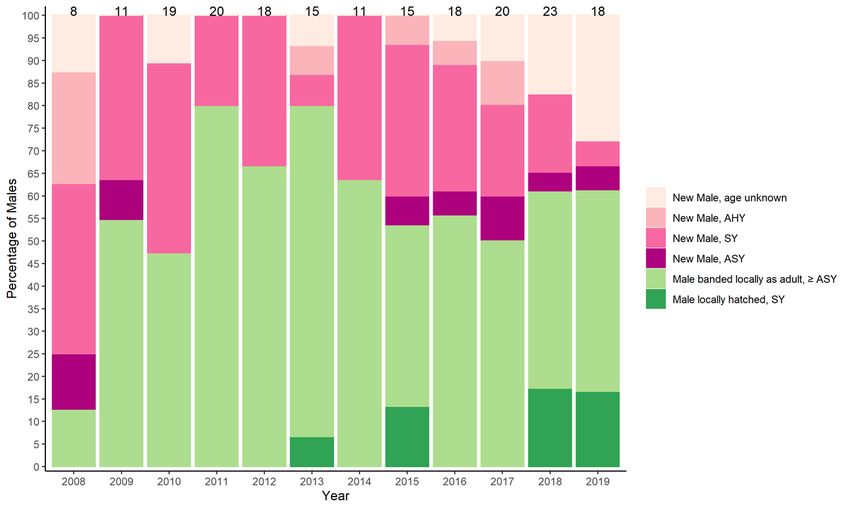
Of males observed in Adams County from 2008 to 2019, 58%
(min = 25%, max = 80%) were after second-year males (hatched
at least two years previous), 30% (min = 13%, max = 47%) were
second-year males (hatched the previous year), and 12% (min =
0%, max = 38%) were of unknown age (Fig. A1.1).
Average density of trees within territories (1577 trees ha-1) was
greater than outside of territories in the same patch (1094 trees
ha-1; Fig. 4). Red pine occurred at greatest density both in
territories (1292 trees ha-1, n = 331) and outside of territories (885
trees ha-1, n = 284), followed by jack pine (territories = 265 treesAvian Conservation and Ecology 17(1): 3
http://www.ace-eco.org/vol17/iss1/art3/
Table 3. Kirtland’s Warbler (Setophaga kirtlandii) nest site habitat use in Adams County, Wisconsin, 2015–2017. We show only the
confidence set models (< 2 AICc from minimum AICc model) ranked by differences in Akaike’s information criterion corrected for
small sample sizes (∆AICc). Column k indicates number of model parameters, wi indicates Akaike weight, AUC is the area under the
receiver operator curve, and R² is the generalized R² (Nakagawa and Schielzeth 2013). Evidence ratios (Ev. Ratio) are the ratio of w1/
wi where model 1 has the lowest AICc and i indexes the rest of the models in the set. Variables marked with an asterisk(*) were considered
to be significant at α = 0.1.
†
k ∆AICc wi Ev. AUC R²
Ratio
Vegetation-height Density 1.25* + Dead Vegetation Depth* + Tree Branch Cover 50%
Vegetation-height Density 1.25* + Vegetation-height density 4.1 + Dead Vegetation Depth* + Tree 5 1.68 0.15 2.3 0.99 0.95
Branch Cover < 50%* + Tree Branch Cover > 50%
†
Minimum AICc value = 30.3
In predicting whether points were within or outside of territories, 1975, Kelly and DeCapita 1982, Bocetti 1994, Rockwell et al.
distance to the nearest tree (which characterizes tree density of 2012) were comparable in the peripheral and core populations.
the entire territory [AO, AP, personal observation]) discriminated This suggests that nesting success is not reduced in red pine-
most strongly (variable importance [VI] value = 0.92); the shorter dominated plantations.
the distance, the greater the probability a point was within a
Although Kirtland’s Warbler nests were closer to red pines than
territory. Vegetation height density 1.25 (VI value = 0.80), and
to other tree species, nests were placed directly in grass, blueberry,
vegetation-height density 1.1 (VI = 0.70; Table 1) were also
or red pine duff and rarely directly under low live tree branches.
important discriminators (Table 4). The predicted probability of
In Michigan, nests were typically placed in open areas of low
a point being within a territory increased from 0.38 to 1.0 when
vegetation within one meter of a pine thicket (Bocetti et al. 2020),
vegetation-height density 1.25 increased from 0 cm to 150 cm
with vegetation directly covering nests mainly composed of
while other variables were held constant at their mean. The
grasses, sedges, and blueberry (Mayfield 1960). Nest sites had
probability of a point being within a territory decreased from 0.83
deeper dead herbaceous vegetation, greater vegetation height-
to 0.04 when vegetation-height density 1.1 increased from 0 cm
density, and greater cover of low tree branches within 0.5 m of
to 133 cm while other variables were held at their mean. The
the nest than non-nest points, suggesting that concealment of
probability of a point being within a territory decreased from 0.89
nests by vegetation, even if not touching the nest, is important.
to 0.05 when average distance to the nearest tree increased from
Perhaps this is because Kirtland’s Warblers use surrounding
1.8 m to 5.4 m while other variables were held at their mean.
vegetation to conceal their nest approaches (Mayfield 1960). Tall
Between territory and random points, we found no difference in dense vegetation may offer nest concealment from predators or
the proportion of points in which the nearest tree was red pine, shelter from the elements (Martin and Roper 1988, Nelson and
jack pine, or oak (chi-square test, χ = 0.4, P = 0.8). Red pine was Martin 1999, Davis 2005, Warren and Anderson 2005, Fisher and
the closest tree at 77–80% of points, jack pine was the closest tree Davis 2010). Dead vegetation is also likely a primary source of
at 19–21% of points, and oak was the closest tree at 1–2% of nest cover early in the season before full green up (Mayfield 1960,
points. Davis 2005, Warren and Anderson 2005, Fisher and Davis 2010).
Many Kirtland’s Warbler nests are built before ground vegetation
Occupied patches has fully emerged; thus females may select sites with high
On average, occupied patches consisted of 70% red pine, 28% jack proportions of dead vegetation because of benefits (concealment,
pine, and 2% oak. Average tree height in occupied patches was thermal etc.) those features may confer. We collected vegetation
4.1 m (SD = 1.1 m, n = 2552 trees) and was identical for red and data after a nesting effort ended regardless of nest fate. This
jack pine, n = 2138 and 391 respectively), while the average height delayed measurement may have resulted in measuring conditions
of oaks was 2.8 m (SD = 1.5, n = 13). Low live branch height of other than what the birds experienced at nest initiation, leading
red pines was closer to the ground (mean = 8.7 cm, SD = 11.6, n to spurious conclusions (McConnell et al. 2017), although we
= 2138) than jack pine (mean = 51.4 cm, SD = 46.0, n = 391). note that vegetative growth rates slowed considerably as the
Mean tree density in occupied patches was 1937 trees ha-1 (SD = summer progressed, mitigating differences in time of use versus
912 trees ha-1, n = 8 patches). time of measurement.
We found that occupied red pine-dominated plantations in Adams
DISCUSSION County had similar proportions of pine (~90% pine; in MI up to
In a population of Kirtland’s Warblers breeding at the range
20% broadleaf; Smith 1979, Probst 1988) but lower densities of
periphery in red pine-dominated plantations, a relatively little
trees (1860 trees ha-1) than jack pine plantations used by Kirtland’s
used habitat type, nesting success was similar to that in long-
Warblers in Lower Michigan (2000–3345 jack pine ha-1; Bocetti
occupied jack pine habitat used by the core population. Both nest
1994, Houseman and Anderson 2002). Additionally, live red pine
survival (WI = 0.43, all years combined; MI = 0.32, Bocetti et al.
branches were nearer to the ground than live jack pine branches
2020) and average number of young fledged per nest (Wisconsin,
in our study site, which could explain why Kirtland’s Warblers
2.5–2.8, 2015–2017; Michigan, 2.8–3.6; Shake and Mattsson
would occupy lower density red pine plantations.Avian Conservation and Ecology 17(1): 3
http://www.ace-eco.org/vol17/iss1/art3/
Table 4. Male Kirtland’s Warbler (Setophaga kirtlandii) territory use in Adams County, Wisconsin, 2016–2017. We show only the
confidence set models (< 2 AICc from minimum AICc model) ranked by differences in Akaike’s information criterion corrected for
small sample sizes (∆AICc). Column k indicates number of model parameters, wi indicates Akaike weight, AUC is the area under the
receiver operator curve, and R² is the generalized R² (Nakagawa and Schielzeth 2013). Evidence ratios (Ev. Ratio) are the ratio of w1/
wi where model 1 has the lowest AICc and i indexes the rest of the models in the set. Variables marked with an asterisk(*) were considered
to be significant at α = 0.1.
†
k ∆AICc wi Ev. AUC R²
Ratio
Vegetation-height density 1.25* + Vegetation-height density 1.1* + tree distance* 3 0 0.12 0.83 0.68
vegetation-height density 1.25* + vegetation-height density 1.1* + vegetation-height density 4.25 + 4 1.56 0.06 2.18 0.83 0.65
tree distance*
vegetation-height density 1.25* + vegetation-height density 1.1* + shrub distance + tree distance* 4 1.73 0.05 2.38 0.83 0.68
†
Minimum AICc value = 70.33
Within occupied patches, territories had slightly greater tree quality to jack pine plantations in the core range. However, we
density than random locations (~480 trees ha-1 greater). Relative cannot rule out the possibility that newly arrived after-second-
frequencies of red and jack pine were not different between year birds in Adams County were subordinate to territory holders
territories and random locations. If males were using jack pine in in the core habitat, as metrics associated with dominance were
greater proportion than was present in occupied patches, not measured.
territories should have a higher proportion of jack pine than
Demographic rates are often hypothesized to be greatest at a
locations outside of territories. Point level measures of distance
species’ geographic range center, coinciding with peak species
to trees (our proxy of point-level tree density) indicates that trees
abundance, and lowest at the range periphery. This pattern is
within territories are closer together than trees outside of
found in multiple species (Wright et al. 2007, Hollander et al.
territories. On territories, vegetation-height density measured at
2011, Golawski et al. 2016). However, demographic rates are not
0.25 m height was greater than in areas outside of territories but
always greater at the core of a species’ range. Local habitat quality
within the same patch, suggesting that males establish territories
may more strongly influence fecundity across geographic ranges
in areas with greater low vegetation cover, possibly because it
than large scale environmental gradients (Pidgeon et al. 2001,
offers better foraging opportunities, more potential nest sites, or
Hargrove and Rotenberry 2011, Ruskin et al. 2017). Or there may
lower detection by predators. However, we also found that
be no differences in reproductive success between populations
territories had lower vegetation-height density measured at 1 m
across a geographic range (Barrientos et al. 2009). Kirtland’s
height than outside of territories. It is less clear why this negative
Warblers align with this latter group, in that nest survival rates
association exists with density of tall vegetation, but we speculate
and number of young fledged per nest in peripheral habitat and
that dense tall grass may be more difficult for Kirtland’s Warblers
the core of the breeding range are similar.
to fly through. Although we expected blueberry cover to be an
important habitat feature, we did not find that to be the case. In response to habitat creation and Brown-headed Cowbird
Although blueberry cover may be important for foraging control, the Kirtland’s Warbler population has recovered and is
opportunities or nest concealment, it is possible that at scales no longer listed as federally endangered (Federal Register 2019).
larger than the nest site Kirtland’s Warblers may accept a wide A goal stated in the Kirtland’s Warbler Conservation Plan is to
range of ground cover compositions (Probst 1988, Probst and provide suitable breeding habitat in areas peripheral to the core
DonnerWright 2003). It is also possible that blueberry is range for 10% (100 pairs) of the Kirtland’s Warbler population
unimportant on territories because fruiting does not occur until (Michigan Department of Natural Resources et al. 2015).
territories begin to break down as the nesting period ends. Kirtland’s Warblers will always remain conservation-reliant
because wildfire suppression prevents natural habitat creation,
The population of Kirtland’s Warblers in Adams County is likely
and cowbird parasitism depresses their productivity. The
still growing. All suitable territories in occupied plantations may
challenge in the post-delisting period is to continue creating
not be filled, nor all suitable habitat patches occupied. The
suitable breeding habitat and managing Brown-headed Cowbirds.
contrast in habitat attributes between territory and non-territory
Although Kirtland’s Warblers in the core range appear to be
points may be subtle if non-territory points are also suitable but
resilient to relaxed levels of cowbird control (Cooper et al. 2019),
unoccupied (Fretwell and Lucas 1969, Fretwell 1972, Hartman
the small population in Adams County suffers from high levels
1996). Conspecific attraction also influences habitat occupancy
of brood parasitism even with active cowbird management and
in Kirtland’s Warblers (Mayfield 1960, Bocetti 1994, Anich and
a declining Brown-headed Cowbird population in Wisconsin
Ward 2017), and likely enhances suitability of occupied patches
(-2.67% over the period 2007–2017, North American Breeding
through (positive) Allee effects (Allee et al. 1949). If red pine-
Bird Survey, Patuxent Wildlife Research Center-Bird Population
dominated habitat in Adams County was of marginal quality, we
Studies, https://www.mbr-pwrc.usgs.gov/). The cowbird population
would expect most new males observed each year to be second
trend is comparable to that in Michigan over this same 10-year
year birds or birds that were subordinate. We did not find evidence
period (-3.06%, ibid). Low parasitism rates in Michigan are
of this. Most newly observed males were after-second-year birds,
attributed to low cowbird population size, associated with
suggesting that red pine plantations are perceived to be of similar
reforestation (Cooper et al. 2019); however, in Adams CountyAvian Conservation and Ecology 17(1): 3
http://www.ace-eco.org/vol17/iss1/art3/
WI, agriculture is prevalent, which could account for the
differences in nest parasitism rates in the two states.
Managers will likely need to minimize costs associated with LITERATURE CITED
creating Kirtland’s Warbler habitat, and managers in Wisconsin Allee, W. C., A. E. Emerson, O. Park, T. Park, and K. P. Schmidt.
will likely need to continue managing cowbirds. One option for 1949. Principles of animal ecology. Saunders, Philadelphia,
increasing timber value is inter-planting red and jack pine trees Pennsylvania, USA.
in plantations, a strategy included in the most recent Kirtland’s Anich, N. M., J. A. Trick, K. M. Grveles, and J. L. Goyette. 2011.
Warbler Conservation Plan (Michigan Department of Natural Characteristics of a red pine plantation occupied by Kirtland’s
Resources et al. 2015). Warblers in Wisconsin. Wilson Journal of Ornithology
Our findings, together with others from red pine-dominated 123:199-205. https://doi.org/10.1676/10-057.1
plantations (Anich et al. 2011, Richard 2014), suggest that suitable Anich, N. M., and M. P. Ward. 2017. Using audio playback to
Kirtland’s Warbler breeding habitat can consist of various expand the geographic breeding range of an endangered species.
combinations of red pine and jack pine in a managed plantation. Diversity and Distributions 23:1499-1508. https://doi.org/10.1111/
When the Kirtland’s Warbler population was lowest, management ddi.12635
focused on habitat known to sustain the population: young jack
pines intermixed with grassy openings. Now that the species is no Arnold, T. W. 2010. Uninformative parameters and model
longer threatened with extinction, managers have more flexibility selection using Akaike’s Information Criterion. Journal of
to plant a range of tree species composition proportions that Wildlife Management 74:1175-1178. https://doi.org/10.2193/2009-367
Kirtland’s Warblers will use as breeding habitat, which may
facilitate lower costs of managing habitat for this conservation- Barbosa, A. M., J. A. Brown, A. Jiménez-Valverde, and R. Real.
reliant species. 2016. modEva: Model evaluation and analysis. [online] URL:
http://hdl.handle.net/10174/20946
Barrientos, R., A. Barbosa, F. Valera, and E. Moreno. 2009.
Responses to this article can be read online at: Breeding parameters of the Trumpeter Finch at the periphery of
https://www.ace-eco.org/issues/responses.php/2009 its range: a case study with mainland expanding and island
populations. Journal of Arid Environments 73:1177-1180. https://
doi.org/10.1016/j.jaridenv.2009.06.001
Author Contributions: Bartoń, K. 2018. MuMIn: multi-model inference. [online] URL:
All authors conceptualized the project, designed the research, and https://cran.r-project.org/web/packages/MuMIn/index.html
participated in writing and editing. AO collected and formally Battin, J., and J. J. Lawler. 2006. Cross-scale correlations and the
analyzed the data, and wrote the original draft. AP and CR design and analysis of avian habitat selection studies. Condor
participated in analysis of the data, reviewing and editing, and 108:59-70. https://doi.org/10.1093/condor/108.1.59
funding acquisition for the project. KG, DL, and SW assisted with
project logistics. Bocetti, C. I. 1994. Density, demography, and mating success of
Kirtland’s Warblers in managed and natural habitats.
Dissertation. Ohio State University, Columbus, Ohio, USA.
Acknowledgments: [online] URL: http://rave.ohiolink.edu/etdc/view?acc_num=
This work was supported by the National Science Foundation osu1487856076416827
Graduate Research Fellowship (Grants. DGE-1256259 and Bocetti, C. I., D. M. Donner, and H. F. Mayfield. 2020. Kirtland’s
DGE-1747503), and the National Institute of Food and Warbler (Setophaga kirtlandii), version 1.0. In A. F. Poole, editor.
Agriculture, USDA (grant number WIS01590). Funding was Birds of the World. Cornell Lab of Ornithology, Ithaca, New
provided to A.O. by the American Ornithologists Union, the York, USA. https://doi.org/10.2173/bow.kirwar.01
Association of Field Ornithologists, and the Wisconsin Society for
Ornithology. No funder had input into the content of the manuscript. Braillet, C., A. Charmantier, F. Archaux, A. Dos Santos, P. Perret,
We thank the Natural Resources Foundation of Wisconsin for and M. M. Lambrechts. 2002. Two Blue Tit Parus caeruleus
assistance. Thank you, J. Cummings, K. Reinstma, L. White, N. populations from Corsica differ in social dominance. Journal of
Anich, L. Serna, Z. Osberg, and A. Jocham for help with data Avian Biology 33:446-450. https://doi.org/10.1034/j.1600-048X.2002.02956.
collection. Thank you, N. Livingston, for being a long-time friend x
of Kirtland’s Warblers and providing housing. We thank C. Bocetti, Brown, J. H. 1984. On the relationship between abundance and
D. Donner, R. White, for comments on previous manuscript versions. distribution of species. American Naturalist 124:255-279. https://
Use of trade, firm, or product names is for descriptive purposes only doi.org/10.1086/284267
and does not imply endorsement by the U.S. Government. Findings
and conclusions in this article are those of the authors and do not Buech, R. R. 1980. Vegetation of a Kirtland’s Warbler breeding
necessarily represent the views of USFWS. All activities were area and 10 nest sites. Jack-Pine Warbler 58:58-72.
approved under the following permits or protocols: USFWS Burnham, K. P., and D. R. Anderson. 2004. Multimodel
Endangered Species Recovery Permit TE99059B-2, WDNR inference: understanding AIC and BIC in model selection.
Endangered and Threatened Species Permit #1052, USGS Federal Sociological Methods and Research 33:261-304. https://doi.
Bird Banding permit #23398, and University of Wisconsin - org/10.1177/0049124104268644
Madison Animal Care and Use Protocol A005409.You can also read