Quantifying Southern Annular Mode paleo-reconstruction skill in a model framework
←
→
Page content transcription
If your browser does not render page correctly, please read the page content below

Clim. Past, 17, 1819–1839, 2021
https://doi.org/10.5194/cp-17-1819-2021
© Author(s) 2021. This work is distributed under
the Creative Commons Attribution 4.0 License.

Quantifying Southern Annular Mode paleo-reconstruction skill
in a model framework
Willem Huiskamp1,2 and Shayne McGregor3
1 RD1 – Earth System Analysis, Potsdam Institute for Climate Impact Research (PIK), Member of the Leibniz Association,
Potsdam, Brandenburg, Germany
2 Climate Change Research Centre, UNSW Sydney, Sydney, NSW, Australia
3 School of Earth Atmosphere and Environment, Monash University, Melbourne, Victoria, Australia

Correspondence: Willem Huiskamp (huiskamp@pik-potsdam.de)

Received: 13 October 2020 – Discussion started: 20 October 2020
Revised: 23 July 2021 – Accepted: 26 July 2021 – Published: 13 September 2021

Abstract. Past attempts to reconstruct the Southern Annular         and precipitation in Australia (Hendon et al., 2007), New
Mode (SAM) using paleo-archives have resulted in records            Zealand (Gallant et al., 2013), as well as South America
which can differ significantly from one another prior to the        and Africa (Gillet et al., 2006; Silvestri and Vera, 2009).
window over which the proxies are calibrated. This study            For example, positive phases of the SAM over the period
attempts to quantify not only the skill with which we may           1979–2005 are typically associated with cool annual tem-
expect to reconstruct the SAM but also to assess the con-           perature anomalies over the Antarctic continent (Thompson
tribution of regional bias in proxy selection and the impact        and Solomon, 2002; Kwok and Comiso, 2002; Gillet et al.,
of non-stationary proxy–SAM teleconnections on a resulting          2006) and warm anomalies over the Antarctic Peninsula,
reconstruction. This is achieved using a pseudoproxy frame-         southern South America, and southern New Zealand (Kwok
work with output from the GFDL CM2.1 global climate                 and Comiso, 2002; Silvestri and Vera, 2009). Precipitation
model. Reconstructions derived from precipitation fields per-       changes typically found during a positive SAM phase include
form better, with 89 % of the reconstructions calibrated over       negative annual precipitation anomalies over southern South
a 61 year window able to reproduce at least 50 % of the inter-      America, New Zealand, and Tasmania, as well as positive
annual variance in the SAM, as opposed to just 25 % for             precipitation anomalies over Australia and South Africa (Sil-
surface air temperature (SAT)-derived reconstructions. Non-         vestri and Vera, 2009).
stationarity of proxy–SAM teleconnections, as defined here,            Over the last five decades, the SAM has shown a trend
plays a small role in reconstructions, but the range in re-         towards more positive values, consistent with a poleward in-
construction skill is not negligible. Reconstructions are most      tensification of the surface westerly winds, which has been
likely to be skilful when proxies are sourced from a geo-           largely attributed to anthropogenic forcing, such as strato-
graphically broad region with a network size of at least 70         spheric ozone depletion and the increase in atmospheric
proxies.                                                            CO2 (Son et al., 2008; Lee and Feldstein, 2013; Previdi
                                                                    and Polvani, 2014). In addition, both high-frequency (3–4
                                                                    months) and low-frequency (16 years) variability, as derived
                                                                    from reanalysis experiments, has been observed in the SAM
1   Introduction                                                    (Raphael and Holland, 2006). It is important to place these
                                                                    observed trends over the last five decades into a long-term
The Southern Annular Mode (SAM), which describes the in-            context in order to understand the contributions of forced
tensity and latitudinal location of the subtropical westerly jet,   and natural variability. These relative contributions are im-
is the leading mode of atmospheric variability in the South-        portant for understanding projected future changes, given the
ern Hemisphere. Positive and negative phases of the SAM             impact of the SAM on not only regional weather patterns but
have been linked to changes in surface air temperature (SAT)

Published by Copernicus Publications on behalf of the European Geosciences Union.
1820                                                    W. Huiskamp and S. McGregor: Quantifying SAM reconstruction skill

also large-scale ocean circulation and heat uptake (Russell       tionately on records from narrow longitude bands. Sites are
et al., 2006; Marini et al., 2011; Liu et al., 2018) and even     primarily in South America, Australia and New Zealand (Vil-
the marine carbon cycle (Lovenduski et al., 2007; Lenton and      lalba et al., 2012), and Antarctica (Zhang et al., 2010; Abram
Matear, 2007; Le Quéré et al., 2007; Huiskamp and Meiss-          et al., 2014; Dätwyler et al., 2018), with Antarctica being
ner, 2012; Hauck et al., 2013; Huiskamp et al., 2016; Keppler     the only location that is able to provide samples with good
and Landschützer, 2019).                                          longitudinal coverage. Abram et al. (2014) show that their
   Instrumental reconstructions of the SAM extend as far          regional Drake Passage sector paleo-reconstruction of the
back as 1865 (Jones et al., 2009), but those for periods prior    SAM is representative of the hemispheric mean signal by ex-
to the mid-twentieth century involve significant uncertainty      tracting a sea level pressure-derived (SLP) SAM index from
due to fewer observations and the methods used to compen-         a suite of eight global climate models and comparing it with
sate for this (i.e. estimates based on atmospheric conserva-      a secondary SAM index derived from the same SLP field but
tion of mass, e.g. in Jones et al., 2009). Direct measurements,   restricted to the Drake Passage sector. They find that the re-
meanwhile, only extend as far back as 1958 (Marshall, 2003).      gional expression of the SAM in these models closely re-
Thus, if we wish to extend our understanding of SAM trends        sembles the hemispheric expression over 1000 years, a con-
and variability back beyond the instrumental record, recon-       clusion supported by the regional SAM records of Visbeck
structions derived from paleo-archives are required.              (2009). Dätwyler et al. (2018), on the other hand, find non-
                                                                  trivial differences between their hemisphere-wide SAM re-
1.1     Paleo-reconstructions of SAM variations
                                                                  construction and that of Abram et al. (2014), implying that an
                                                                  annual-mean SAM reconstructed from paleo-proxies is not
Paleo-reconstructions are generated by examining changes          well approximated by sampling from a limited region.
preserved in natural environmental archives (biological,             Secondly, when we correlate a proxy with the modern
chemical, and physical records) that are sensitive to climatic    SAM over a calibration window of several decades, we
impacts of the mode of variability being reconstructed. In        make the assumption that this relationship remains the same
the case of the SAM, this has traditionally been achieved         through time. This is commonly referred to as proxy sta-
by finding proxies that are sensitive to precipitation or sur-    tionarity. Gallant et al. (2013) investigated SAT/precipitation
face air temperature changes associated with the two dif-         non-stationarity using instrumental data spanning the period
ferent phases of the SAM. Proxies that record changes in          1900–2009 and reported that 21 %–37 % of Australian pre-
temperature and precipitation include tree rings, ice cores,      cipitation records showed non-stationary teleconnections to
and terrestrial sediment cores, although the latter are less      the El Niño–Southern Oscillation (ENSO) and the SAM. Sil-
favoured due to chronological uncertainties and, typically, a     vestri and Vera (2009) performed a similar study with ob-
lower temporal resolution. Tree growth, and therefore ring        served precipitation and surface air temperature records for
width and/or density, can be sensitive to both temperature        the spring months in Australia and South America span-
and precipitation depending on the tree type and its location,    ning the 1960s/1970s and the 1980s/1990s. They found that
while ice cores can provide accumulation rates, δ 18 O and δD     significant positive correlations of the SAM with SAT in
(e.g. Steig et al., 2005), which record air temperature and       the Australia/New Zealand region in the earlier decades
precipitation (accumulation).                                     could become insignificant or even negative in more recent
                                                                  decades. Dätwyler et al. (2018) built on this by adding sta-
1.1.1    Reconstructions and their potential issues
                                                                  tionarity criteria to their proxies for reconstructing the SAM,
                                                                  but at a cost of calibrating their proxies with a longer but less
The relationship to the SAM is typically initially established    reliable record (Jones et al., 2009). The resulting reconstruc-
by correlating changes in these proxy records with a SAM          tions showed a more stable teleconnection through time but
index developed from instrumental or reanalysis data over         were not necessarily more skilful (as measured by validation
a period spanning several decades (Villalba et al., 2012 and      statistics). Finally, when considering multi-decadal calibra-
references therein; Abram et al., 2014). The individual proxy     tion periods, stochastic noise or other climate signals (e.g.
records are then combined into a single index using a recon-      ENSO) can modulate the correlation strength between, for
struction method such as a regression approach (Zhang et al.,     example, South American precipitation and the SAM with-
2010; Villalba et al., 2012) or weighted composite plus scal-     out the precipitation record being classified as non-stationary
ing (CPS; Abram et al., 2014; Dätwyler et al., 2018).             (Yun and Timmermann, 2018).
   However, two fundamental assumptions are being made               This study aims to quantify the uncertainties raised by
when we reconstruct the past climate in this way. Firstly,        the aforementioned assumptions within a modelling frame-
we assume that a hemisphere-wide mode of variability can          work, similar to Batehup et al. (2015), and seeks to address
be accurately reconstructed using records from a geograph-        the following questions: (1) What impacts do the proxy net-
ically limited sample space. As there is relatively little land   work size and calibration window size have on the skill of
in the Southern Hemisphere, particularly in the latitude of       a resulting reconstruction? (2) How does the geographical
the westerlies, SAM reconstructions often rely dispropor-         distribution of the proxies affect reconstruction skill? (3)

Clim. Past, 17, 1819–1839, 2021                                                      https://doi.org/10.5194/cp-17-1819-2021
W. Huiskamp and S. McGregor: Quantifying SAM reconstruction skill                                                          1821

Are any regions in our model framework prone to produc-          plitude of the model’s SAM index is comparable with obser-
ing non-stationary proxies, and what could be modulating         vations (Raphael and Holland, 2006), although its variability
the SAM–proxy teleconnection? The use of climate models          is larger than observed (Karpechko et al., 2009). As previ-
to assess the paleo-reconstruction skill provides an oppor-      ously noted, we should be cautious about directly comparing
tunity to investigate a “perfect” time series of the climate     observations spanning a brief time period (in this instance,
index we wish to reconstruct and the ability to reconstruct      ERA-Interim (Dee et al., 2011) data correlated with the Mar-
this index with fields from a model that act as pseudopaleo-     shall SAM index (Marshall, 2003) over the 36 year period
proxies (Mann and Rutherford, 2002; Mann et al., 2007).          1979–2014) for which there is a well-observed SAM trend
These “perfect” proxies are free from non-climatic noise that    with our model data, which represents a stable pre-industrial
may degrade a teleconnection signal between a real proxy         climate spanning 500 years. To address this, we calculate a
and the SAM. Instead, our pseudoproxies isolate changes          36 year running correlation between the model SAM and our
in teleconnection strength due to underlying variability in      SAT and precipitation fields and identify whether the corre-
the climate only. This is in contrast to “real world” prox-      lations derived from observations fall within the model range
ies, which are also prone to other influences inherent to the    (Fig. 1). The SAM index in the model is calculated accord-
physical/chemical/biological nature of the proxy itself. It is   ing to the method of Gallant et al. (2013) as the difference
often assumed that these effects will be minimised by sam-       in normalised, zonally averaged sea level pressure anomalies
pling proxies from a range of regions, as local factors from     between 40 and 60◦ S. Except in a region of equatorial South
different locations would not be expected to be correlated.      America in the SAT field, the agreement is good, with 87 %
Additionally, model data allow us to assess multi-decadal to     of the SAT and 95 % of the precipitation grid cells on land
centennial changes in proxy–SAM teleconnection and how           showing agreement with observations.
calibration over certain windows in time affects the skilful-       Paleo-proxies are not uniformly sensitive to one season or
ness of a SAM reconstruction.                                    variable; their sensitivities depend on the region from which
                                                                 they are sourced. For example, a tree ring record constructed
                                                                 by Cullen and Grierson (2009) from south-west Western
2     Methods
                                                                 Australia was shown to be particularly sensitive to austral
2.1    Model and data
                                                                 autumn–winter precipitation. Alternatively, South American
                                                                 tree ring records compiled by Villalba et al. (2012) show sen-
The data used in this study are a 500-year pre-industrial con-   sitivity to summer–autumn precipitation, while New Zealand
trol simulation of the Geophysical Fluid Dynamics Labora-        records appear to be most responsive to summer temperature.
tory’s Coupled Model 2.1 (CM2.1 hereafter), with all bound-      In addition, while the proxies are sensitive to SAT or precipi-
ary conditions set to CE 1860 levels. This assures that any      tation during one season, the strongest influence of the SAM
changes in the model SAM are due to internal variability in      on these variables may occur during a different season en-
the climate system only. CM2.1 is a fully coupled global cli-    tirely. For example, while the South American tree rings of
mate model with ocean (OM3.1), atmosphere (AM2.1), land          Villalba et al. (2012) are sensitive to summer–autumn pre-
(LM2.1), and sea-ice (SIS) components. The ocean model           cipitation, the SAM signal is most clearly seen in late spring
has a resolution of 1◦ × 1◦ , which increases equatorward        and winter precipitation in south-eastern South America (Sil-
from 30◦ latitude to a meridional resolution of 1/3◦ at the      vestri and Vera, 2009). With this in mind, we employ annual
equator (Griffies et al., 2005). The atmospheric and land sur-   mean (January–December) fields for sea level pressure, sur-
face models have a resolution of 2◦ latitude by 2.5◦ longi-      face air temperature, and precipitation for the following rea-
tude, and the AM2.1 has 24 vertical levels (Delworth et al.,     sons: (1) the CMIP5 generation of models (including CM2.1)
2006).                                                           are less skilful at representing the seasonal variability in the
   CM2.1 is selected due to its good representation of the       SAM–SAT relationship than they are at representing the an-
SAM compared to similar models from the CMIP5 and                nual mean (Marshall and Bracegirdle, 2015); (2) reconstruct-
CMIP6 archives (Bracegirdle et al., 2020), while Karpechko       ing the SAM on an annual-mean timescale should smooth out
et al. (2009) find its performance to be favourable when com-    high-frequency noise in the proxies and enhance the signal-
pared to ERA-40 data. The spatial structure of the SAM is        to-noise ratio of our reconstructions; and (3) it enables us to
well simulated, accurately capturing the centre of action over   simplify the experimental parameter space and focus instead
the Pacific while being slightly too zonally symmetric in the    on the impacts of network size and calibration window length
eastern half of the Southern Hemisphere (Raphael and Hol-        rather than seasonal effects.
land, 2006). Importantly for our purposes, CM2.1 accurately
simulates the latitude at which the SAM transitions from         2.2   Calculation of non-stationarity
its positive to its negative phase (as expressed via regres-
sion onto 850 hPa winds) over South America, which many          A proxy is typically considered non-stationary if its telecon-
models of a similar age and computational complexity fail to     nection to the SAM is changed by a dynamical process rather
achieve (Raphael and Holland, 2006, their Fig. 4b). The am-      than stochastic variability (localised weather), such that the

https://doi.org/10.5194/cp-17-1819-2021                                                     Clim. Past, 17, 1819–1839, 2021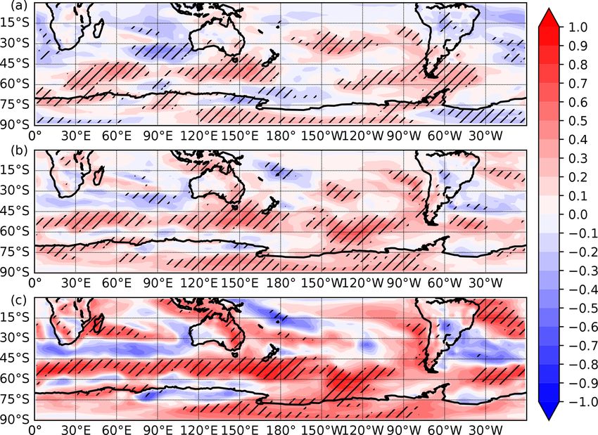
1822                                                       W. Huiskamp and S. McGregor: Quantifying SAM reconstruction skill

Figure 1. Correlations of annual-mean (January–December) SAT (a) and precipitation (b) from the GFDL CM2.1 model with the model-
derived SAM, calculated over 500 years. Black dots show where the correlation of the ERA-Interim reanalysis product with the Marshall
SAM index, calculated over a 36 year period from 1979 to 2014, does not fall within the range of the model’s 36 year running correlation at
each grid cell.

signal it records no longer represents changes in the SAM.              SAT/precipitation time series and the SAM index. The red
Here, the SAM teleconnection is modelled via a running cor-             noise is a combination of random Gaussian noise (ηv (t))
relation between the proxy and the SAM index over a win-                and the autocorrelation (β) of the SAT or precipitation time
dow of 31, 61, or 91 years. We define non-stationary telecon-           series at a lag of 1 year multiplied by the Gaussian noise
nections following the method of Gallant et al. (2013) and              (βηv (t − 1)).
Batehup et al. (2015), such that a proxy is considered non-                The stochastic simulations of SAT and precipitation are
stationary when the variability in its running correlation with         used to create a 95 % confidence interval for each grid point
the SAM exceeds what would be expected if the proxy were                of all possible running correlations a time series could have
only influenced by local random noise.                                  and still be considered to have a stationary teleconnection
   Following on from this, a Monte Carlo approach (van Old-             with the SAM. Therefore, if the time series from our model
enborgh and Burgers, 2005; Sterl et al., 2007; Gallant et al.,          proxy has a running correlation that falls outside the confi-
2013) is used to create stochastic simulations of SAT and pre-          dence interval, we consider that proxy to be non-stationary
cipitation at each grid point in the model. These stochastic            with the SAM in that temporal window, as it is unlikely to be
simulations are created to have the same statistical properties         affected by stochastic processes alone. It should be noted that
as the original SAT and precipitation data from the CM2.1               as a 95 % confidence interval is used, non-stationarity will
simulation. To determine the range of variability expected              be falsely identified 5 % of the time, hence we define a grid
due to the stochastic processes mentioned previously, 1000              point as non-stationary only if the running correlation falls
of these time series are created at each grid point according           out of the confidence interval more than 10 % of the time –
to the following equation from Gallant et al. (2013):                   more than double the 5 % we might expect by chance alone.
                         p                                              The running correlations are converted to Fisher Z-scores to
v(t) = a0 + a1 c(t) + σv 1 − r 2 [ηv (t) + βηv (t − 1)].    (1)         ensure they are normally distributed for the calculation of
                                                                        confidence intervals:
Here, v(t) is the stochastic SAT or precipitation time series,
                                                                              1     1+r
a0 and a1 are regression coefficients representing the station-         Z = ln              ,                                       (2)
ary teleconnection strength between the SAT or precipita-                     2     1−r
tion and the SAM index (c(t)), while the remaining terms                where r is the running correlation value.
represent the noise added to the time series. A red noise,
[ηv (t) + βηv (t − 1)], is added and weighted by the standard
                                                                        2.3   Generation of pseudoproxies
deviation σv of the local SAT or precipitation time series as
well as the√proportion of the variance not related to the re-           SAT and precipitation fields from the model are used to rep-
gression ( 1 − r 2 ), where r is the correlation between the            resent climate proxies in the model, as discussed in Sect. 2.1.

Clim. Past, 17, 1819–1839, 2021                                                             https://doi.org/10.5194/cp-17-1819-2021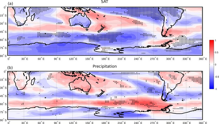
W. Huiskamp and S. McGregor: Quantifying SAM reconstruction skill                                                                 1823

Rather than being inferred via changes in tree ring growth,       Table 1. The range in the number of sites available for use in a SAT
these proxies are direct measures of these variables and there-   or precipitation proxy network in each region and the calibration
fore free of non-climatic noise (von Storch et al., 2009). We     window size. The range was calculated across the 10 different cal-
do not add noise to increase the realism of these proxies;        ibration windows used when creating the network, as discussed in
rather, we assess reconstruction skill and non-stationarity in    Sect. 2.3.
a “best case scenario” where we assume that the proxy is a
                                                                                                             Number of sites
perfect analogue for the climate variable it is deemed to rep-
resent (SAT or precipitation), similar to the experiments of           Region            Window size         SAT        Precip.
Dätwyler et al. (2020).                                                                     31 years      842–1740     549–935
   Proxies are randomly selected in accordance with two con-           S. Hemisphere        61 years      640–1568     429–709
ditions. Ideally, proxies would be calibrated with the SAM                                  91 years      838–1535     326–660
over the full length of the time series (500 years); however,
                                                                                            31 years      557–1346     264–563
as previously noted, real-world proxies are calibrated over
                                                                       Antarctica           61 years      454–1253     191–403
shorter windows of several decades. For each grid point in                                  91 years      705–1254     211–396
the model, the time series is split into 10 windows either 31,
61, or 91 years in length, whose midpoints are evenly spaced                                31 years       48–152       60–166
throughout the 500 years regardless of the overlap or space            Aus./NZ              61 years       41–130       46–165
between them. A proxy may be selected if it is (1) on land                                  91 years       31–132       33–158
in the Southern Hemisphere and (2) has a correlation with                                   31 years       54–244       62–195
the model SAM index of |0.3| or greater within the calibra-            S. America           61 years       44–227       46–156
tion window, after the method of McGregor et al. (2013) and                                 91 years       30–207       39–154
Batehup et al. (2015). A threshold correlation of 0.3 is an
arbitrary choice, but it ensures that the proxy represents the
SAM to some extent while not being so high that proxies are
only sourced from a geographically limited region.                (PAGES 2k Consortium, 2013; Abram et al., 2014; Bate-
   The number of proxies that meet our criteria in each re-       hup et al., 2015; Dätwyler et al., 2018). Using this method,
gion/window size is shown in Table 1. This approach allows        proxies are normalised to have a zero mean and unit stan-
for the possibility that a proxy has a strong correlation with    dard deviation, and are then weighted according to their cor-
the SAM over the selected calibration window but an in-           relation with the model SAM over the calibration window
significant or even reversed correlation over other windows,      before being summed into a single time series. To quantify
or indeed the full 500 years. The window sizes were chosen        the skill of the pseudoproxy reconstructions, Pearson correla-
to assess the effect of window length on the resulting skill of   tion coefficients between each normalised SAT/precipitation-
the reconstruction. For example, the use of a 61 year calibra-    derived SAM index and the sea level pressure-derived SAM
tion window, as opposed to a 31 year one, may decrease the        index over the full 500 years of data are calculated. We de-
effect of decadal climate variability and its modulation of the   fine a skilful reconstruction as one that is able to reproduce
pseudoproxy–SAM teleconnection.                                   at least 50 % of the model SAM variability (i.e. r 2 ≥ 0.5 or
   Reconstructions are computed with a network size of be-        r ≥∼ 0.71).
tween 2 and 70 proxies, a range typical of past reconstruc-          To investigate the role that ENSO may play in modulating
tions with strict selection criteria (e.g. Abram et al., 2014     the pseudoproxy–SAM teleconnection, a correlation coeffi-
and Dätwyler et al., 2018). This is done to quantify the de-      cient is calculated between the running correlation time se-
pendence of reconstruction skill on network size. 1000 net-       ries of SAM-SAT/precipitation and the model Nino3.4 (n3.4)
works are generated for each of the 10 calibration windows        index at each grid point. The n3.4 index is chosen due to
for each network size. Each site in each network is randomly      its optimal representation of the character and evolution of
selected and unique, while the same site may be included          El Niño and La Niña events (Bamston et al., 1997; Trenberth
in more than one network. Similarly, all sites in a network       and Stepaniak, 2001). The model n3.4 index is calculated as
are selected based upon correlations over a single window         the sea surface temperature anomaly in the region from 5◦ N
and may therefore be absent from networks calibrated using        to 5◦ S and from 170◦ W to 120◦ W.
a different window.                                                  Each SAT and precipitation grid cell is correlated with the
   To reconstruct the proxy networks into a single proxy-         SAM over a 31, 61, and 91 year running window, while the
SAM index, we use the weighted composite plus scale (CPS)         n3.4 index is bandpass filtered using the same window size
method (Esper et al., 2005; Hegerl et al., 2007), similar to      to remove high-frequency variability. The two time series are
that used by Abram et al. (2014). The scope of this study does    then correlated over their common interval (500 years minus
not include the effects of different reconstruction methods on    the window size), with the significance calculated using a
the skill of the reconstructed index, so we choose to use CPS     reduced degrees of freedom method (Davis, 1976). An addi-
because it is commonly employed in paleo-reconstructions          tional set of SAM reconstructions are calculated which ex-

https://doi.org/10.5194/cp-17-1819-2021                                                        Clim. Past, 17, 1819–1839, 2021
1824                                                    W. Huiskamp and S. McGregor: Quantifying SAM reconstruction skill

clude any proxy whose SAM–proxy running correlation is             proxies and the 31 year window) are r = 0.62 for SAT and
found to have a significant (p < 0.05) correlation to the fil-     r = 0.59 for precipitation, reconstructing 38 % and 35 % of
tered n3.4 index over the relevant calibration window.             the SAM variability, respectively (Fig. 3a and d).
                                                                      The range in reconstruction skill presented in Fig. 3 in-
3     Results                                                      dicates that even when the network size is maximised and a
                                                                   long window is selected, simply calibrating during a different
The importance of a long calibration window is illustrated in      period can change the skill of the resulting reconstruction. It
Fig. 2. For example, a true correlation of −0.3 between pre-       is noteworthy that increasing the calibration window length
cipitation and the SAM may become anything ranging from            does not necessarily increase the maximum possible skill of
−0.65 to 0.1 when evaluated over a shorter 31 year window          the resulting reconstruction, but rather leads to a reconstruc-
(Fig. 2d). However, as the window size increases, it is in-        tion converging towards the skill of a so-called “true” re-
creasingly likely that the calculated correlation is represen-     construction. This true reconstruction utilises the entire time
tative of the true correlation. For example, calibration win-      span of our data for calibration, which is 500 years here, and
dows of 61 and 91 years ensure that our proxy’s correlation        shows the actual ability of these proxies to reconstruct the
with SAM is always the same sign as it is over the 500 year        SAM. This convergence is visible for the SH SAT reconstruc-
period (Fig. 2e and f). Also noteworthy is the considerable        tions (Fig. 4a, e, and i), where a longer calibration window
decrease in the maximum available number of proxies eligi-         does not increase the 95th percentile of reconstruction skill
ble for inclusion in reconstructions when calibrating with a       nor necessarily increase the proportion of skilful reconstruc-
61 year window rather than a 31 year window (Table 1). A           tions (Fig. 4e and i; red lines). In other words, a longer cal-
smaller decrease in the proxy pool is seen when lengthening        ibration window will more realistically represent a proxy’s
the window from 61 to 91 years.                                    relationship with the SAM, but, as a result, it may decrease
                                                                   the skill of the reconstructed SAM.
                                                                      As Antarctica represents a large percentage of the avail-
3.1    Reconstruction skill
                                                                   able proxies (Table 1), reconstructions are included for prox-
Reconstructions of the SAM often rely heavily on proxies           ies sourced from the entire Southern Hemisphere other than
from a very limited geographic location. What follows are          Antarctica to ensure they are not disproportionately impact-
several reconstructions, each one utilising proxies from one       ing the skill of our reconstructions. The Antarctic-free SAT
or more regions which are commonly used to reconstruct             reconstructions are less skilful for the 31 and 61 year win-
the SAM. In the first scenario, shown in Fig. 3a–f, pseu-          dows with a larger range in r. Note that most of the 95th per-
doproxies are sourced from the entire Southern Hemisphere          centile (Fig. 3g, h, i – red shading) is below the r 2 > 0.5 skil-
(SH), including Antarctica. The reconstruction skill is dis-       ful threshold, as opposed to reconstructions with Antarctic
played as a correlation (y axis) between the pseudoproxy-          sites. Antarctic-free precipitation reconstructions typically
generated SAM index and the “real” SAM index calculated            see an increase in maximum skill but a similar increase in the
from sea level pressure (SLP) fields in the model. This is         range (Fig. 3i–l). The contrasting effects of Antarctica could
plotted against the number of proxies used to generate the         be due to Antarctic precipitation having a generally weak
reconstruction (x axis). The ranges of the 5th, 50th, and 95th     correlation with the model SAM, while SAT shows strong
percentiles represent the use of 10 different calibration win-     negative correlation with the SAM continent-wide (Fig. 1);
dows and show the effect this has on the reconstruction.           by removing these points, we lose skill in the SAT-derived
   Results suggest that small proxy networks (2–10 prox-           reconstructions and increase skill in the precipitation-derived
ies) rarely provide skilful reconstructions of the SAM, even       reconstructions.
when the calibration window is a relatively large 91 years            Data from different regions may also act to increase or de-
(Figs. 4 and 5, panels a, e, i; red line), though a greater        crease the skill of reconstructions. Figures 4 and 5 illustrate
proportion of precipitation-derived reconstructions are con-       the skill of each regional reconstruction in comparison to the
sidered skilful across all window sizes. The range in recon-       SH one. In addition, comparisons are made to a reconstruc-
struction skill is smaller for precipitation than for SAT, par-    tion with a true calibration window of 500 years, showing
ticularly when longer calibration windows are used, suggest-       the actual range in skill that the pseudoproxies can produce.
ing larger multi-decadal variability in the SAM–SAT tele-          Southern Africa was excluded from this analysis, as too few
connection over time. Maximising the number of records in          grid cells met our criteria for reconstruction. When we utilise
the proxy network leads to a larger proportion of skilful re-      records from individual regions, the reconstructive skill of
constructions, although for the shortest window of 31 years,       the proxy network is significantly reduced. Reconstructions
the reconstruction skill in the 95th percentile is never greater   for the Australia–New Zealand region (Figs. 4 and 5c, g, k),
than r = 0.76 for precipitation and r = 0.77 for SAT (r 2 =        South America (Figs. 4 and 5b, f, j), and Antarctica (Figs. 4
0.58 and 0.59, respectively), suggesting that around 60 % of       and 5d, h, l) all show reduced reconstructive skill when com-
the model SAM variability can be reproduced at most. Min-          pared with the entire SH network (Figs. 4 and 5a, e, i), with
imum values (the lowest r value in the 5th percentile for 70       Antarctica being the only individual region capable of gen-

Clim. Past, 17, 1819–1839, 2021                                                       https://doi.org/10.5194/cp-17-1819-2021
W. Huiskamp and S. McGregor: Quantifying SAM reconstruction skill                                                                        1825

Figure 2. Correlation coefficients between the model SAM index and both SAT (a, b, c) and precipitation (d, e, f) fields. Panels show the
probability distribution of a grid point with a certain probability in a 31 year (a, d), 61 year (b, e), and 91 year (c, f) calibration window
given the same point’s correlation over the full 500 years. This illustrates how a longer calibration window will ensure that the correlation of
a point to the SAM within that window will be closer to the “true” correlation calculated over the full 500 years.

erating any skilful reconstructions. In general, then, recon-             have a lower maximum skill for the 95th percentile (Fig. 4e
structing the SAM using pseudoproxies in CM2.1 is most                    and i). This result indicates that shorter calibration windows
successful when we maximise network size and source sites                 are sufficiently susceptible to climatic noise or modulation
from as many geographical regions as possible, particularly               that they are producing reconstructions with spuriously larger
at longer calibration windows, where the proxy pool becomes               reconstruction skill. It is also worth noting that the reduction
too small for a full network in many regions. The exceptions              in the reconstruction skill range visible for the 61 and 91 year
here are precipitation-based reconstructions, where leaving               windows relative to the 31 year window will necessarily be
out Antarctica improves reconstruction skill.                             in part due to the overlapping of the 10 calibration windows
   When comparing proxy types, there are significantly more               over the 500 years of model data. With a longer data set, the
skilful precipitation-derived reconstructions than for SAT,               lack of such an overlap would almost certainly result in this
and this is true across all window sizes for the Southern                 spread being larger.
Hemisphere-wide reconstructions (Figs. 4 and 5a, e, i). In                   While increasing the number of sites used in each recon-
particular, when using a 61 or 91 year window, 89 % and                   struction does not necessarily improve the maximum 95th
91 % of SH precipitation reconstructions are considered skil-             percentile skill after approximately n = 10, it does narrow
ful, respectively (with a network size of 70) (Fig. 5e and i),            the range of possible reconstruction skill (Figs. 4 and 5a,
and an increase in window size increases the proportion of                e, i; note the yellow envelope converging on the blue with
skilful reconstructions (Fig. 5a, e, i; red line). In contrast,           increasing window size). Figures 4a, e, i give the impres-
SAT reconstructions calibrated with 61 and 91 year windows                sion that our reconstructions outperform the true reconstruc-
only produce skilful reconstructions 25 % and 20 % of the                 tions, but they have virtually the same maximum skill at each
time, respectively (Fig. 4e and i). Most striking here is that a          network size. This apparent incongruence occurs due to the
longer calibration window both decreases the 95th percentile              probability distribution of reconstruction skill for our true
skill and the proportion of SAT-derived reconstructions that              proxies being far narrower than for the reconstructions with
can be considered skilful. But this is reasonable when we see             varying window length, resulting in the 95th percentile hav-
that, at best, 11 % of true SAT reconstructions are skilful and           ing a generally lower value for each network size.

https://doi.org/10.5194/cp-17-1819-2021                                                                 Clim. Past, 17, 1819–1839, 2021

1826                                                         W. Huiskamp and S. McGregor: Quantifying SAM reconstruction skill

Figure 3. Correlation of the model SAM index (y axis) to the pseudoproxy reconstructions described in Sect. 2.3, plotted here by network
size (x axis). Each panel shows the reconstruction skill for the 31, 61, or 91 year calibration window. The three shaded areas show the 5th,
50th, and 95th percentiles, respectively. Their ranges represent the ranges of these percentiles across the 10 different calibration windows for
each window/network size. Panels (a)–(c) and (d)–(f) show reconstructions for SAT and precipitation, respectively, are proxies are sourced
from the entire Southern Hemisphere. Panels (g)–(i) and (j)–(l) show reconstructions generated using proxies sourced from everywhere but
Antarctica, but are otherwise equivalent to (a)–(f).

3.2    Mapping non-stationarity                                           and 91 year windows) of the land cells are non-stationary;
                                                                          for precipitation, 7 % (31 year window) and 14 % (61 and
                                                                          91 year windows) are.
In this section, we examine whether certain regions are more
                                                                             Depending on the length of the calibration window, dif-
or less non-stationary to the SAM, which would contribute
                                                                          ferent patterns of non-stationarity appear, particularly for
to these regions being better or worse than others at re-
                                                                          SAT. Aside from three small regions in south-east Australia,
constructing the SAM. Figure 6 shows the number of non-
                                                                          central South America, and the Queen Elizabeth Range in
stationary years at each grid point for SAT (a) and precipi-
                                                                          Antarctica, there are almost no land sites that can be consid-
tation (b) as defined in Sect. 2.2. Grid points with running
                                                                          ered non-stationary when using a 31 year running correla-
correlations that fall outside the 95 % confidence interval of
                                                                          tion for SAT. It is also noteworthy that these non-stationary
stochastic variability more than 10 % of the time are high-
                                                                          regions (as calculated using the 31 year running correlation)
lighted with solid contours; we define these regions as non-
                                                                          appear to fall, on average, in regions where correlations are
stationary. For SAT, 6 % (31 year window) and 11 % (61

Clim. Past, 17, 1819–1839, 2021                                                                https://doi.org/10.5194/cp-17-1819-2021
W. Huiskamp and S. McGregor: Quantifying SAM reconstruction skill                                                                       1827

Figure 4. Differing reconstruction skill achieved when using SAT-derived proxies sourced from the entire Southern Hemisphere (a, e,
i), South America (b, f, j), Australia and New Zealand (c, g, k), and Antarctica (d, h, l) only. The correlation between a SAT-derived
reconstruction and the SAM is plotted on the y axis, while the number of sites used (n = 2 : 70) in a reconstruction is plotted on the x axis.
Shaded regions represent the range between the minimum of the 5th percentile and the maximum of the 95th percentile for each network size
across 10 000 reconstructions (described in Sect. 2.3). Each set of regional reconstructions is shaded in yellow, and the end of this yellow
region indicates the number of samples available when it is below 70. Each panel also includes the range in skill for reconstructions with
sites sourced from the entire Southern Hemisphere and calibrated with a “true” 500 year window (blue shading). The blue line indicates the
percentage of true SH reconstructions that meet or exceed our skill threshold of being able to explain 50 % or more of the variability in the
SAM. The red line indicates the same thing, but for each regional reconstruction. The dashed black line indicates the r value required to meet
our skill threshold.

weaker (though still significant at p < 0.1 when r > 0.08)               size and are relatively weak, with mean r 2 values of 0.03. Re-
over the full 500 years (Fig. 1a). The same is also broadly              constructions calibrated with a 31 year window are outliers,
true for precipitation, where large regions of non-stationary            both of which see a slight increase in skill with larger net-
points do occur but fall in regions of weaker or zero correla-           work sizes. In particular, the positive relationship observed
tion with the SAM, particularly in East Antarctica (Fig. 1b).            for the precipitation reconstructions (Fig. 7a and b, purple
It is worth noting, however, that despite not meeting the re-            line) suggests that these proxies provide a net benefit to the
quirement of being classified as non-stationary, large regions           reconstructions they are part of, despite their non-stationary
of the Southern Hemisphere land surface show modulation                  nature. SAT reconstructions calibrated over 61 and 91 years
of the SAM–proxy teleconnection (Fig. 6, yellow regions).                are noteworthy as the impact of non-stationary sites is larger
   To better illustrate the impact of non-stationary proxies on          (r 2 = 0.19 for 70 proxies calibrated over 91 years) and in-
reconstructions, Fig. 7a compares the skill of our SH recon-             creases with network size when compared to other scenarios
structions with the percentage of non-stationary proxies in              (Fig. 7a and b, yellow line).
each. The effect of non-stationary sites is negative in all but              The negative relationship between reconstruction skill and
one instance. Correlations are typically stable with network             non-stationarity belies the chances of producing a recon-

https://doi.org/10.5194/cp-17-1819-2021                                                                Clim. Past, 17, 1819–1839, 2021

1828                                                          W. Huiskamp and S. McGregor: Quantifying SAM reconstruction skill

Figure 5. Differing reconstruction skill achieved when using precipitation-derived proxies sourced from the entire Southern Hemisphere (a,
e, i), South America (b, f, j), Australia and New Zealand (c, g, k), and Antarctica (d, h, l) only. The correlation between a precipitation-
derived reconstruction and the SAM is plotted on the y axis, while the number of sites used (n = 2 : 70) in a reconstruction is plotted on the x
axis. Shaded regions represent the range between the minimum of the 5th percentile and the maximum of the 95th percentile for each network
size across 10 000 reconstructions (described in Sect. 2.3). Each set of regional reconstructions is shaded in yellow, and the end of this yellow
region indicates the number of samples available when it is below 70. Each panel also includes the range in skill for reconstructions with
sites sourced from the entire Southern Hemisphere and calibrated with a “true” 500 year window (blue shading). The blue line indicates the
percentage of true SH reconstructions that meet or exceed our skill threshold of being able to explain 50 % or more of the variability in the
SAM. The red line indicates the same thing, but for each regional reconstruction. The dashed black line indicates the r value required to meet
our skill threshold.

struction with a large proportion of non-stationary proxies.               3.3   Modulation of the SAM–proxy teleconnection
Figure A1c and d demonstrate that, for a network size of 70,
the most likely proportion of non-stationary proxies in a re-              While few terrestrial cells qualify as non-stationary based
construction is ∼ 5 %, and even this constitutes only 10–15 %              on the definition in Sect. 2.2, there is still considerable
of reconstructions. While increasing the calibration window                variance in the teleconnection strength between SAM and
results in a larger number of non-stationary sites in the re-              SAT/precipitation over the 500 years of the simulation
construction, a sufficiently large proxy network minimises                 (Fig. 8). While this could be due to climatic noise, it is not
the probability that these non-stationary sites will represent             unreasonable that other modes of climatic variability – in
a significant proportion of the network. In summary, there is              particular ENSO – may be modulating this teleconnection
a weak negative relationship between the proportion of non-                (Silvestri and Vera, 2009; Fogt et al., 2011; Dätwyler et al.,
stationary proxies in a reconstruction and its skill, but this             2020). The regions from which we source our proxies, such
impact is not felt by the majority of our reconstructions.                 as Australia/New Zealand and South America, are strongly
                                                                           impacted by ENSO, with its teleconnections visible in both
                                                                           temperature and precipitation fields (Davey et al., 2014). The
                                                                           following section will examine which regions show the most

Clim. Past, 17, 1819–1839, 2021                                                                 https://doi.org/10.5194/cp-17-1819-2021
W. Huiskamp and S. McGregor: Quantifying SAM reconstruction skill 1829
Figure 6. Number of years at each grid point where the 31 year (a, b), 61 year (c, d), and 91 year (e, f) running correlation between SAT
(a, c, e) or precipitation (b, d, f) and the model SAM falls outside the 95 % stationarity confidence interval (Sect. 2.2). As per our definition
of non-stationarity, regions which fall outside this interval 10 % of the time or more (≥ 47, 44, and 41 years for the 31, 61, and 91 windows,
respectively) are highlighted with solid black contours and are considered to be non-stationary.
variance in proxy–SAM teleconnection and whether these re- Significant correlations between the running correlations
gions appear to be influenced by the model ENSO. of SAM–SAT and the filtered n3.4 index can be seen over
Variations in SAM teleconnection strength for SAT prox- much of Western Antarctica, south-eastern Australia, and
ies show considerable variance in Antarctica, northern and parts of South America (all windows, Fig. 9a–c), while sig-
southern South America, and, for the 31 and 61 year win- nificant correlations are also seen in East Antarctica in the
dows, parts of Australia and New Zealand (Fig. 8a–c). Dis- 31 year window. ENSO’s modulating influence can be seen
tinct regions of higher teleconnection variance in Antarctica to vary depending on both the strength of the underlying
are typically in regions of high SAM–SAT correlation over SAM–proxy correlation as well as the calibration window
the full 500 years (Fig. 8a–c; dashed contours), with this vari- length (Fig. 10). For the 31 year window, the regression co-
ance decreasing as we move to a 91 year calibration window. efficient between ENSO and the SAM–SAT running correla-
Further to this, variance is typically low for regions with a tion is relatively low, clustering predominately between 0.2
small 500 year r value. and 0.4 (Fig. 10a), and it generally decreases if a site has a
stronger correlation with SAM over the full 500 year period.
https://doi.org/10.5194/cp-17-1819-2021 Clim. Past, 17, 1819–1839, 20211830 W. Huiskamp and S. McGregor: Quantifying SAM reconstruction skill
Figure 7. Correlation (y axis) between the skill of a given reconstruction and the percentage of non-stationary proxies it contains (a),
plotted as a function of network size. (b) is the same as panel (a), but the y axis shows the regression slope. Calculations are over 10 000
reconstructions for each network size. r = 0 is plotted as a dashed black line. All correlations are significant to at least p < 0.05, other than
in the region bounded by the two red lines about r = 0.
A similar relationship is visible for the 61 year window, but significantly correlated with n3.4 in 21 %, 16 %, and 8 % of
the regression coefficients are slightly larger (∼ 0.25–0.5), land cells for the 31, 61, and 91 year windows.
and a decrease in the ENSO regression coefficient with in- Removing these ENSO-sensitive proxies from our SH-
creasing SAM–SAT r is less apparent. The 91 year window wide reconstructions has a small but negative impact on the
sees this relationship disappear altogether, with relatively proportion of skilful reconstructions we are able to produce
large (∼ 0.6–0.8) regression coefficients independent of the for both SAT and precipitation (Fig. 12). Their absence also
SAM–proxy correlation (Fig. 10c and f). This is of lesser reduces the minimum skill values for the 5th percentile for all
consequence, however, as most sites show little variance precipitation-derived reconstructions across all network sizes
in SAM–SAT teleconnection at this longer window length (Fig. 12d, e, f). A smaller effect is visible for SAT-derived
(Fig. 8c; most regions have an rstd < 0.1), despite ENSO po- reconstructions calibrated with a 31 year window, but only
tentially being responsible for 50 % or more of this variance for smaller network sizes. Given the minimal extent to which
(Fig. 10c). Furthermore, any impact of ENSO on the SAM– ENSO appears to modulate the proxy–SAM relationship, re-
SAT teleconnection can be reduced with a longer calibration moving these proxies – which may otherwise enhance the
window, as the number of land points (SAM–SAT running regional diversity of a network – results in a net degrada-
correlation) that are significantly correlated with the filtered tion of the signal-to-noise ratio in our reconstructions. On
n3.4 index decreases as the window length increases (i.e. this the other hand, reconstructions using only ENSO-sensitive
is, respectively, 30 %, 24 %, and 15 % for the 31, 61, and proxies (not shown) also result in lower skill, although it is
91 year windows). unclear what role ENSO plays due to the vastly reduced pool
For precipitation, teleconnection strength is less variable, of proxies we can sample from in this scenario.
and only parts of Australia, Indonesia, and the Ross Ice
Shelf/Marie Byrd Land in Antarctica show large changes
4 Discussion and Conclusions
(Fig. 8d–f). Correlation of this precipitation teleconnection
variance with the model n3.4 index reveals few regions of In this study, we use the CM2.1 coupled climate model to ex-
significant ENSO influence (Fig. 11), and little coherent spa- amine the limits to SAM reconstruction skill, including the
tial structure is observed for this correlation. The magnitude impact of regional biases in the sourcing of proxy records as
of the impact of ENSO on the SAM–precipitation telecon- well as the impact of non-stationary proxy teleconnections.
nection (Fig. 10d, e, f) is similar to the magnitude of the im- Reconstructions derived from model SAT and precipitation
pact of ENSO on the SAM–SAT teleconnection. The number fields and calibrated over a 31 year window are able to –
of grid cells impacted by ENSO is fewer than that for SAT, at best – replicate 56 % and 58 % of the SAM variance, re-
with the running correlation of SAM to precipitation being spectively, comparing favourably to a “true” reconstruction
Clim. Past, 17, 1819–1839, 2021 https://doi.org/10.5194/cp-17-1819-2021W. Huiskamp and S. McGregor: Quantifying SAM reconstruction skill 1831 Figure 8. One standard deviation of the correlation of either the model SAT (a–c) or the precipitation (d–f) with the model SAM index over the 10 calibration windows. Panel (a) shows values for the ten 31 year calibration windows for SAT. Panels (b) and (c) show values for the ten 61 and 91 year windows, respectively. Panels (d), (e) and (f) are the same, but for precipitation. Maximum values on the colour bars for panels (a), (b), (d), (e), and (f) indicate the colour of several outliers in the data. Grey regions indicate cells that did not meet the minimum correlation criteria (r ≥ |0.3|) over any windows, meaning that no standard deviation could be calculated. Dashed contours show the model SAM–SAT (a–c) and SAM–precipitation (d–f) 500 year correlation fields from Fig. 1. https://doi.org/10.5194/cp-17-1819-2021 Clim. Past, 17, 1819–1839, 2021
1832                                                         W. Huiskamp and S. McGregor: Quantifying SAM reconstruction skill

Figure 9. Correlation between the (a) 31 year, (b) 61 year, and (c) 91 year SAM–SAT running correlation at each grid cell and the model-
derived n3.4 index. The n3.4 index is filtered with a corresponding 30, 60, or 90 year filter. Hatched regions indicate p < 0.05.

Figure 10. Scatter plots of the regression slopes from the significant (red) and non-significant (blue) land points shown in Figs. 9 and 11
against the 500 year correlation coefficient between the SAM and either the SAT (a, b, c) or the precipitation (d, e, f). Both the SAM–proxy
running correlations for each cell and the n3.4 index are standardised prior to the regression calculation. Note that the vertical scale varies
depending on the panel.

Clim. Past, 17, 1819–1839, 2021                                                               https://doi.org/10.5194/cp-17-1819-2021
W. Huiskamp and S. McGregor: Quantifying SAM reconstruction skill                                                                     1833

Figure 11. Correlation between the (a) 31 year, (b) 61 year, and (c) 91 year SAM–precipitation running correlation at each grid cell and the
model-derived n3.4 index. The n3.4 index is filtered with a corresponding 30, 60, and 90 year filter. Hatched regions indicate p < 0.05.

whose proxies are calibrated over the full 500 year interval            atic source of error in the reconstruction. With larger datasets
(Figs. 4 and 5). This suggests a possible upper limit to the            from different regions, this noise cancels out, and the signal
variance an annual-mean SAM reconstruction can reproduce                we seek to reconstruct is more clearly visible.
of ∼ 60 %.                                                                 Increasing the calibration window does not increase the
   Assessing the skilfulness of our reconstructions, where              chance of producing a more skilful reconstruction. It does,
skilfulness is defined as being able to reproduce ≥ 50 % of             however, along with maximising the number of proxies,
the SAM variance over the full 500 years, reconstructions de-           cause the range of reconstruction skill to converge on the skill
rived from precipitation performed best (Fig. 3), with a max-           of our true proxy reconstructions (blue envelopes, Figs. 4 and
imum of 91 % of the reconstructions being reported as skil-             5). It should be noted that this will be due in part to our
ful (91 year window, 70 proxies) and exhibiting less spread             correlation requirement of r ≥ |0.3| for proxies, which im-
due to the variability of the teleconnection between precipita-         poses a progressively more rigorous selection criterion for
tion and the SAM (Fig. 8). SAT-derived reconstructions per-             longer calibration windows. Adding more sites to a recon-
form poorly by comparison, with only a maximum of 25 %                  struction has limited benefit in terms of the maximum skill it
of the reconstructions qualifying as skilful (61 year win-              can achieve, with values largely plateauing at a network size
dow, 70 proxies). It is worth noting that this result remains           of ∼ 20. Minimum skill, however, improves for increases
consistent when examining a different measure for skill. If             in network size all the way up to and including 70 proxies
we consider the median root mean square error (RMSE),                   (Fig. 3). This increase in skill in turn acts to increase the pro-
precipitation-derived reconstructions perform better overall            portion of skilful reconstructions for a given window size.
(minimum RMSE of 0.91 for SAT and 0.90 for precipitation;                  There is low-frequency variability in the teleconnections
Fig. A2). As with our threshold skill score, the RMSE shows             between our pseudoproxies and the SAM that cannot be
that skill is maximised by utilising a large proxy network and          explained by climatic noise (stochastic variability). CM2.1
a longer calibration window of 61 or 91 years, though the dif-          simulates, at maximum, 14 % of the land points as being
ference in skill between SAT and precipitation is smaller.              non-stationary as defined by Gallant et al. (2013) (using
   Both SAT-derived and precipitation-derived reconstruc-               precipitation as a proxy and a 61 or 91 year running win-
tions are most skilful when proxies are selected from a ge-             dow), although the odds of creating a proxy network with a
ographically broad region, while regional reconstructions –             high proportion of non-stationary sites remains relatively low
with the exception of Antarctica – fail to produce any skilful          (Fig. A1). Non-stationary proxies, as defined here, do not
reconstructions. This is likely due to each region being af-            seem to modulate SAM–proxy teleconnection strengths or
fected by localised climatic noise, which becomes a system-             impact on reconstructions greatly, as emphasised by the weak

https://doi.org/10.5194/cp-17-1819-2021                                                              Clim. Past, 17, 1819–1839, 2021
1834                                                        W. Huiskamp and S. McGregor: Quantifying SAM reconstruction skill

Figure 12. Differing reconstruction skill achieved when sourcing proxies from the entire Southern Hemisphere (yellow envelopes) and
the entire Southern Hemisphere, excluding proxies whose teleconnections with SAM have a significant (p < 0.05) correlation with ENSO
(hatched regions in Figs. 9 and 11; red envelope). The correlation between a SAT-derived or precipitation-derived reconstruction and the
SAM is plotted on the y axis, while the number of sites used (n = 2 : 70) in a reconstruction is plotted on the x axis. Shaded regions
represent the range between the minimum of the 5th percentile and the maximum of the 95th percentile for each network size across 10 000
reconstructions (described in Sect. 2.3). The black lines indicate the percentage of SH reconstructions (yellow envelope) that meet or exceed
our skill threshold of being able to explain 50 % or more of the variability in the SAM. The red line indicates the same thing, but for those
reconstructions that exclude ENSO-sensitive proxies (red envelope). The dashed black line indicates the r value required to meet our skill
threshold.

relationship between reconstruction skill and the number of              60◦ W. Rather than excluding proxies for which the telecon-
non-stationary proxies in a reconstruction (Fig. 7a). The ex-            nection with the SAM is significantly correlated with ENSO,
ceptions are SAT-derived reconstructions with a longer cal-              we can minimise the impact of ENSO simply by calibrating
ibration window (61 or 91 years), suggesting that at larger              over a longer window, thus ensuring that, while ENSO may
network sizes, care should be taken to minimise the propor-              impact these proxies, the variance of their teleconnections
tion of non-stationary proxies. While assessing the stationar-           with the SAM will be small. Its greater impact at longer win-
ity of a proxy–SAM correlation is more difficult in the real             dows (Fig. 10) is therefore minimised as the variance of the
world, we suggest that multiple methods be employed where                proxy–SAM teleconnection is smaller (Fig. 8).
possible, such as in Dätwyler et al. (2018).                                As we use only one integration from a single model, it
   It is not unreasonable to suspect that ENSO may be con-               is worth discussing the performance of CM2.1. Its repre-
tributing to proxy–SAM teleconnection variance. Dätwyler                 sentation of the SAM is good with respect to similar mod-
et al. (2020) identify a highly variable but centennial-average          els (Karpechko et al., 2009; Marshall and Bracegirdle, 2015;
r of −0.3 between austral summer ENSO and SAM re-                        Bracegirdle et al., 2020), though it does have some biases
constructions over the last millennium. Their pseudoproxy                which may impact the results presented here. For instance,
experiments using a CESM1 ensemble show significant                      when compared to observations and reanalysis, there is a
changes in SAT during periods of large negative SAM–                     small equatorward bias in the Southern Hemisphere west-
ENSO correlation (their Fig. 4, bottom left panel). The pat-             erlies in CM2.1, but the spatial structure and amplitude of
tern is similar to our results (Fig. 9a), with regions of signif-        SLP anomalies associated with these winds, and therefore the
icant correlation over much of Antarctica and three regions              SAM, are well simulated (Delworth et al., 2006). These com-
in the Southern Ocean centred on roughly 60◦ E, 150◦ E, and              parisons are encouraging, particularly considering the multi-

Clim. Past, 17, 1819–1839, 2021                                                              https://doi.org/10.5194/cp-17-1819-2021
You can also read