The effects of the COVID-19 lockdowns on the composition of the troposphere as seen by In-service Aircraft for a Global Observing System (IAGOS) ...
←
→
Page content transcription
If your browser does not render page correctly, please read the page content below
Atmos. Chem. Phys., 21, 16237–16256, 2021
https://doi.org/10.5194/acp-21-16237-2021
© Author(s) 2021. This work is distributed under
the Creative Commons Attribution 4.0 License.

The effects of the COVID-19 lockdowns on the composition
of the troposphere as seen by In-service Aircraft for a Global
Observing System (IAGOS) at Frankfurt
Hannah Clark1 , Yasmine Bennouna2,4 , Maria Tsivlidou2 , Pawel Wolff2 , Bastien Sauvage2 , Brice Barret2 ,
Eric Le Flochmoën2 , Romain Blot2 , Damien Boulanger5 , Jean-Marc Cousin2 , Philippe Nédélec2 , Andreas Petzold3 ,
and Valérie Thouret2
1 IAGOS-AISBL,   98 Rue du Trône, Brussels, Belgium
2 Laboratoired’Aérologie (LAERO), Université Toulouse III – Paul Sabatier, CNRS, Toulouse, France
3 Troposphere (IEK-8), Institute of Energy and Climate Research, Forschungszentrum Jülich, Jülich, Germany
4 Royal Netherlands Meteorological Institute (KNMI), De Bilt, the Netherlands
5 Observatoire Midi-Pyrénées (OMP-SEDOO), Université Toulouse III - Paul Sabatier, CNRS, Toulouse, France

Correspondence: Hannah Clark (hannah.clark@iagos.org)

Received: 8 June 2021 – Discussion started: 22 June 2021
Revised: 28 September 2021 – Accepted: 7 October 2021 – Published: 5 November 2021

Abstract. The European research infrastructure IAGOS (In-           shows an 11 % reduction in MAM (March–April–May) near
service Aircraft for a Global Observing System) equips com-         the surface. There is only a small reduction in CO in the free
mercial aircraft with a system for measuring atmospheric            troposphere due to the impact of long-range transport on the
composition. A range of essential climate variables and air         CO from emissions in regions outside Europe. This is con-
quality parameters are measured throughout the flight, from         firmed by data from the Infrared Atmospheric Sounding In-
take-off to landing, giving high-resolution information in the      terferometer (IASI) using retrievals performed by SOftware
vertical in the vicinity of international airports and in the up-   for a Fast Retrieval of IASI Data (SOFRID), which display a
per troposphere–lower stratosphere during the cruise phase          clear drop of CO at 800 hPa over Europe in March but oth-
of the flight. Six airlines are currently involved in the pro-      erwise show little change to the abundance of CO in the free
gramme, achieving a quasi-global coverage under normal cir-         troposphere.
cumstances. During the COVID-19 crisis, many airlines were
forced to ground their fleets due to a fall in passenger num-
bers and imposed travel restrictions. Deutsche Lufthansa, a
                                                                    1   Introduction
partner in IAGOS since 1994 was able to operate an IAGOS-
equipped aircraft during the COVID-19 lockdown, provid-             The World Health Organization declared the global COVID-
ing regular measurements of ozone and carbon monoxide at            19 pandemic in March 2020 (WHO, 2020). The serious
Frankfurt Airport. The data form a snapshot of an unprece-          threat to public health led countries to adopt lockdowns and
dented time in the 27-year time series. In May 2020, we see a       other coordinated restrictive measures aimed at slowing the
32 % increase in ozone near the surface with respect to a re-       spread of the virus. Such measures had an important effect
cent reference period, a magnitude similar to that of the 2003      on economic activity and by consequence on the emissions
heatwave. The anomaly in May is driven by an increase in            of primary pollutants from industrial and transport sectors.
ozone at nighttime which might be linked to the reduction in        Much discussed is the extent to which these lockdowns have
NO during the COVID-19 lockdowns. The anomaly dimin-                had a significant effect on local air quality and more widely
ishes with altitude becoming a slightly negative anomaly in         on atmospheric composition (e.g. Bauwens et al., 2020; Lee
the free troposphere. The ozone precursor carbon monoxide           et al., 2020) and climate (Le Quéré et al., 2020).

Published by Copernicus Publications on behalf of the European Geosciences Union.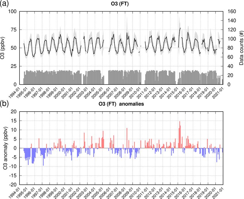
16238                   H. Clark et al.: The effect of the COVID-19 lockdowns on atmospheric composition at Frankfurt

   Many studies have focused on primary pollutants such as        tion in the Troposphere) satellite and noted that the CO lev-
NO2 , decreases of which were almost immediately apparent         els were lower during the first phase of the lockdown over
in satellite imagery from the TROPOspheric Monitoring In-         India but higher during the second phase. This was proba-
strument (TROPOMI) on the Sentinel-5 Precursor satellite          bly indicative of the longer lifetime of CO in the atmosphere
(Veefkind et al., 2012) over China in January–February (Liu       and the long-range transport of CO from a variety of global
et al., 2020) and later over Europe (Bauwens et al., 2020).       sources. Overall, the reductions in NO2 and CO in near-
Emissions of NO2 are strongly linked to economic activity         surface air masses due to COVID-19 lockdown conditions
(Duncan et al., 2016). Instruments such as TROPOMI have           range from 20 % to 80 % for NO2 and 20 % to 50 % for CO,
registered weekly cycles of NO2 and drops in NO2 related          for all observations reported globally (Gkatzelis et al., 2021).
to behavioural patterns of work and holiday periods (Beirle          The effects on the secondary pollutant ozone are more
et al., 2003; Tan et al., 2009). Thus, the large reductions       complex due to its chemistry. Tropospheric ozone is pro-
in NO2 in the tropospheric column during lockdown over            duced by the photochemical oxidation of methane, car-
the most economically active areas of Europe (in particular       bon monoxide and non-methane volatile organic compounds
the Po Valley, Italy) were quickly associated with the drop       (NMVOCs) in the presence of nitrogen oxides (NOx = NO+
in industrial output and emissions from transport. Reduc-         NO2 ). There is also a contribution from stratosphere-to-
tions of between 20 % and 38 % compared with the same             troposphere transport (Holton et al., 1995) in certain synoptic
periods in previous years were recorded (Bauwens et al.,          situations (Stohl et al., 2005; Gettelman et al., 2011; Akri-
2020). However, TROPOMI is a young instrument, launched           tidis et al., 2018). Near the surface, ozone is lost through
in October 2017, and as such, there is not a robust clima-        dry deposition, titration by NO and reactions with hydro-
tology with which to compare these changes during lock-           gen oxide radicals (HOx ) (Monks, 2005). The fall in ozone
down and in particular to control for the influence of dif-       precursors such as CO during lockdown, together with a de-
ferent meteorological conditions (e.g. Goldberg et al., 2020).    crease in available quantities of the NOx catalyst, might have
Relevant weather conditions might include higher planetary        been expected to lead to a fall in ozone. However, Y. Wang
boundary layer heights which drive down the surface con-          et al. (2020) found that over China, O3 increased, possibly
centrations of pollutants irrespective of any changes in emis-    because a lower atmospheric loading of fine particles led to
sions; windy periods, with their impact on the dispersion         less scavenging of HO2 and greater O3 production as a re-
and deposition of NO2 ; and cloudy skies with their impact        sult. Such effects have been noted over China during the
on satellite retrievals. As TROPOMI is sensitive to clouds,       summers of 2005–2016 (W. Wang et al., 2020) and so are
using only cloud-free columns can lead to a negative sam-         not unique to the lockdown period. Shi and Brasseur (2020)
pling bias. In many parts of Europe, skies were unusually         also found that ozone increased by a factor of 2 over north-
clear (van Heerwaarden et al., 2021; https://surfobs.climate.     ern China specifically noting the wintertime conditions dur-
copernicus.eu/stateoftheclimate/march2020.php, last access:       ing lockdown. Over southern Europe, ozone was also seen to
3 November 2021) due to the persistence of anticyclonic           increase up to 27 % in some places, explained by the reduc-
conditions and strongly reduced air traffic (Schumann et al.,     tion in NOx and lower titration by NO (Sicard et al., 2020).
2021b, a), and a negative bias may have been reinforced dur-      Ordóñez et al. (2020) cautioned that whilst NO2 fell across
ing the lockdown period (e.g. Barré et al., 2021; Schiermeier,    the whole European continent, the ozone anomalies were not
2020; , last access: 3 November 2021).                            always of the same sign. Ozone decreased over Spain but
   Drops in primary pollutants were also evident from             increased over much of northwestern Europe where mete-
ground-based air quality networks across Chinese and Eu-          orological conditions were favourable for ozone formation,
ropean cities; see the review by Gkatzelis et al. (2021) for      including elevated temperatures, low specific humidity and
a comprehensive overview. In Spain’s two largest cities,          enhanced solar radiation.
where lockdowns were extremely strict, the reductions in             A similar picture is drawn from the collection of data
NO2 concentrations were 62 % and 50 % (Baldasano, 2020).          from worldwide near-surface observations as reported by
Lee et al. (2020) calculated an average reduction in NO2 of       Gkatzelis et al. (2021). The fractional changes for ozone
42 % across 126 sites in the UK, with a 48 % reduction at         range from a decrease of 20 % in Central Asia (4 studies)
sites close to the roadside due to the drop in traffic emis-      to an increase of up to 20 % for several parts of the world
sions. Y. Wang et al. (2020) looked at six different pollutants   (Africa with 2 studies, South America with 17 studies, west-
(PM2.5 , PM10 , CO, SO2 , NO2 and O3 ) and found large reduc-     ern Asia with 17 studies and Southeast Asia with 19 studies).
tions in NO2 from traffic sources and a smaller reduction in      For Europe (134 studies), percentage changes in ozone are
CO from reduced industrial activities in northern China. Sim-     on average close to zero with few reported reductions of less
ilarly, Shi and Brasseur (2020) also noted a drop in CO across    than 20 % and increases of up to 65 %. Although most of the
the monitoring stations in northern China operated by the         reported datasets include the consideration of meteorological
China National Environmental Monitoring Center. Pathakoti         conditions, this variability highlights the dominant role of the
et al. (2021) looked at CO from TROPOMI compared with             meteorological situation in creating these ozone anomalies at
the climatology from the MOPITT (Measurements of Pollu-           the surface.

Atmos. Chem. Phys., 21, 16237–16256, 2021                                         https://doi.org/10.5194/acp-21-16237-2021
H. Clark et al.: The effect of the COVID-19 lockdowns on atmospheric composition at Frankfurt                              16239

   Fewer discussions have considered the free troposphere,        particles, and meteorological parameters including temper-
where measurements would be indicative of global or back-         ature and winds. A full description of the instruments that
ground changes in the levels of pollutants. Steinbrecht et al.    measure ozone and CO used here can be found in (Nédélec
(2021) looked at free-tropospheric ozone across the Northern      et al., 2015). The ozone instrument, a dual-beam ultraviolet
Hemisphere from balloon-borne ozonesonde measurements             absorption monitor, has a response time of 4 s and an accu-
from 1–8 km in altitude. They found a reduction in free-          racy estimated at about 2 ppbv (Thouret et al., 1998). This
tropospheric ozone of about 7 % compared with the 2000–           4 s response time corresponds to a vertical distance of about
2020 climatological mean which they largely attributed to         30 m. In the horizontal, the aircraft covers a distance of about
the reduction in emissions during the COVID-19 lockdowns.         80 km during the first 5 km of ascent (Petetin et al., 2018a).
   The IAGOS (In-service Aircraft for a Global Observing          Therefore during the ascent and descent phases of the flight,
System) instruments carried on commercial aircraft measure        IAGOS provides fine-scale quasi-vertical profiles. Carbon
the primary pollutant carbon monoxide and the secondary           monoxide is measured with an infrared analyser with a time
pollutant ozone, along with water vapour, clouds, and me-         resolution of 30 s (7.5 km at cruise speed of 900 km h−1 ) and
teorological parameters such as temperature and winds (Pet-       a precision estimated at 5 ppbv (Nedelec et al., 2003).
zold et al., 2015; Nédélec et al., 2015). Ninety percent of          IAGOS began in 1994 under the name MOZAIC (Mea-
the data are acquired in the upper troposphere–lower strato-      surement of Ozone and Water Vapour by Airbus In-service
sphere (UTLS) when the aircraft attain cruise altitude some-      Aircraft) (Marenco et al., 1998), and as such IAGOS has pro-
where between 300 and 180 hPa (9 to 12 km above mean              vided a long time series of ozone data over 27 (1994–present)
sea level). The remaining 10 % of data are collected dur-         years and of CO for almost 20 years (2001–present). The ho-
ing landing and take-off over more than 300 airports around       mogeneity of the time series since 1994 has been demon-
the world. During the COVID-19 lockdowns in Europe, there         strated by (Blot et al., 2021), giving confidence that IAGOS
was a large fall in passenger numbers with a consequent im-       data can be used for a robust climatology and for the study
pact on the number of IAGOS aircraft flying and the amount        of long-term trends. As mentioned above, this gives IAGOS
of data collected. However, one of the Lufthansa aircraft was     some important advantages over more short-lived datasets
converted to carry cargo and operated throughout the lock-        such as those from satellites and allows us to put any anoma-
down period. The aircraft made regular flights from Frankfurt     lies into context within the same reference observations.
to Asia, carrying important medical supplies. Frankfurt Air-         For the IAGOS measurements, a number of auxiliary di-
port has the longest, densest and most homogeneous time se-       agnostic fields are delivered with the data as standard level
ries of all the airports visited by IAGOS. Thus, the climatol-    4 products. These include potential vorticity, geopotential
ogy calculated there is the most robust (Petetin et al., 2016b)   height and boundary layer height which we will use in this
with ozone having been measured since 1994 and CO since           article. The boundary layer height which is defined as the
the end of 2001.                                                  boundary layer thickness (zPBL) plus orography is calcu-
   In this article, we present the observed anomalies of both     lated by interpolating the European Centre for Medium-
ozone and CO seen over Frankfurt and benefit from the fine        Range Weather Forecast’s (ECMWF) operational boundary
30 m vertical resolution throughout the troposphere to dis-       layer heights to the position and time of the IAGOS aircraft.
tinguish the surface anomalies from the observations in the       The ECMWF fields were 1◦ horizontal resolution and 3 h
free troposphere. This offers a valuable check on satellite       time resolution with 60, 90 or 137 levels in the vertical de-
data and adds unique and valuable vertical information which      pending on the time period used (http://www.iagos-data.fr/
is not offered by surface sites. We judge the significance of     #L4Place:, last access: 3 November 2021).
the ozone anomalies against the 26-year climatology (1994–           In order to determine the geographical origin and source
2019) at Frankfurt, putting the observed anomalies in context     of the CO measured by IAGOS, a tool known as SOFT-IO
with other important events such as the heatwave in 2003.         (Sauvage et al., 2017a, b) has been developed, which uses
To complement the IAGOS data at Frankfurt we use IASI-            FLEXPART (FLEXible PARTicle dispersion model; Stohl
SOFRID (Software for a Fast Retrieval of Infrared Atmo-           et al., 2005; Forster et al., 2007) to link the IAGOS mea-
spheric Sounding Interferometer (IASI) Data) CO retrieval         surements with emissions databases via 20 d back trajec-
which gives an idea of the extent of any regional changes         tories. For the entire IAGOS flight track, SOFT-IO v1.0
over Europe.                                                      (Sauvage et al., 2017a, 2018) estimates the source region of
                                                                  the CO contribution from 14 different world regions of emis-
                                                                  sions from the Copernicus Global Fire Assimilation System
2   Data                                                          (GFAS) v1.2. The source regions are as defined by the Global
                                                                  Fire Emissions Database (GFED), although the emissions in-
The research infrastructure IAGOS is described in detail in       ventories are GFAS. It can also estimate the contributions
(Petzold et al., 2015). Using commercial aircraft as a plat-      from anthropogenic sources or wildfires. As for the auxil-
form, IAGOS instruments make routine measurements of              iary diagnostic fields mentioned above, the meteorological
ozone and carbon monoxide along with water vapour, cloud          data for FLEXPART come from the 1◦ by 1◦ ECMWF oper-

https://doi.org/10.5194/acp-21-16237-2021                                       Atmos. Chem. Phys., 21, 16237–16256, 2021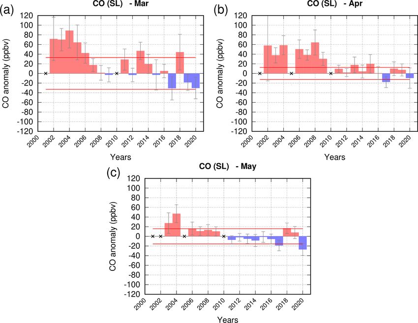
16240                   H. Clark et al.: The effect of the COVID-19 lockdowns on atmospheric composition at Frankfurt

ational analyses and forecasts with a 6 and 3 h time resolution
respectively (Sauvage et al., 2017b).
   To set the IAGOS measurements at Frankfurt Airport into
a regional context, we use CO satellite retrievals from the In-
frared Atmospheric Sounding Interferometer (IASI) on the
MetOp (Meteorological Operational satellite) meteorologi-
cal platforms (Clerbaux et al., 2009). These retrievals are
performed with the Software for a Fast Retrieval of IASI
Data (SOFRID) described in Barret et al. (2011); De Wachter
et al. (2012). This software is based on the RTTOV (Ra-
diative Transfer for Television Infrared Observation Satel-
lite (TIROS) Operational Vertical Sounder) operational ra-
diative transfer code (Saunders et al., 1999; Matricardi et al.,
2004) combined with the 1D-Var (one-dimensional varia-
tional analysis) software (Pavelin et al., 2008). For CO, the
SOFRID retrievals provide a maximum of two pieces of
information about the vertical profiles from the surface to
the lower stratosphere with a maximum sensitivity at about
800 hPa and an estimated error of about 10 % (De Wachter
et al., 2012).

3   Anomalies of ozone in spring 2020                              Figure 1. IAGOS observations of ozone for March and May 2020
                                                                   in black. The blue line is the average profile for March and May
In this first section, we look at the anomalies of ozone which     calculated over the reference time series (220 profiles) of the ozone
were strongly evident in spring 2020. Figure 1 shows the av-       observations for 2016–2019. The shaded area represents the inter-
                                                                   annual variability for March and May over the reference period.
eraged profile of ozone measured at Frankfurt for March and
                                                                   Horizontal lines denote the boundaries of the sections of study as
May 2020. There were no ozone data in April 2020, due to
                                                                   used in subsequent figures.
the ozone sensor being inoperative. The data were acquired
by an IAGOS-equipped Lufthansa passenger aircraft which
was based at Frankfurt. It was converted to cargo operations       per troposphere. In the period of MAM (March–April–May)
and was kept flying throughout the lockdown period, making         2020, there were notable departures from the climatology.
a total of 84 flights in March and May 2020.                       Ozone mixing ratios reached on average 42 ppbv in a layer
   In Fig. 1, the IAGOS observations are marked by the black       from the surface up to an altitude of 1000 m. Such values
solid line. The blue solid line represents the average for the     are more commonly found during summer heatwaves. In the
reference time series of 2016–2019, and the blue shaded en-        free troposphere from 2000–5000 m, the abundance of ozone
velope shows the interannual variability of March and May          is lower than normal, lying outside the expected interannual
over this period. We used a short and recent section of the        range. We consider some possible reasons for these anoma-
time series of ozone to account for any recent changes in          lies, in particular the possible link with the COVID-19 lock-
background amounts of ozone. Petetin et al. (2016b) found          downs, in the following sections.
only a weakly significant trend in ozone at Frankfurt in the
lower troposphere over the period of 1994–2012. Gaudel             3.1   Anomalies of ozone in the surface layer (> 950 hPa)
et al. (2020) considered the free troposphere from 700 to
250 hPa and the period of 1994–2016 and found small in-            The period of MAM 2020 corresponded to the period with
creases in ozone over Europe, and Cooper et al. (2020) found       the most stringent COVID-19 lockdowns across western Eu-
increases in the free troposphere over Europe based on the         rope, but each country had its own date of onset, dura-
years 1994–2017. Because of the considerable variability in        tion and level of severity. Measures of European mobility
the magnitude of trends over time, altitude and season, we         (Grange et al., 2021, based on Google mobility data) reveal
compare our results to a recent reference period of 2016–          that the depths of lockdown were in early April, showing a
2019.                                                              very slight recovery throughout May. At Frankfurt Airport,
   The profiles presented in Fig. 1 are similar to those pre-      there was 50 % less air traffic in March 2020 compared with
sented in Petetin et al. (2016b) based on the period of            March 2019, with nearly 80 % less air traffic in April and
1994–2012. They show the maximum ozone mixing ratios               May (according to Frankfurt Airport, FRAPORT, at https:
in the free troposphere to be about 60 ppbv, increasing from       //www.fraport.com/en/investors/traffic-figures.html, last ac-
21 ppbv at the ground and then increasing again in the up-         cess: 18 December 2020). This reduction was driven by a

Atmos. Chem. Phys., 21, 16237–16256, 2021                                           https://doi.org/10.5194/acp-21-16237-2021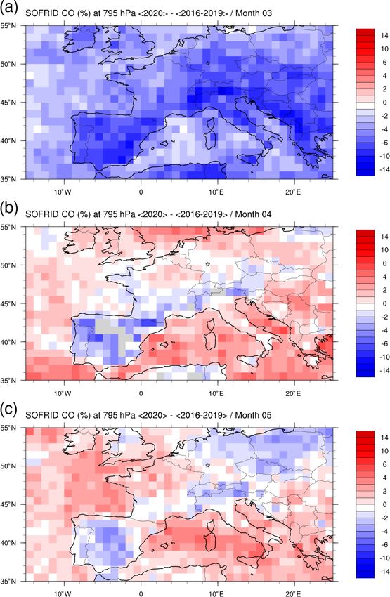
H. Clark et al.: The effect of the COVID-19 lockdowns on atmospheric composition at Frankfurt                              16241

fall in passenger numbers as lockdown measures increased          or lower boundary layer heights which trap the pollutants
around the world. According to Grange et al. (2021), the re-      near the surface. Otherwise, there can be a decrease in the
striction measures began in Germany on 22 March 2020 and          sinks of ozone, such as a decrease in the rate of dry depo-
had a “stringency index”, defined as “a measure of the strict-    sition or a decrease in titration by NO due to a reduction in
ness of ‘lockdown style’ policies”, that remained relatively      the emissions of NOx . During the 2003 heatwave, IAGOS
high until the end of May, but the lockdown was by no means       data showed that there were positive anomalies at Frankfurt
the strictest in Europe.                                          in both ozone and the precursor carbon monoxide in the low
   In Fig. 2, we present the anomalies in ozone for the in-       troposphere, with the ozone anomalies up to 2.5 km deep and
dividual months of March and May 2020. As mentioned               with the magnitude of the anomalies increasing towards the
above, we did not have any ozone data in April 2020. We re-       surface (Tressol et al., 2008). Tressol et al. (2008) found that
quire there to be 7 d to make the monthly average; otherwise      near the surface, ozone was almost twice the normal amount,
the month is excluded. Excluded months are marked with a          and CO was more than 20 % higher. The increased CO was
cross. During the lockdown period, there were fewer flights       due to the transport of plumes from wildfires over Portugal
than normal, and we need to be aware of any sampling bias         exacerbated by the dry conditions created by the heatwave.
that this may introduce. The number of profiles per month         Thus, during the 2003 heatwave, the increased ozone was
is shown as the solid grey bars in top panel of Fig. 3. The       caused by an increase in precursors and the favourable mete-
confidence limits, shown in Fig. 2, account for the differing     orological conditions.
number of profiles per month. The confidence limits are cal-         During lockdown, the chemical environment was quite
culated using Student’s t distribution.                           different. The positive anomaly of ozone was accompa-
   It was during the month of May, after the lockdown had         nied by a drop in the amount of NO as evidenced by the
been in place for several weeks, that the ozone anomaly in the    TROPOMI satellite measurements of NO2 (Bauwens et al.,
surface layer (pressure P > 950 hPa) was most pronounced          2020), and there is some evidence from IAGOS measure-
(Fig. 2). In May, ozone was recorded at +11.9 ppbv (+32 %)        ments that levels of the precursor carbon monoxide also fell
higher than the reference average (2016–2019) and was the         (see Sect. 4). The anomaly of ozone in the surface layer
largest anomaly for the month of May since the time series        (extending to 1 km; cf. 2.5 km in the 2003 heatwave) was
began in 1994. The magnitude of the anomaly including the         most likely due to the combination of increased production
95 % confidence limits is outside the interannual variability,    of ozone due to the exceptionally sunny conditions across
based on the reference years, given by the solid blue line. The   a large sector of northern Europe (van Heerwaarden et al.,
anomaly is apparent in the first 1000 m of the atmosphere         2021; Ordóñez et al., 2020; see also https://surfobs.climate.
(Fig. 1). A positive anomaly was also observed in March           copernicus.eu/stateoftheclimate/may2020.php, last access:
2020 (5 %) with a smaller value compared with May. Posi-          3 November 2021) along with the removal of one of the
tive anomalies in ozone have not been unusual in recent years     ozone sinks, particularly the reduction in ozone titration be-
(see Fig. 3), suggesting that the lockdowns are not the only      cause of the reduction in NO. In addition, the stable meteoro-
explanation.                                                      logical conditions, lack of wind and air stagnating over towns
   To set the magnitude of these anomalies into context with      could also have contributed to the accumulation of pollutants
other periods, the time series for each month for the sur-        and of ozone itself in the boundary layer. Some recent studies
face layer over Frankfurt is shown in the bottom panel of         have attempted to tease out the contribution of meteorology
Fig. 3. The anomalies are calculated with respect to 2016–        from the impact of the changes in the emissions of precursors
2019. There were a few occasions when the ozone anoma-            (Ordóñez et al., 2020; Petetin et al., 2020; Lee et al., 2020).
lies were comparable to that of May 2020 including a peak         All found that there were important and differing impacts of
of similar magnitude in February 2005. In the other seasons,      meteorology but that there were changes in NOx that were
the peaks were August 2015 and September 2016 when there          unattributed to the meteorological conditions and linked to
were short heatwaves and the well-known heatwave in Au-           falling emissions during the lockdowns.
gust 2003 which we discuss here, as it was well documented           The magnitude of any anomaly may be significantly influ-
with IAGOS data (Tressol et al., 2008; Ordóñez et al., 2010).     enced by the sampling times within the diurnal cycle. Petetin
It should be noted that, when compared with the recent refer-     et al. (2016a) described the typical diurnal cycle of ozone
ence period of 2016–2019, the magnitude of the anomaly in         at Frankfurt Airport observed with IAGOS data at different
August 2003 is diminished, suggesting that these high ozone       altitudes. They noted that the mixing ratios of ozone are at
abundances have become less unusual.                              their minimum at nighttime due to dry deposition and titra-
   An increase in ozone near the surface can result from          tion by NO in the shallow nocturnal boundary layer and
increased production of ozone or reduced sinks of ozone,          reach a maximum in the afternoon, due to photochemistry
depending on the conditions and the time of day. Positive         and mixing with ozone-rich layers above the boundary layer.
anomalies of ozone may be due to an increase in the precur-       Petetin et al. (2016a) showed the diurnal cycle of ozone at
sors of ozone or a prevalence of certain meteorological con-      Frankfurt to be maximum between 12:00 and 18:00 UTC in
ditions including increased UV radiation, stagnant air masses     MAM in the layers below 900 hPa. The amplitude is at its

https://doi.org/10.5194/acp-21-16237-2021                                       Atmos. Chem. Phys., 21, 16237–16256, 2021
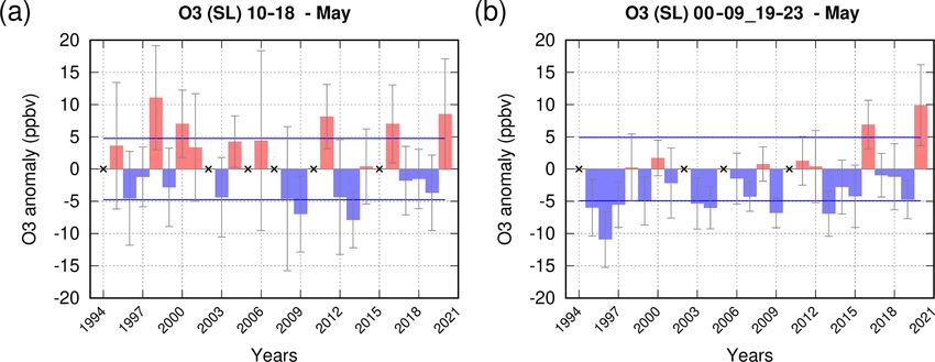
16242                    H. Clark et al.: The effect of the COVID-19 lockdowns on atmospheric composition at Frankfurt

Figure 2. Anomalies of ozone for 1994–2020 calculated with respect to 2016–2019 for the months of (a) March and (b) May for the surface
layer (> 950 hPa; SL). There were no ozone data in April 2020. The grey bars represent the 95 % confidence limits, and the blue horizonal
lines represent the interannual variability.

Figure 3. Monthly time series for 1994–2020 of O3 for the surface layer over Frankfurt (a). The grey bars represent the number of daily
profiles used to calculate the monthly means shown in black. Grey shading represents the standard deviation for each month. (b) The monthly
anomalies calculated with respect to the reference average of 2016–2019 in the surface layer. Please note that the date format used in this
figure is yyyy-mm.

maximum at the surface and decreases with altitude, becom-              in 2020 compared with the same months in the reference pe-
ing almost insignificant at altitudes above 900 hPa. We con-            riod of 2016–2019. In the climatology, there is a bias towards
sider the anomaly observed in May with respect to the di-               measurements in early morning. In March 2020, the distribu-
urnal cycle of ozone. More measurements in the afternoon                tion is similar to that during the reference period, but in May
would lead to an oversampling of the maximum and a pos-                 2020 there is a bias towards measurements in early afternoon.
itive ozone anomaly, and conversely, more measurements at               This reflects the different flight operations carried out during
nighttime would be an oversampling of the minimum and a                 the COVID-19 period.
negative anomaly. In Fig. 4, we can see the hourly distribu-               To account for this bias, we calculate the anomaly for
tion of the IAGOS profiles for the months of March and May              May for the hours when the diurnal cycle is at its maximum

Atmos. Chem. Phys., 21, 16237–16256, 2021                                                https://doi.org/10.5194/acp-21-16237-2021

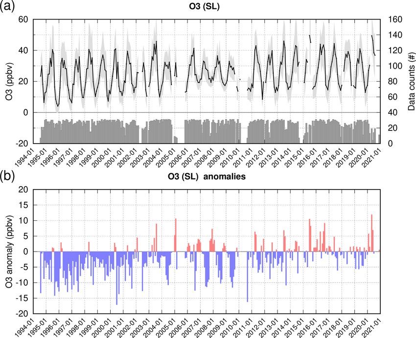
H. Clark et al.: The effect of the COVID-19 lockdowns on atmospheric composition at Frankfurt                                  16243

Figure 4. Number of profiles by hour of the day (UTC) for (a) March 2020 and (b) May 2020 (counts on left-hand axis) compared with the
same months in the reference period of 2016–2019 (counts on right-hand axis).

Figure 5. Anomalies of ozone for 1994–2020 for the month of May in the surface layer (> 950 hPa) for the (a) daytime (10:00–18:59 UTC)
and (b) nighttime (00:00–09:59 and 19:00–23:59 UTC). The grey bars represent the 95 % confidence limits, and the blue horizonal lines
represent the interannual variability.

(10:00–18:59 UTC) and the hours when the diurnal cycle is            was short-lived. We now explore the vertical extent of the
at its minimum (00:00–09:59 and 19:00–23:59 UTC), apply-             ozone anomaly, using the unique perspective that IAGOS of-
ing this to both the climatology and 2020 (Fig. 5). This is          fers.
based on the diurnal cycle for ozone at Frankfurt in MAM de-
scribed in Petetin et al. (2016a) and depends upon ozone pho-        3.2   Anomalies of ozone in the free troposphere
tochemistry and the dynamical development of the bound-                    (850–350 hPa)
ary layer. In Fig. 5a there remains a significant increase in
ozone in May during the day (8.3 ppbv, 19 %), comparable             In contrast to the positive anomaly in the surface layer up to
with other anomalies which have occurred four times dur-             1000 m, the anomaly in the free troposphere above 2000 m is
ing the last 26 years. This likely reflects the meteorological       negative (Fig. 1), lying just outside of the range of interan-
conditions that were relatively exceptional and favourable to        nual variability based on the 26-year time series shown in
ozone formation. In Fig. 5b the nighttime increase (9.9 ppbv,        Fig. 6. The grey bars in the top panel of Fig. 6 represent
29 %) is clearly the most significant observed in the time se-       the number of available daily profiles in each month (where
ries. We infer that the positive anomaly in ozone at nighttime       there was more than 7 d available in the month). There was a
is linked to the drop in NO2 at Frankfurt (Barré et al., 2021)       −7.6 ppbv or −14 % change in ozone in March (Fig. 7). This
during lockdown and the consequent reduction in ozone titra-         negative anomaly is the largest for March since 1997 for the
tion. Once meteorological changes were accounted for, the            IAGOS observations in the free troposphere. It is too early
estimates of lockdown-induced NO2 changes for Frankfurt              to have resulted from the European lockdowns and not easy
were −24 % and −33 % based on TROPOMI observations                   to link to the Asian lockdowns. There was only a −3.4 ppbv
and surface stations respectively (Barré et al., 2021). The          (−5 %) change in ozone in the free troposphere over Frank-
positive ozone anomaly observed in IAGOS data for the sur-           furt in May 2020 which might be linked to regional Euro-
face layer is in agreement with the other studies cited based        pean lockdowns (Fig. 7) but is not outside the interannual
on the surface networks and as reviewed by (Gkatzelis et al.,        variability. We had no data for April 2020. The IAGOS data
2021). The IAGOS data for the remainder of 2020 (Fig. 3)             show that ozone levels remained lower than usual for sev-
show smaller positive anomalies which were not significant           eral months after the main lockdown period ended, with a
within the time series, suggesting that the anomaly in MAM           −10 % anomaly being observed in July (the largest anomaly

https://doi.org/10.5194/acp-21-16237-2021                                           Atmos. Chem. Phys., 21, 16237–16256, 2021
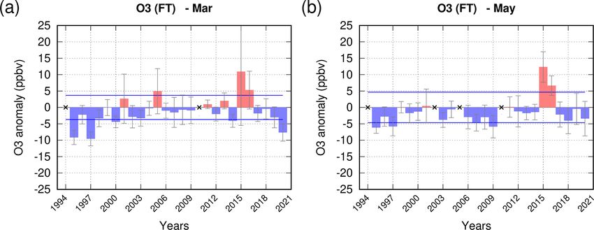
16244                    H. Clark et al.: The effect of the COVID-19 lockdowns on atmospheric composition at Frankfurt

Figure 6. Monthly time series for 1994–2020 of O3 for the free troposphere (850–350 hPa; FT) over Frankfurt (a). The grey bars represent
the number of daily profiles used to calculate the monthly means shown in black. Grey shading represents the standard deviation for each
month. (b) The monthly anomalies calculated with respect to the reference average of 2016–2019 in the free troposphere. Please note that
the date format used in this figure is yyyy-mm.

Figure 7. Anomalies of ozone for 1994–2020 for the months of (a) March and (b) May in the free troposphere (850–350 hPa). There were
no ozone data in April 2020. The grey bars represent the 95 % confidence limits, and the blue horizonal lines represent the interannual
variability.

recorded for July in the 27-year time series; see Fig. A1) as         dances fell widely during MAM due to the combined effect
the economic recovery and emissions remained suppressed               of the lockdown measures across Europe, but evidence from
throughout summer 2020 (Fig. 6). Over the period of April–            the ozonesondes (Steinbrecht et al., 2021) suggests that we
August 2020, a 7 % drop was seen by ozonesondes (Stein-               can expect a degree of geographical variability. For example,
brecht et al., 2021) from 1–8 km in altitude. This figure rep-        there was no notable decrease in free-tropospheric ozone in
resents a mean value across all sites in the Northern Hemi-           the sparsely sampled Southern Hemisphere.
sphere over the period of April–August 2020 compared with
the 2000–2020 climatology. The negative anomaly seen at
Frankfurt in IAGOS data may illustrate that ozone abun-

Atmos. Chem. Phys., 21, 16237–16256, 2021                                              https://doi.org/10.5194/acp-21-16237-2021
H. Clark et al.: The effect of the COVID-19 lockdowns on atmospheric composition at Frankfurt                                  16245

4     Carbon monoxide in spring 2020

As mentioned in the Introduction, some studies have demon-
strated a fall in the ozone precursors during MAM 2020. The
reductions in CO in near-surface air masses due to COVID-
19 reported by (Gkatzelis et al., 2021) ranged from 20 % to
50 % for CO. Due to the long (weeks to months) lifetime of
CO in the atmosphere, the causes of these decreases in CO
are difficult to attribute. Figure 8 shows the seasonally aver-
aged profile of CO measured at Frankfurt for MAM 2020,
with the black solid line denoting the IAGOS observations.
The red solid line represents the seasonal average for the ref-
erence period of 2016–2019, and the red shaded area shows
the interannual variability of MAM over the reference period.
Often, there are fewer IAGOS observations near the surface
than in the free troposphere, which leads to the standard de-
viation being greater near the surface as shown by the wider
envelope (shaded red area). The inflection of the black curve
results from a small number of flights which nevertheless
fall within the expected range shown by the red shaded area.
Despite the length of the time series being nearly 20 years,
we have chosen the same short segment (2016–2019) for
our reference period as we used for ozone. This is because         Figure 8. IAGOS observations of CO for March–April–May
there is a negative trend in CO (−1.9 % yr−1 and 2.0 % yr−1        (MAM) 2020 in black. In red, the average profile for MAM cal-
from Petetin et al. (2016b) for lower-troposphere and mid-         culated over the reference period of 2016–2019 (300 profiles). The
troposphere springtime respectively), and thus all recent data     shaded area represents the interannual variability for MAM over
show a negative anomaly (see also Fig. 9). We return to this       this reference period. Horizontal lines denote the boundaries of the
                                                                   sections of study as used in subsequent figures.
point later. For the period of MAM 2020 we can see that the
CO mixing ratios are below the average for recent years (red
line) and lie at the lower limit given by the envelope of inter-
annual variability.                                                only months where there is at least 7 d are used to make
   Similar averaged profiles were presented in Petetin et al.      the monthly average; otherwise the month is excluded. The
(2016b) based on the period (2002–2012) where the aver-            anomalies in Fig. 9 are calculated with respect to the short
age mixing ratio at 2000 m for MAM was 150 ppbv. For our           reference time series of 2016–2019. In 2020, we can see a
segment of 2016–2019 the average mixing ratio for MAM              drop in CO mixing ratios with the lowest values in the time
at 2000 m was 140 ppbv, indicative of the negative trend of        series being recorded in February 2020.
CO. Over the period of 2002–2020, there has been a drop               Figure 10 shows the anomalies for March, April and May
in CO mixing ratios observed at Frankfurt due to a reduc-          for 2001–2020. In May, towards the end of the lockdown pe-
tion in emissions and the impact of emissions protocols.           riod, the anomaly was (−27.2 ppbv, −15 %), and the 95 %
However, there is a strong interannual variability in the free-    confidence limit is outside the range of interannual variabil-
tropospheric background which reflects the interannual vari-       ity. However, inspection of the time series (Fig. 9) reveals
ability in global biomass burning, anthropogenic emissions,        that the greatest anomaly relative to 2016–2019 was actually
and the complex interactions with other species such as OH         apparent in February, before the European lockdown mea-
and O3 . The background abundance of CO therefore depends          sures began. When compared with the reference time se-
on the selected segment of the time series.                        ries (2016–2019), the anomaly in February was (−61.4 ppbv,
                                                                   −26 %; see Appendix Fig. B1). February lies outside our
4.1    Anomalies of carbon monoxide in the surface layer           main period of interest, but the large anomaly observed then
       (> 950 hPa)                                                 suggests that the drop in CO at the surface observed in subse-
                                                                   quent months is not wholly attributed to the drop in emissions
In the surface layer, we see a downward trend in monthly           linked to lockdown. Indeed, a fall in NO2 levels was also
values of CO on the seasonal and annual scale (see Fig. 9) in      reported by Peuch (2020) from February onwards. Peuch
agreement with Petetin et al. (2016b). Also shown in Fig. 9 is     (2020) suggested that the driver of this could be an increase
the number of flights per month as the solid grey bars which       in boundary layer heights and consequent dilution of the pol-
reveals a reduction in flights due to the reduction in global      lutants near the surface. To investigate if this could be a factor
travel during the first phase of the pandemic. As with ozone,      in the low CO seen in IAGOS data, we examine the boundary

https://doi.org/10.5194/acp-21-16237-2021                                         Atmos. Chem. Phys., 21, 16237–16256, 2021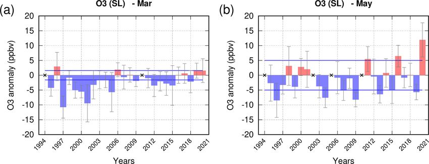
16246                    H. Clark et al.: The effect of the COVID-19 lockdowns on atmospheric composition at Frankfurt

Figure 9. Monthly time series for 2001–2020 of CO for the surface layer over Frankfurt (a). The grey bars represent the number of daily
profiles used to calculate the monthly means shown in black. Grey shading represents the standard deviation for each month. (b) The monthly
anomalies calculated with respect to the reference average of 2016–2019 in the surface layer. Please note that the date format used in this
figure is yyyy-mm.

Figure 10. Anomalies of CO for 2001–2020 for the months of (a) March, (b) April and (c) May, in the surface layer (> 950 hPa). The grey
bars represent the 95 % confidence limits, and the blue horizonal lines represent the interannual variability.

Atmos. Chem. Phys., 21, 16237–16256, 2021                                                https://doi.org/10.5194/acp-21-16237-2021
H. Clark et al.: The effect of the COVID-19 lockdowns on atmospheric composition at Frankfurt                                  16247

layer heights for 2020 compared with the 2016–2019 aver-
age.
    We calculated the boundary layer height (the boundary
layer height (BLH) is the boundary layer thickness (zPBL)
plus orography) by interpolating the ECMWF operational
boundary layer heights to the position of the IAGOS aircraft.
The ECMWF fields had a 1◦ horizontal resolution and 3 h
time resolution. We used a bilinear interpolation in space us-
ing a distance weighting from the four nearest grid cells to
the IAGOS position and a linear interpolation in time. This
calculated BLH is one of a number of added-value prod-
ucts which are included with IAGOS data as a standard in
“level 4”. Due to the diurnal variability of the boundary layer
height as the convective boundary layer develops during the
day and the seasonal variability in the time of sunrise and       Figure 11. Monthly averaged boundary layer heights interpolated
sunset, Fig. 11 is divided into two time slots. The top panel     in space and time from the 3-hourly ECMWF operational fields on
shows the afternoon–evening, defined as 3 h after sunrise un-     1◦ resolution for afternoon–evening (a) and nighttime–morning (b).
til 2 h before sunset. The bottom panel shows the nighttime–      Afternoon–evening is defined as 3 h after sunrise until 2 h before
                                                                  sunset, and nighttime–morning is defined as 2 h before sunset until
morning defined as 2 h before sunset until 3 h after sunrise.
                                                                  3 h after sunrise. The boundary layer heights are expressed as a per-
Each time series shows the percentage difference with re-
                                                                  centage difference from the mean height calculated over the period
spect to the monthly mean calculated for 2016–2019 and is         of 2016–2019.
shown for 8 months (January–August) for each year between
2016 and 2020. The depth of the nighttime boundary layer
increased by 60 % (400 m) in February and 70 % in May
with respect to the monthly mean from 2016–2019 and was
greater than any other anomaly observed over the period of
2016–2019. The anomaly covers the MAM period and may
partly explain the decreased concentrations of CO in the sur-
face layer. We accounted for these changes by integrating
the CO over the height of the boundary layer. A negative
anomaly of 30 ppbv in February and of 12 ppbv in March
and May was noted which can be ascribed to decreases in
emissions.
    The observations of CO near the surface from IAGOS are
                                                                  Figure 12. Emissions regions used for the SOFT-IO v1.0 model.
less impacted by the local emissions at airports than might be    BONA: Boreal North America; TENA: Temperate North Amer-
thought. Petetin et al. (2018a) compared IAGOS with moni-         ica; CEAM: Central America; NHSA: Northern Hemisphere
toring stations from the local air quality monitoring network     South America; SHSA: Southern Hemisphere South America;
(AQN) and more distant regional surface stations from the         EURO: Europe; MIDE: Middle East; NHAF: Northern Hemisphere
Global Atmospheric Watch (GAW) network. They found that           Africa; SHAF: Southern Hemisphere Africa; BOAS: Boreal Asia;
the mixing ratios of CO and O3 close to the surface do not        CEAS: Central Asia; SEAS: Southeast Asia; EQAS: Equatorial
appear to be strongly impacted by local emissions related         Asia; AUST: Australia and New Zealand.
to airport activities and are not significantly different from
those mixing ratios measured at surrounding urban back-
ground stations. It is therefore unlikely that the reduction in   older than 20 d or secondary CO produced by chemical re-
airport activity during COVID-19 was a big contributor to the     actions in situ. It is more adapted to look at well-defined
negative anomaly observed at Frankfurt in the surface layer.      plumes of pollution visible against the background. In addi-
In the free troposphere, the local emissions have even less ef-   tion, the anthropogenic emissions database (MACCity; Mon-
fect, and the mixing ratios tend to background concentrations     itoring Atmospheric Composition and Climate) has not been
as typically measured by the GAW regional stations.               updated to take account of the COVID-19 period. This makes
    To examine more closely the source regions of the CO          the relative contribution from each source difficult to deter-
at Frankfurt, we have used the SOFT-IO tool which rou-            mine. For these reasons we will focus on the geographic ori-
tinely connects emissions databases to each IAGOS mea-            gin of the CO at Frankfurt as determined by the trajectory
surement via FLEXPART trajectory calculations (Sauvage            calculations. The source regions are defined as in Fig. 12.
et al., 2017b, 2018). SOFT-IO does not calculate the back-        The trajectories terminate at the aircraft position within the
ground amounts of CO which include CO from emissions              surface layer. We compare the source regions in 2020 with

https://doi.org/10.5194/acp-21-16237-2021                                        Atmos. Chem. Phys., 21, 16237–16256, 2021
16248 H. Clark et al.: The effect of the COVID-19 lockdowns on atmospheric composition at Frankfurt
data over Frankfurt to the larger geographical context. Satel-
lite fields of CO in the tropospheric column are presented
for Europe in Fig. 15. Figure 15 represents the percentage
change in the tropospheric CO at 795 hPa with respect to the
2016–2019 average as retrieved from IASI for the months
of March, April and May. In March, the IASI-SOFRID data
confirm the negative anomaly in CO present at Frankfurt,
which is generalized over large parts of Europe. In April and
May, the IASI-SOFRID data showed little anomaly at Frank-
furt and a mixed picture over Europe. Thus, the IAGOS and
IASI data show some reduction in CO during the lockdown
period which is not unexpected given the trend towards de-
creased CO. It is difficult to link this anomaly to the lock-
down measures due to other factors such as the increased
Figure 13. Contribution from different source regions to the CO in
the surface layer at Frankfurt in MAM 2020 compared with MAM
boundary layer height, the long-range global transport of CO
2016–2019. The colours correspond to the regions in Fig. 12. and interannual variability.
Using the same trajectory analysis as for Fig. 13, Fig. 16
shows that in MAM 2020, there was a much lower amount
those in our reference period of 2016–2019. In Fig. 13, we of CO from sources in Europe than in MAM 2016–2019 and
show the source region of the emissions. In agreement with an increase in the contribution from North America (TENA)
Petetin et al. (2018b), our analysis shows that the largest con- and from Central Asia (CEAS). We suggest that the increase
tribution to CO measured at Frankfurt is from the European in air masses carrying CO from anthropogenic and biomass-
region. Usually in this period, the contribution from biomass- burning sources from outside Europe offset the effects of the
burning emissions to the surface CO is small. In 2020, there cut in emissions during the European lockdown resulting in a
was a smaller absolute contribution to the surface CO from smaller-than-anticipated negative anomaly observed by both
biomass-burning emissions (1.3 ppbv in 2020 compared with IAGOS and IASI-SOFRID. This result is similar to that of
2.7 ppbv in 2016–2019) with the relative contribution being Field et al. (2020), who noted only a 2 % change in back-
10 % in the reference period. Most of the emissions in Europe ground abundances of CO over eastern China despite the
in 2020 were therefore anthropogenic. The majority (70 %) cut in industrial emissions during the Chinese lockdown. In
of the CO at Frankfurt had a European origin in both 2020 the case of Field et al. (2020) it was the cross-border trans-
and in the reference period of 2016–2019. In 2020, there port from areas with active biomass burning that offset the
was a greater contribution from sources in North America drop in anthropogenic emissions. In our reference period,
(TENA and BONA) and Asia (CEAS) compared with 2016– the mean biomass-burning contributions to the anomaly were
2019, which reflects the interannual variability of different about 3 ppbv or 20 %, whereas in 2020, the contribution was
air masses arriving in Europe. This analysis shows that it is 2 ppbv. As the contribution from biomass burning is small in
primarily local emissions across Europe that are reflected in Europe in MAM, the main influence to the CO loading over
the CO recorded at Frankfurt in the surface layer, and there- Europe is from anthropogenic emissions from several source
fore we can suppose that the lockdown measures played a regions with more or less stringent lockdown measures.
significant role. In the free troposphere, which we discuss in In summary for this section on CO, we conclude that
the following section, we will see that inter-continental trans- the drop in surface CO is largely the result of the drop in
port has a more important contribution. emissions during European lockdown, with higher than usual
boundary layer heights further diluting the surface concentra-
4.2 Anomalies of carbon monoxide in the free tions. In the free troposphere, where the negative anomalies
troposphere (850–350 hPa) were not outside expected interannual variability, the influ-
ence of long-range transport is more apparent and offsets the
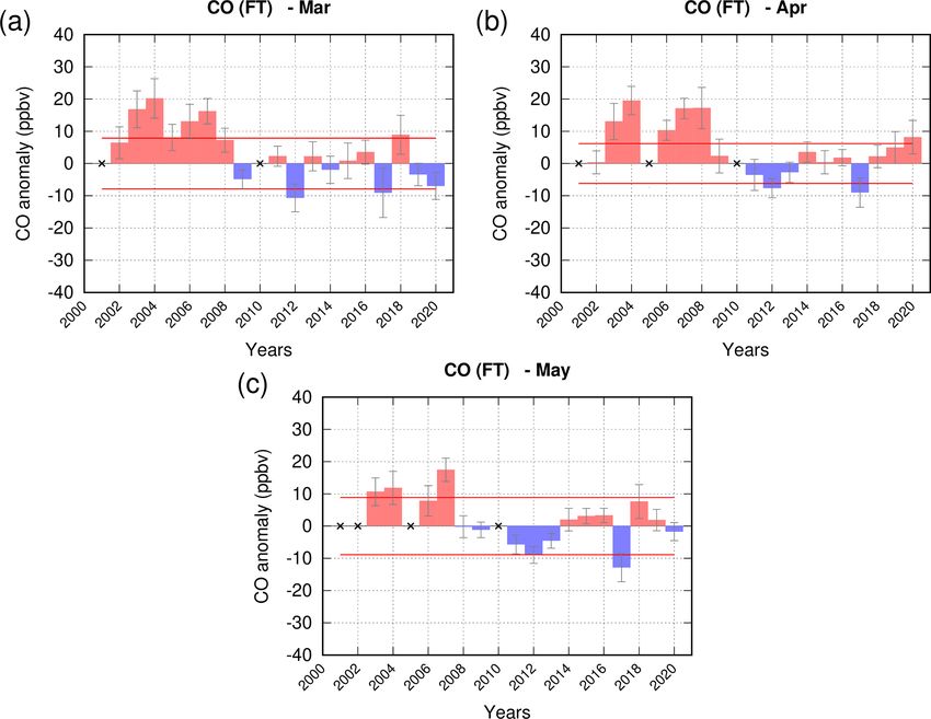
In the free troposphere, the anomalies of CO (Fig. 14) were impact of the reduction in CO emissions across Europe.
negative in March (−6.9 ppbv, −5 %) and May (−1.8 ppbv,
−1 %) but much smaller in magnitude than in the surface
layer (see Sect. 4.1) and do not exceed interannual variabil- 5 Conclusions
ity once the confidence limits have been considered. The
time series of CO in the free troposphere from 2001–2020 In this article, we use the IAGOS dataset of in situ observa-
is included for reference in Fig. B2. In April, the anomaly tions of ozone and carbon monoxide collected during landing
was positive (8.2 ppbv, 6 %). Since the free troposphere is and take-off at Frankfurt Airport. The atmosphere is sam-
more representative of the background concentrations due to pled from the surface to the upper troposphere, forming a
mixing and transport, it is instructive to relate the IAGOS quasi-vertical profile. The data form part of a time series
Atmos. Chem. Phys., 21, 16237–16256, 2021 https://doi.org/10.5194/acp-21-16237-2021H. Clark et al.: The effect of the COVID-19 lockdowns on atmospheric composition at Frankfurt 16249 Figure 14. Anomalies of CO for 2001–2020 for the months of (a) March, (b) April and (c) May, in the free troposphere (850–350 hPa). The grey bars represent the 95 % confidence limits, and the blue horizonal lines represent the interannual variability. which extends back for 27 years for ozone and 20 years for The magnitude of this anomaly is comparable to that dur- CO. We considered whether anomalies of ozone and CO at ing the European heatwave in August 2003 which was one of Frankfurt during MAM 2020 were related to changes in at- the most significant air quality events in Europe (e.g. Tres- mospheric composition resulting from the COVID-19 lock- sol et al., 2008). When compared with the recent reference downs, which reduced the industrial and traffic emissions of period of 2016–2019, the magnitude of the anomaly in Au- ozone precursors (e.g. Bauwens et al., 2020; Barré et al., gust 2003 is diminished, suggesting that these high ozone 2021). We compared MAM 2020 with a baseline period of abundances are no longer unusual. Although the anoma- 2016–2019 to account for recent increases in ozone and de- lies of ozone were of similar magnitude to those during the creases in CO. During MAM 2020, we noted a 19 % increase 2003 heatwave, the chemical environment during the lock- in ozone in the surface layer (> 950 hPa, 600 m). The month down period was quite different. During the 2003 heatwave, of May saw a significant anomaly (32 %), the largest since IAGOS data showed that there were positive anomalies at the time series began in 1994. Frankfurt in both ozone and the precursor carbon monoxide There was a large increase in ozone in the daytime in May in the low troposphere (Tressol et al., 2008). The increased 2020 (19 %), but the increase at nighttime (29 %) was even CO was due to the transport of plumes from wildfires over larger and has not been seen before in the 26-year time se- Portugal exacerbated by the dry conditions created by the ries. Despite the fall in the abundance of NOx over Europe heatwave. Thus, during the 2003 heatwave, the increased (as seen by satellite data), there were still enough available ozone caused the favourable meteorological conditions and precursors to produce ozone under the meteorological con- an increase in precursors, whereas during lockdown, the pos- ditions, especially enhanced solar radiation, that were very itive anomaly of ozone was accompanied by favourable me- favourable at the time (van Heerwaarden et al., 2021). The teorology and a fall in precursors. larger increase at nighttime, along with the observation that In the free troposphere, ozone abundances fell slightly. For NO2 fell by between 24 % and 33 % (Barré et al., 2021), sug- the period of MAM 2020 ozone was 10 % lower than the gests that less ozone was lost through titration with NO due mean of 2016–2019 based on the same months. The IAGOS to the reduction in the NO reservoir during the lockdown pe- time series shows that these free-tropospheric abundances of riod, signifying a reduction in one of the sinks of ozone. Fur- ozone were the lowest since 1997, which is probably more thermore, we noted an increase in the depth of the nighttime reflective of the widespread reduction of emissions over Eu- boundary layer, which would be expected to further reduce rope and beyond, with less of an impact from local meteorol- the sinks of ozone through less titration and deposition. ogy and chemistry. The results from IAGOS are also consis- https://doi.org/10.5194/acp-21-16237-2021 Atmos. Chem. Phys., 21, 16237–16256, 2021
16250                   H. Clark et al.: The effect of the COVID-19 lockdowns on atmospheric composition at Frankfurt

                                                                    Figure 16. Contribution from different source regions to the CO
                                                                    in the free troposphere at Frankfurt in MAM 2020 compared with
                                                                    MAM 2016–2019. The colours correspond to the regions in Fig. 12.

                                                                       In the free troposphere there is a small reduction in CO
                                                                    in March (−6.9 ppbv, −5 %) and May (−1.8 ppbv, −1 %)
                                                                    which is smaller than at the surface over Frankfurt and
                                                                    remains within the range of interannual variability. IASI-
                                                                    SOFRID fields of CO show a clear decrease in CO during
                                                                    March over all of Europe. In April and May small positive
                                                                    and negative anomalies over northern Europe and mostly
                                                                    negative anomalies over the Iberian Peninsula are detected
                                                                    by IASI-SOFRID. In the free troposphere, there is an impor-
                                                                    tant role of transport of CO from distant biomass and an-
                                                                    thropogenic sources. In particular in MAM 2020, there was
                                                                    a greater contribution from CO originating in North America
                                                                    and Asia. The contribution by air masses from outside Eu-
Figure 15. Percentage change of IASI-SOFRID carbon monoxide         rope may have offset some of the drop in CO resulting from
at 795 hPa in (a) March, (b) April and (c) May 2020 compared with   the reduction in regional European emissions, with the result
the reference average period of 2016–2019.                          that the lockdown measures did not have a big impact on CO
                                                                    in the free troposphere.
                                                                       The lockdowns provided a unique experiment to assess
tent with those from the balloon-borne ozonesondes reported         the impact of a reduction of economic activities on atmo-
by Steinbrecht et al. (2021), who noted a 7 % drop in tropo-        spheric composition and climate. The IAGOS data comple-
spheric ozone compared with the 2000–2020 climatological            ment other in situ data from the ozonesonde network, with
mean. They also attributed this to the reduction in pollution       the added value of having ozone precursors measured simul-
during the COVID-19 lockdowns.                                      taneously. This study demonstrates the importance of long
   A reduction in CO was seen at Frankfurt, with an 11 % re-        and continuous time series in setting this brief period in con-
duction found in the surface layer but no anomaly in the free       text, since there are many competing factors, and it is difficult
troposphere as averaged over MAM. The attribution of this           to attribute a single cause. We have considered various me-
decrease to the drop in emissions during lockdown is compli-        teorological factors for both ozone and CO near the surface
cated by the fact that the boundary layer heights were anoma-       and for interannual variability and long-range transport in the
lously high during this period and might therefore have con-        free troposphere. We look forward to future model sensitivity
tributed to a dilution of the CO at the surface. However,           studies to separate these factors and to provide a more realis-
the negative anomalies persist despite controlling for this. It     tic magnitude of the impact of lockdown on the environment.
should be noted that the greatest decrease in CO occurred in
February (26 %), before lockdown measures had been intro-
duced in Europe. Our trajectory analysis shows that the CO
is largely of European origin, and therefore we suggest the
impact of the lockdown on abundances of CO is likely.

Atmos. Chem. Phys., 21, 16237–16256, 2021                                           https://doi.org/10.5194/acp-21-16237-2021
You can also read