Performance of statistical and machine learning-based methods for predicting biogeographical patterns of fungal productivity in forest ecosystems
←
→
Page content transcription
If your browser does not render page correctly, please read the page content below
Morera et al. Forest Ecosystems     (2021) 8:21
https://doi.org/10.1186/s40663-021-00297-w

 RESEARCH                                                                                                                                          Open Access

Performance of statistical and machine
learning-based methods for predicting
biogeographical patterns of fungal
productivity in forest ecosystems
Albert Morera1,2* , Juan Martínez de Aragón3, José Antonio Bonet1,2, Jingjing Liang4 and Sergio de-Miguel1,2

  Abstract
  Background: The prediction of biogeographical patterns from a large number of driving factors with complex
  interactions, correlations and non-linear dependences require advanced analytical methods and modeling tools.
  This study compares different statistical and machine learning-based models for predicting fungal productivity
  biogeographical patterns as a case study for the thorough assessment of the performance of alternative modeling
  approaches to provide accurate and ecologically-consistent predictions.
  Methods: We evaluated and compared the performance of two statistical modeling techniques, namely,
  generalized linear mixed models and geographically weighted regression, and four techniques based on different
  machine learning algorithms, namely, random forest, extreme gradient boosting, support vector machine and
  artificial neural network to predict fungal productivity. Model evaluation was conducted using a systematic
  methodology combining random, spatial and environmental blocking together with the assessment of the
  ecological consistency of spatially-explicit model predictions according to scientific knowledge.
  Results: Fungal productivity predictions were sensitive to the modeling approach and the number of predictors
  used. Moreover, the importance assigned to different predictors varied between machine learning modeling
  approaches. Decision tree-based models increased prediction accuracy by more than 10% compared to other
  machine learning approaches, and by more than 20% compared to statistical models, and resulted in higher
  ecological consistence of the predicted biogeographical patterns of fungal productivity.
  (Continued on next page)

* Correspondence: morera.marra@gmail.com
1
 Department of Crop and Forest Sciences, University of Lleida, Av. Alcalde
Rovira Roure 191, E-25198 Lleida, Spain
2
 Joint Research Unit CTFC-AGROTECNIO-CERCA Center, Av. Rovira Roure 191,
25198 Lleida, Spain
Full list of author information is available at the end of the article

                                      © The Author(s). 2021 Open Access This article is licensed under a Creative Commons Attribution 4.0 International License,
                                      which permits use, sharing, adaptation, distribution and reproduction in any medium or format, as long as you give
                                      appropriate credit to the original author(s) and the source, provide a link to the Creative Commons licence, and indicate if
                                      changes were made. The images or other third party material in this article are included in the article's Creative Commons
                                      licence, unless indicated otherwise in a credit line to the material. If material is not included in the article's Creative Commons
                                      licence and your intended use is not permitted by statutory regulation or exceeds the permitted use, you will need to obtain
                                      permission directly from the copyright holder. To view a copy of this licence, visit http://creativecommons.org/licenses/by/4.0/.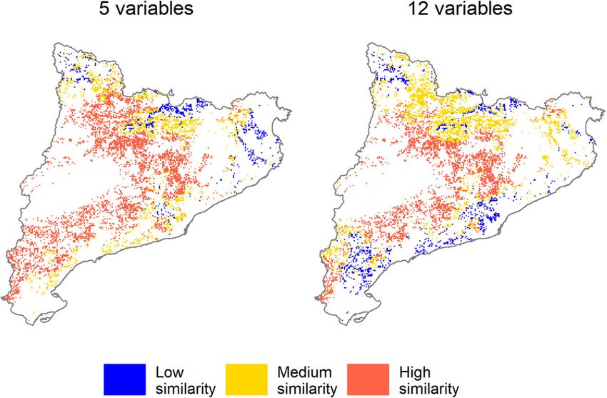
Morera et al. Forest Ecosystems   (2021) 8:21                                                                      Page 2 of 14

 (Continued from previous page)
 Conclusions: Decision tree-based models were the best approach for prediction both in sampling-like
 environments as well as in extrapolation beyond the spatial and climatic range of the modeling data. In this study,
 we show that proper variable selection is crucial to create robust models for extrapolation in biophysically
 differentiated areas. This allows for reducing the dimensions of the ecosystem space described by the predictors of
 the models, resulting in higher similarity between the modeling data and the environmental conditions over the
 whole study area. When dealing with spatial-temporal data in the analysis of biogeographical patterns,
 environmental blocking is postulated as a highly informative technique to be used in cross-validation to assess the
 prediction error over larger scales.
 Keywords: Modeling, Regression, Biogeography, Climate, Forest, Fungi, Mushrooms

Background                                                       2017; Bonete et al. 2020). Yet, many machine learning
Understanding the biogeographical patterns of organisms          algorithms have been developed in recent years, and each
in natural ecosystems and predicting their distribution is a     of them may be more or less appropriate depending on
fundamental challenge in environmental sciences (Ehrlén          the specific tasks and research objectives (Thessen 2016).
and Morris 2015). This entails a deep understanding of           This highlights the need for systematic studies allowing
their distribution across space and time underpinning            for discerning the most suitable methodology according to
ecological mechanisms, which becomes increasingly                a given research objective and data. Although several stud-
complex with an increasing amount of factors driving             ies have analysed the performance of different analytical
these patterns and the possible interactions and nonlinear       approaches (Hill et al. 2017; Bonete et al. 2020; Mayfield
dependencies between them (Dixon et al. 1999; Ye et al.          et al. 2020), existing ecological research addressing sys-
2015). Such complex interrelationships require advanced          tematic assessments and comparisons of alternative mod-
data analytic methods and modeling tools to yield realistic      eling and predictive methods is scarce, making it difficult
predictions of natural ecosystem attributes and processes.       to provide clear methodological recommendations about
  Statistical methods traditionally used for this purpose        the suitability of different approaches. Besides, in the field
aim at accounting for several elements that govern these         of environmental sciences, often, extrapolations in biophy-
natural mechanisms, trying to reach a parsimonious and           sically differentiated areas are required, which makes it ne-
robust understanding of ecological patterns (Wood and            cessary to take even more into account the data spatial
Thomas 1999). However, since conventional parametric             dependencies. Due to data spatial autocorrelation, random
approaches may over-simplify nonlinear relationships             cross-validations leads to over-optimistic error estimates
between variables and over- or under-estimate the influ-         (Bahn and McGill, 2012; Micheletti et al., 2013; Juel et al.
ence of some drivers, conventional parametric approaches         2015; Gasch et al. 2015; Roberts et al. 2017; Meyer et al.
may result in poor predictions and/or descriptions of            2018; Meyer et al. 2019a), which makes it necessary to use
reality (Ye et al. 2015), especially for the analyses of large   proper, complementary validation methods such as spatial
databases. To overcome potential limitations of classic          cross-validation (Le Rest et al. 2014; Pohjankukka et al.
statistical approaches in big data analysis, the increased       2017; Roberts et al. 2017; Meyer et al. 2018; Valavi et al.
computing power has led to recent considerable growth in         2018). Moreover, spatial dependencies in the data can lead
the use of analytical methods based on artificial intelligence   to a misinterpretation of some predictors outside the sam-
such as machine learning (Christin et al. 2019).                 pling range (Meyer et al. 2018, 2019a).
  Machine learning algorithms are increasingly being               Biogeographical patterns of fungal dynamics over large
used in species distribution and ecological niche modeling       scales are a highly relevant question in ecology given the
(Prasad et al. 2006; Cutler et al. 2007; Hannemann et al.        key role of fungi in forest ecosystems (Stokland et al. 2012;
2015; Liang et al. 2016; Prasad 2018; Gobeyn et al. 2019),       Mohan et al. 2014), especially in fungi-tree symbiosis.
forest resources (Stojanova et al. 2010; Görgens et al.          However, due to their great diversity and differential eco-
2015) and climate change studies (Thuille 2003; Bastin           logical requirements (Glassman et al. 2017), as well as the
et al. 2019), among others. To determine to what extent          difficulty of monitoring their dynamics and the large array
these “new” methodologies can contribute to improving            of potential drivers (Büntgen et al. 2013), little is known of
our understanding and prediction capacity within the field       fungal dynamics over large scales. The prediction of biogeo-
of environmental sciences, comparative studies are re-           graphical patterns of fungal dynamics requires large fungal
quired between those models that have been used histor-          datasets with a correct taxonomic identification of the
ically and those fed by artificial intelligence algorithms       specimens and a consistent sampling methodology across
(Özçelik et al. 2013; Diamantopoulou et al. 2015; Hill et al.    space and time to avoid sample bias (Hao et al. 2020).
Morera et al. Forest Ecosystems   (2021) 8:21                                                                      Page 3 of 14

  In particular, the spatially-explicit prediction of fungal   types considered in this study were the main Mediterranean
productivity, i.e. mushroom fruiting patterns, is a key        pine forest ecosystems that represent the majority of the
feature of fungal dynamics as it is tightly related to the     forest area of the study region, namely, pure stands of Pinus
supply of multiple provisioning, regulating and cultural       halepensis, P. sylvestris, P. pinaster, P. nigra and P. uncinata
ecosystem services (Boa 2004). However, the high correl-       and mixed stands of P. halepensis and P. nigra, and of P.
ation between mushroom production and meteoro-                 sylvestris and P. nigra. We used a dataset that contains
logical conditions among other drivers (Taye et al. 2016;      information from 98 permanent monitoring plots for fungal
Alday et al. 2017; Collado et al. 2019) makes the predic-      dynamics sampled on a weekly basis during the main
tion of mushroom production challenging, especially in         mushroom fruiting period, between August and the end of
Mediterranean ecosystems where there is a high inter-          December and from 1997 to 2019. The plots were distrib-
annual variability of climatic conditions. The long period     uted randomly and proportionally to the relative surface of
of potential fruiting of different mushroom species, as a      the different pine forest ecosystems (Bonet et al.
result of their adaptation to the recurrent climatic           2010) (Fig. S1). Data were aggregated to an annual
patterns of a dry summer followed by a wet autumn              basis to create predictive models to estimate annual
(Barnard et al., 2014), makes mushroom yields                  mushroom productivity. More information about the
dependent on a large number of variables. Precipitation        sampling methods and data can be found in Bonet
and temperatures on a weekly scale can be the factors          et al. (2004), Martínez de Aragón et al. (2007) and
that lengthen, shorten or shift the fruiting period (Gange     Table S3.
et al. 2007; Kauserud et al. 2008; Kauserud et al., 2009;
Büntgen et al. 2012), and also those that modulate             Climate and biophysical data
mushroom production to a higher degree (Karavani               Meteorological data for each sampling plot was obtained
et al. 2018). The large number of variables involved and       from the interpolation and altitudinal correction of daily
their presumed interactions may often yield a miscon-          weather of 201 meteorological stations from the Catalan
ception that fungal productivity is highly stochastic or       Meteorological Service and the Spanish Meteorological
very difficult to predict. Previous research to estimate       Agency. Interpolation was conducted with “meteoland”
mushroom productivity over large scales has been               R package (v0.8.1; De Cáceres et al. 2018) that uses a
mainly based on mixed-effects modeling (de-Miguel              modification of the DAYMET methodology (Thornton
et al. 2014; Sánchez-González et al. 2019). Despite being      et al. 1997; Thornton and Running 1999). Likewise, to
a valid approach, it may have certain limitations that are     determine the typical climatic conditions across the
worth assessing in comparison with alternative methods         whole study region, we used the mean of the interpo-
that remain unexplored.                                        lated daily weather variables for the period between
  This study compares different statistical and machine        1991 and 2016 with 1-km resolution. We computed the
learning models in estimating mushroom productivity at         accumulated monthly rainfall from August to October
the landscape level, together with a systematic method-        and the mean, maximum and minimum monthly
ology to determine the best approach to predict mush-          temperatures for the same period, coinciding with the
room production in forest ecosystems. Using climatic           main mushroom fruiting period.
and biophysical data together with in situ fungal records        The total area covered by the different pine forest
collected weekly over more than 20 years on a hundred          ecosystems was retrieved from the CORINE habitats
permanent plots, we developed spatially explicit, high-        map (Commission of the European Community 1991).
resolution continuous maps of mushroom productivity            The biophysical variables such as elevation, slope, aspect
that were also used in the selection of the most suitable      and stand basal area were obtained at 20-m resolution
methods for predicting this ephemeral and important            from the first cover of the LIDARCAT Project (http://
forest resource. Specifically, we compared two statistical     territori.gencat.cat/es/detalls/Article/Mapes_variables_
models, namely, generalized linear mixed models (GLMM)         biofisiques_arbrat) based on different LiDAR flights
and geographically weighted regression models (GWR), as        between 2008 and 2011 with a point density of 0.5
well as four alternative state-of-the-art machine learning     points∙m− 2.
algorithms such as random forest (RF), extreme gradient
boosting (XGB), support vector machine (SVM) and artifi-       Analytical methods
cial neural network (ANN).                                     We used and compared six different analytical methods
                                                               to predict annual mushroom productivity. Two analytical
Methods                                                        approaches were based on statistical methods, namely,
Study area and sampling plots                                  generalized linear mixed-effects models (GLMM) and
The study area was Catalonia region, northeastern Spain,       geographically weighted regression (GWR), whereas the
in the western Mediterranean basin. The forest ecosystem       other four analytical methods were based on alternative
Morera et al. Forest Ecosystems (2021) 8:21 Page 4 of 14
machine learning approaches, namely, random forest (RF), yield ¼ π ðxk Þ e ln ðyieldÞ
CF ð5Þ
extreme gradient boosting (XGB), support vector machine
(SVM) and artificial neural network (ANN). where π (xk) is the probability of mushroom occurrence,
ln (yield) represents the production of mushrooms at
Statistical models fitting logarithmic scale and CF is bias correction factor.
We used a two-stage modeling approach to take into
account the high frequency of “zero” production values Generalized linear mixed models Due to mushrooms
in many sample plots over time (Hamilton and Brickell sampling methodology, where annually data was taken
1983; de-Miguel et al. 2014; Karavani et al. 2018; Collado from a network of permanent plots, we used GLMM
et al. 2018). The high occurrence of these values arise (de-Miguel et al. 2014; Karavani et al. 2018; Collado
from the small size of the plots and the stochastic nature et al. 2018). This method can consider the spatial and
of mushroom emergence (de-Miguel et al. 2014). temporal autocorrelation among observations (Pinheiro
The first stage determines the probability of mushroom and Bates 2000) adding random effects to segment the
emergence, according to binomial data of presence/ab- data into different groups according to year and plot. In
sence, using a logistic regression π(X) = E(Y|X) and a logit the proposed mixed-effects models only random effects
link function to represent the conditioned mean of Y on model interception were considered. All the models
given X (Eqs. 1 and 2). were fitted using the “glmer” function from the “lme4” R
package (v1.1–21; Bates et al. 2015).
1
π ðxk Þ ¼ E ðY jxk Þ ¼ ð1Þ
1 þ e − g ð xk Þ Geographically weighted regression GWR is a non-
stationary modeling technique that describes the
π ð xk Þ
g ðxk Þ ¼ ln ¼ β0 þ βk x k ð2Þ spatially varying relationships between the dependent
1 − π ð xk Þ variable and the explanatory variables (Wheeler and Páez
2009). Coefficients of a GWR-based model are given by
where π (xk) is the probability of mushroom occurrence,
the spatial location of data and can be estimated for any
g (xk) the logit transformation of π (xk), Y is the
new location. This means that given a grid, the esti-
dependent variable (mushroom presence/absence), xk is
mated coefficients for each point in space vary continu-
kth independent variable, β0 is the intercept parameter
ously as a function of the spatial heterogeneity of the
and βk is the regression coefficient for kth independent
relationships.
variable.
Coefficients for each regression point were calibrated
The second stage was based on the modeling of the
using the data around itself. Due to the annual sampling
production of non-zero production values at logarithmic
methodology and the geographical distribution of plots,
scale using linear regression y = E (log(Y)|X) + ε. Logarith-
some plots were grouped denser in some areas and less
mic transformation allows to limit the production range
dense in others. Consequently, we used an adaptive
in the interval [0, ∞), depending on the values of X (Eq. 3).
window according to the spatial density of our plots
The proportional bias of the logarithmic regression was
(Georganos et al. 2017). Occurrence and conditional
corrected with the Snowdon’s bias correction factor
production models, as well as the optimal data value for
(Snowdon 1991) based on the ratio of the arithmetic
adjusting the adaptive window, were obtained from the
sample mean and the mean of the back-transformed
“ggwr” and “gwr.set” functions, respectively, of the R
predicted values from the regression (Eq. 4):
package “spgwr” (v0.6–32; Bivand and Yu, 2017).
ln ðprodÞ ¼ β0 þ βk xk þ ε ð3Þ
Hyperparameters optimization of machine learning models
CF ¼ Y =^y ð4Þ To optimize the performance of machine learning
models, it was necessary to tune their respective hyper-
where ln (prod) represents the non-zero production of parameters (Hutter et al. 2011; Bergstra and Bengio
mushrooms at logarithmic scale, β0 is the intercept 2012; Duarte and Wainer 2017). This needs to be con-
parameter, βk the regression coefficient for kth independ- ducted prior to the training of the final predictive
ent variable, ε the random error of the deviation of the models and also needs to consider the spatial and tem-
observations from the conditioned mean of ln(Y) and Y/ poral dependencies of both the modeling and prediction
ŷ is the ratio between the mean of observed and the datasets (Schratz et al. 2019). Since hyperparameters
mean of predicted values of the sapling units. tuning based on a resampling method such as k-fold
Finally, the total production of mushrooms was obtained cross-validation may lead to an incorrect tuning for
from the product of the probability of appearance and the models that aim to predict in environmentally different
conditioned production of non-zero values (Eq. 5). areas (Roberts et al. 2017), hyperparameters tuning wasMorera et al. Forest Ecosystems (2021) 8:21 Page 5 of 14
conducted based on several alternative resampling specificity of the binomial classification models we used
techniques, namely, k-fold cross-validation, spatial cross- Receiver Operator Characteristic (ROC) curves, using
validation, and environmental cross-validation (Roberts the R package “ROCR” (v1.0–7; Sing et al. 2005).
et al. 2017). To assess whether GWR improved GLMM due to the
We used an optimization algorithm based on a search non-stationary nature of data and to avoid introducing
grid (Bergstra and Bengio 2012) implemented in the R an improvement that was not attributed to the type of
package “mlr3tuning” (v0.5.0; Becker et al. 2020) that se- modeling, the same explanatory variables as in GLMM
lects the best hyperparameters configuration according were used. To test the non-stationarity of the independ-
to a given metric. The search space was defined from ent variables of GWR models, the local parameters were
the Cartesian product of the discretized values of a set compared with global GLMM coefficients. The probabil-
of n hyperparameters to be tuned in each model ity of incorporating non-stationary variables increases if
(Table 1). First, a set of hyperparameters configurations the estimated coefficient of the variable in GLMM (±
from the search grid was randomly selected and evalu- standard error) is outside the 1st and 3rd quartile of the
ated according to each resampling strategy. A search GWR model coefficient (Propastin 2009).
grid of resolution 25 was defined and tested with a total For each of the four machine learning algorithms, two
of 250 different hyperparameters configurations. Other- models were adjusted. The first ones were trained using
wise, we used 10 folds in each resampling strategy using a total of 15 biophysical variables, while the second ones
the R package “mlr3” (v0.9.0; Lang et al. 2019) for the were trained using a subset of them (Table S1). This
core computational operations and the extensions subset was determined from the same five variables used
“mlr3spatiotempcv” (v0.1.1; Schratz and Becker 2021) in the statistical models, including climate predictors
and “mlr3learners” (v0.4.3; Lang et al. 2020a) for the re- only. This allowed us to assess separately the prediction
sampling and the use of the different models, respect- accuracy due to the analytical method, and the predic-
ively. In addition, the R packages “paradox” (v0.6.0; Lang tion accuracy due to differences between predictors or
et al. 2020b) and “mlr3keras” (v0.1.3; Pfisterer et al. the number of explanatory variables. The final machine
2021) were also used in hyperparameters tuning. learning models were trained using 100% of the sampled
data (henceforth referred to as “modeling data”) and the
Model and variable selection and evaluation optimal hyperparameters settings. We used the opti-
Statistical model evaluation and variable selection was mized hyperparameters from an environmental blocking
based on the current knowledge of forests and (Roberts et al. 2017) to train the final models. The rela-
mushroom ecology, the statistical significance of model tionship between predictors and mushroom productivity
parameters (p < 0.05 or t > |1.96|), the variance inflation was assessed based on partial dependence plots (PDPs),
factor (VIF) to quantify the severity of multicollinearity a low-dimensional graphical rendering between variable
and the parsimony principle. To check the sensitivity/ pairs, in order to determine whether this relationship
lacked ecological sense. The importance of the predictors
Table 1 Hyperparameters ranges and types for each machine
of the models was determined from a sensitivity analysis
learning model
using the R package “rminer” (v1.4.2; Cortez 2016).
Algorithm Hyperparameter ID Type Lower Upper
RF mtry Integer 1 N° of predictors Evaluation of the predictive performance and mapping
min.node.size Integer 1 100 Since the main purpose of this study was to develop
num.trees Integer 2 500 models to accurately predict mushroom productivity,
XGB nrounds Integer 1 100 this entails the evaluation of the predictive performance
gamma Numeric 1 25
of the resulting models also outside of the range of the
training (or fitting) region. With the aim of determining
max_depth Integer 1 15
the similarities between modeling data and the environ-
eta Numeric 0.1 1 mental conditions of the whole study area, a principal
SVM cost Numeric 1 50 component analysis (PCA) based on both datasets
gamma Numeric 0.1 1 altogether was used. Using the location of the modeling
ANN epochs Integer 1 100 data within the space described by the first two compo-
batch_size Integer 1 N° observations
nents of the PCA, a density map was created based on a
two-dimensional kernel density estimation and imple-
“Hyperparameter id” corresponds to the names specified in the R package
used to train each model. RF (random forest), XGB (extreme gradient mented in the “kde2d” function of the R package “MASS”
boosting), SVM (support vector machine), and ANN (artificial neural network) (Venables et al. 2002). By overlapping this density map
models were trained using the R packages “ranger” (v0.12.1; Wright and
Ziegler 2017), “xgboost” (v0.90.0.2; Chen et al. 2019), “e1071” (v1.7–2; Meyer
and the location of each pixel of the study area within the
et al. 2019b) and “keras” (v2.3.0.0.0; Allaire and Chollet 2019), respectively space defined by the two principal components of theMorera et al. Forest Ecosystems (2021) 8:21 Page 6 of 14
PCA, a similarity value (ranging from 0 to 1) was obtained models also showed a statistically significant and nega-
for each pixel of the study area based on the modeling tive relationship with the maximum temperature of
data density. This similarity value was classified in three August and October, respectively (Tables S1, S2, S3).
categories: low [0, 0.1], medium (0.1, 0.3] and high (0.3, 1] Yet, the coefficients of GWR models varied according to
similarity. This classification mainly aimed at detecting geographical location (Table S3 and Fig. S2), describing
the areas with very low similarity, i.e. with very different certain non-stationarity in both precipitation and
climatic conditions compared to the modeling data. This temperature.
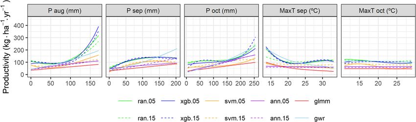
whole procedure was performed separately using the 5 Within GLMM models, PDPs showed an almost linear
climatic predictors of the 5-variable models and the 12 relationship between the amount of precipitation be-
climatic predictors of the 15-variable models, respectively. tween August and October and mushroom productivity
To evaluate and compare the predictive accuracy of in the model fit data range. In contrast, GWR showed
the models, different resampling strategies were used an accelerated growth in productivity by increasing
(see the section of Hyperparameters optimization of rainfall, which was accentuated in those locations with a
machine learning models). The MSE and bias2 of the higher precipitation regression coefficient. Besides, and
models were estimated by averaging, respectively, over similarly in GLMM and GWR, the maximum temperature
the MSE and bias2 obtained from each of the 10 folds in August showed a decelerated decrease in productivity by
for each cross-validation strategy. increasing temperature, while the maximum temperature
To generate the landscape-level mushroom productiv- of October, even though it showed a negative relation,
ity maps we used the predictions of the final trained resulted in little relevance in mushroom productivity for
models. These maps were constructed with a resolution the range of values of the fitting data (Fig. 1).
of 1 km in accordance with the resolution of the climatic Different machine learning models resulted in rather
data. The resulting maps were evaluated on the basis of similar relationships between variables although, due to
the scientific and expert knowledge about biogeographical the particularities of each algorithm, the patterns
fungal productivity patterns in order to assess whether changed slightly between approaches. In contrast to the
they followed ecologically logical patterns (related to relationships in GLMM and GWR models, some of the
climatic conditions). Thus, we would expect smoothed machine learning models did not show monotonically
estimates across the territory driven by the variations of increasing or decreasing relationships between dependent
the most important predictors of each model. and explanatory variables. This monotony was often
broken at the extremes of the range of values of the
Results predictor variables, where the amount of data to train the
Relationships between dependent and explanatory models was lower (Fig. 1). Moreover, machine learning
variables methods also showed differences in the importance
Statistical models showed a statistically significant and assigned to different predictors. Thus, XGB identified
positive relationship of mushroom productivity with some variables as very important compared to other
rainfall in August, September and October (both in predictors. Specifically, in the models trained with 15
conditioned production and occurrence models). On the variables, XGB showed a greater importance of precipita-
other hand, conditioned production and occurrence tion in August, September and October, minimum
Fig. 1 Relationship between annual mushroom productivity and August, September and October precipitation and maximum temperatures in
September and October (these variables are the variables used in the statistical models and the five variables machine learning models). ran
(random forest), xgb (extreme gradient boosting), svm (support vector machine), ann (artificial neural network), glmm (generalized linear mixed
models) and gwr (geographically weighted regression). 05 and 15 refer to the models trained with five and fifteen variables, respectivelyMorera et al. Forest Ecosystems (2021) 8:21 Page 7 of 14
temperature in October and aspect. In addition, precipita- Within ML models, ANN models showed a higher error
tion of August resulted in having further greater import- than the other algorithms. Decision tree-based models,
ance in the models trained with five variables. Conversely, namely, RF and XGB, showed no differences between
the importance detected by RF and SVM to the whole the 15- and five-variable models when k-fold CV-based
array of predictors was more homogeneous. RF showed a resampling was used. Using an environmental blocking,
greater importance to the same variables as XGB, while RF models, as well as SVM and ANN, showed lower ac-
the most important variables in SVM were precipitation curacy when using five variables instead of 15. Contrary,
in September and October, average temperature in August the prediction error using XGB increased significantly
and September, and minimum temperature in August when using 15 variables (instead of five) in the environ-
(Fig. 2). mental CV, resulting in the lowest accuracy among all
GLMM and GWR fitted models and their coefficients are machine learning models and equaling the error of the
shown in the supplementary material in Table S1 to S3. statistical models. Decision tree-based models reduced
Likewise, optimal machine learning hyperparameters can be significantly the bias between predicted and observed
found in the supplementary material in Tables S4 and S5. values, especially when conducting k-fold CV. On the
other hand, the error estimated from a spatial CV with
Predictive accuracy of different methods the SVM and ANN models trained with 15 variables was
In general, ML models showed better predictive accur- lower than in the five-variable models. Using a k-fold
acy, in terms of MSE, compared to the statistical models. CV, the error of the SVM models was higher when using
Fig. 2 Standardized variable importance value used to train random forest (ran), extreme gradient boosting (xgb) and support vector machine
(svm) models with five a and 15 b variables. Variable importance values represent the contribution of each variable in the prediction of annual
mushroom productivityMorera et al. Forest Ecosystems (2021) 8:21 Page 8 of 14
more predictors, whereas in the ANN models it was beyond the range of the modeling data. Specifically,
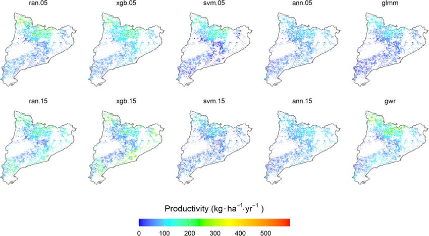
higher when using more parsimonious models. Although the similarity map based on 12 predictors, shows that
GWR improved GLMM predictive accuracy in the k-fold the number of pixels with low and medium similarity
and spatial CV mainly due to a notable bias reduction, this increased by 58% (359 km2) and 50% (847 km2), re-
was not the case in the environmental CV, where the error spectively, compared to the similarity map based on
was similar for both statistical modeling approaches five predictors. On the other hand, pixels with high
(Table 2). similarity decreased by 28% (1206 km2).
Decision tree-based models increased the predictive RF, XGB and SVM trained with 15 variables also
accuracy reducing MSE by up to 10% compared to XGB, resulted in less smoothed predictions of mushroom yield
almost by 40% compared to ANN and GLMM, and by across the territory compared to estimates based on the
20% compared to GWR when using k-fold CV. Similar subset of five predictors. Furthermore, SVM produced
trends were also obtained using environmental and illogical predictions below 0 kg·ha− 1·year− 1 in a few
spatial CV. spatially localized areas when five variables were used, and
scattered throughout the territory when using 15 predic-
Mapping and accuracy of predictions at the landscape tors. In contrast, ANN resulted in very smoothed esti-
level mates across the territory, contrary to the maps obtained
The spatially explicit predictions from each model at the from all the other machine learning methods (Fig. 3).
landscape level resulted in rather similar general patterns In addition, mushroom productivity predictions based
between modeling approaches (Fig. 3). Namely, they on RF, XGB, SVM and GWR ranged between 0, in the
predicted higher productivity in the northern areas of less productive areas, and approximately 300 and 400
the study region, characterized by higher altitudes, i.e., kg·ha− 1·year− 1 (with some maximum peaks reaching 500
Pyrenees mountain range. Also, the different models and 600 kg·ha− 1·year− 1). Slightly lower productivity was
reproduced similar patterns within these areas according detected using GLMM and ANN for the most productive
to variations in local topography. In addition, RF, XGB sites, i.e. not exceeding 200 kg·ha− 1·year− 1 in any point of
and SVM models trained with 15 predictors yielded the study area.
higher estimates of mushroom productivity in coastal
areas compared to the same algorithms based on a sub- Discussion
set of five predictors. Those coastal areas represented To our knowledge, this is the first study addressing a
the least similar bioclimatic conditions compared to the systematic evaluation of the predictive performance of
modeling data when using 12 predictors (Fig. 4 and alternative statistical and machine learning models to
Fig. S3), therefore increasing the area of extrapolation predict fungal productivity, and one of the few system-
atic comparisons between these different predictive
Table 2 Mean squared error (MSE) and squared bias (bias2) of approaches within the field of ecological research. This
the different machine learning and statistical models depending was conducted using one of the largest datasets (if not
on different resampling strategies, namely, k-fold, environmental, the largest one) for fungal productivity monitoring,
and spatial cross-validation. ran (random forest), xgb (extreme based on consistent sampling methodology and taxonomic
gradient boosting), svm (support vector machine), ann (artificial identification of mushrooms over more than 20 years on
neural network), glmm (generalized linear mixed models) and gwr nearly a hundred permanent sampling plots, randomly dis-
(geographically weighted regression). 05 and 15 refer to the tributed throughout the study region, which contributes to
models trained with five and fifteen variables, respectively overcoming most of the practical problems related to the
Environmental cv Spatial cv k-fold cv existence of available data for modeling fungal resources
MSE Bias2 MSE Bias2 MSE Bias2 (Hao et al. 2020).
ran.05 22,941 88 18,096 37 12,677 1 When dealing with complex ecological interactions
ran.15 19,875 33 18,356 10 12,148 2 between multiple potential explanatory variables, our
xgb.05 21,778 178 17,433 62 13,744 1
results show that statistical models, especially GLMM,
clearly seem to have lower predictive performance
xgb.15 28,654 148 18,473 93 13,231 1
compared to artificial intelligence-based approaches,
svm.05 30,901 2556 19,930 1226 14,140 657 in line with previous research (e.g. Smoliński and
svm.15 22,910 1214 21,032 797 12,824 392 Radtke 2016 and Schratz et al. 2019). They were less
ann.05 28,950 5206 25,021 4511 20,128 3087 accurate and produced large over- or underestimation
ann.15 26,815 5619 29,516 8033 24,487 5946 of mushroom productivity (Table 2), making them
glmm 28,318 9528 24,460 5228 21,086 3394
unreliable for such purposes compared to other alter-
natives. On the other hand, statistical models can be
gwr 28,214 9789 20,590 2553 16,078 204
good candidates for detecting the most appropriateMorera et al. Forest Ecosystems (2021) 8:21 Page 9 of 14 Fig. 3 Landscape-level prediction of total annual mushroom productivity, using ran (random forest), xgb (extreme gradient boosting), svm (support vector machine), ann (artificial neural network), glmm (generalized linear mixed models) and gwr (geographically weighted regression). 05 and 15 labels refer to the models trained with five and fifteen variables, respectively variables to be used in machine learning models and of probability distributions to be correctly approxi- unravel environmental-ecological relationships be- mated. Fitting GWR parameters using a subset of tween them (Shmueli 2010; Schratz et al. 2019), since data according to their geographical location cor- the inherent statistical assumptions that shape these rected for the strong underestimation of fungal models allow the relationships between data in a set productivity produced by GLMM models using k-fold Fig. 4 Similarity between the climate conditions of the whole study area and the modeling data. The spatial similarity was based on the number of sampled data with an environment similar to the prediction environment. The per-pixel similarity was obtained by overlapping the pixel position and a density map of the sampled data in a two-dimensional space defined by the first two principal components of a principal component analysis (PCA). The PCA was performed with five and 12 variables according to the machine learning models’ climate predictors (Fig. S3)
Morera et al. Forest Ecosystems   (2021) 8:21                                                                 Page 10 of 14

CV. However, it was not possible to correct for the           result in greater extrapolation beyond the range of the
bias in mushroom productivity prediction in environ-          modeling data, as shown in our study (Fig. 4 and Fig. S3).
mentally differentiated areas. By considering spatial         Thus, in the 15-variable models, extrapolation beyond the
parameters, we were able to find non-stationary pat-          range of modeling data occurred over a larger extent of
terns across the territory, denoting that climatic con-       the study area compared to the models based on five
ditions do not affect equally at a landscape level.           predictors. Assuming that k-fold CV estimates model
   As demonstrated here, choosing a subset of variables       accuracy in areas where climatic conditions are similar to
from statistically significant predictors from statistical    the modeling data, while environmental or spatial CV esti-
models can help us to deal with some drawbacks. A             mates model prediction error in climatically different
problem with selecting a single subset of variables from      areas (Roberts et al. 2017; Meyer et al. 2019a), the assess-
a machine learning models is that, due to the algorithm       ment of model accuracy for prediction across the study
itself, the significance is adjusted differently and could    area can be improved based on the similarity in the
be inappropriate for some of them. For example, within        climatic conditions between the modeling data and the
decision tree algorithms, XGB determines the variable to      whole study area. Thus, random blocking with five-
be used in each node of the tree among the total of           predictor models informed more appropriately about the
variables of a model, while RF does it within a subset of     magnitude of the prediction error over a larger area com-
them, giving greater probability of being chosen to those     pared to 15-predictor models, because areas with high
less important variables (Hastie et al. 2001). On the         similarity increased when using fewer predictors, i.e. from
other hand, the importance of a set of correlated vari-       ~ 2800 to ~ 4000 km2. Conversely, the prediction error of
ables can be distributed among the different predictors       the less parsimonious models will be given by an environ-
(giving lower importance to each one of them), but the        mental blocking in a smaller area than in the models with
total importance that this set represents in the predictive   less predictors. To assess which model is more suitable for
performance is remarkable (Toloşi and Lengauer 2011).         prediction, one needs to consider the extent of the study
This can cause that when discarding the less important        area where the prediction error is quantified through
variables, this set of predictors is omitted, causing a       random blocking and through environmental block-
notorious drop in predictive performance. Moreover, in        ing, respectively, and not only whether the model
a group of correlated variables where there is only one       error of more or less parsimonious models is higher
true predictor (the one that implies real causality),         or lower in each blocking strategy. In our study,
machine learning algorithms could give similar values of      when using models with 15 predictors, the entire
importance to the whole set of variables (Archer and          coastal areas (east) and the Pyrenees mountain range
Kimes, 2008), actually hiding the true predictor. These       (north), showed a low to moderate similarity of
problems may be aggravated when using a larger num-           climatic conditions compared to the modeling data.
ber of variables to train the models, where the probabil-     In contrast, in the 5-predictor models, the coastal
ity of finding groups of correlated variables is higher.      areas with low similarity decreased, while the area
Consequently, each machine learning algorithm give a          with high similarity of the Pyrenean mountain range
different importance to each variable. Therefore, to iden-    increased considerably. Thus, it seems that parsimony
tify the variables that could best explain the processes      may be a useful model selection criterion not only
that occur in natural ecosystems and/or use the variable      for statistical methods but also for machine learning
importance to select a subset of predictors to train a        algorithms (Coelho et al. 2018).
more parsimonious model, the above considerations                As noted, statistical models do not seem to be com-
should be taken into account.                                 petitive compared to machine learning approaches due
   The fact that the prediction error obtained from RF,       to poor predictive performance. Among the machine
SVM, and ANN models was lower when using 15 pre-              learning models, the ANN approach had the highest
dictors in environmental blocking, suggests that models       prediction error and also resulted in biogeographic
using a larger number of predictors may be a better           patterns that did not seem to agree with the expected
alternative for predicting mushroom productivity at the       climatic variations throughout the study area. In turn,
landscape level. However, the combination of climatic         SVM yielded illogical negative values of mushroom
conditions represented by model predictors increases          productivity in some areas. Therefore, the best candi-
exponentially with increasing number of variables             date methods are the decision trees-based algorithms,
(Hughes, 1968). This makes it more likely that increasing     i.e. RF and XGB. Considering the similarities in the
the number of model predictors will increase the              climatic conditions between the modeling data and the
mismatch between the modeling data and the climatic           whole study area, we conclude that the best models will
conditions across the whole study area. Therefore,            be RF and XGB models trained with five predictors.
models with a larger number of predictors will probably       This study shows that, although machine learning
Morera et al. Forest Ecosystems   (2021) 8:21                                                                                  Page 11 of 14

algorithms allow to train models using a large number          areas to further assist model selection and proper
of variables, it may be wise to conduct a more thorough        characterization of the prediction error based on alterna-
selection of model predictors prior to training the final      tive resampling techniques. In the end, given the multiple
models (Kuhn and Johnson 2013). This further contrib-          environmental factors driving fungal productivity, we
utes to improving the selection of the best modeling           highlight the importance of applying such methods using
approach for prediction and also provides a method-            high-resolution environmental information to properly
ology that, in the face of the current paucity of data to      estimate its biogeographic patterns over large scales.
build process-based models (Hao et al. 2020), can be
reasonably used in extrapolation. This is especially           Abbreviations
                                                               ANN: Artificial Neural Network; bias2: Squared bias; GLMM: Generalized Linear
relevant in a context of global change, where climatic         Mixed Models; GWR: Geographically Weighted Regression; MAE: Mean
conditions are predicted to change over the years              Absolute Error; PCA: Principal Component Analysis; PDP: Partial Dependence
beyond the historical climatic ranges.                         Plots; RF: Random Forest; MSE: Mean Squared Error; SVM: Support Vector
                                                               Machine; XGB: Extreme Gradient Boosting

Conclusions
This study compares different statistical and machine          Supplementary Information
learning models for predicting fungal productivity             The online version contains supplementary material available at https://doi.
                                                               org/10.1186/s40663-021-00297-w.
biogeographical patterns using a systematic methodology.
Decision tree-based models, namely, RF and XGB,                 Additional file 1: Table S1. Fixed GLMM coefficients. β1, β2, β3
performed the best in the prediction of fungal productivity     significance were calculated from t-value, while β3, β4, β5 from p-value.
in both environmentally similar and differentiated areas.       Table S2. Random GLMM coefficients. Table S3. GWR models
                                                                coefficients. Table S3. Summary of mushroom, climate and physical data
Therefore, we recommend the use of these algorithms for         of the 98 sampled plots. All these variables were used to train the 15-
further research involving the prediction of fungal prod-       variable machine learning models, while the 5-variable machine learning
uctivity, both under the current bioclimatic conditions         models and the statistical models only used those marked with *. The re-
                                                                sponse variable is shown with **. Table S4. Tuned optimal hyperpara-
and under climate change scenarios. When using these            meters using a k-fold CV. Table S5. Tuned optimal hyperparameters
methods, careful selection of predictors allows for defining    using an environmental CV. Figure S1. Study area, distribution of mush-
more interpretable and computationally less expensive           room productivity monitoring plots (red points) and pine forest ecosys-
                                                                tems represented by the sample plots (green area) Coordinates system:
models as well as for reducing the environmental space          WGS 84 / UTM zone 31 N. Figure S2. GWR coefficient estimates accord-
described by model predictors. Accordingly, the range of        ing to geographical location. Coefficient of precipitation amount from
environmental conditions represented by the predictors in       August to October (A) and maximum temperature in August (B) in condi-
                                                                tioned production model. Coefficient of precipitation amount from Au-
the modeling data can be more similar to the conditions         gust to October (A) and maximum temperature in October (D) in
over the whole study area, leading to reduced extrapola-        occurrence model (C). Figure S3. Similarity in climatic conditions be-
tion. As a result, predictions can be more ecologically con-    tween the modeling data and the whole study area using five or 12 vari-
                                                                ables. Two-dimensional representation given by the two principal
sistent compared to models with much higher number of           components, namely, PC1 and PC2, of a principal component analysis
predictors. In this regard, the degree of similarity in the     (PCA) of the modeling data (with a density map) and the environmental
range of environmental conditions between the modeling          conditions over the whole study area (gray dots).
data and the whole study area for prediction is relevant
when selecting the most appropriate blocking strategy for      Acknowledgements
estimating model error. In more parsimonious models,           Not applicable.
where the range of the modeling data may be more repre-
sentative of the environmental conditions over the whole       Authors’ contributions
                                                               JMdA, JAB and SdM contributed in the installation of the sampling plots and
study area compared to more complex models, the magni-         data collection. AM, SdM and JL analysed the data. AM wrote the
tude of the prediction error at the landscape level may be     manuscript. All authors participated in the review and editing of the
better retrieved through random blocking. In contrast, in-     manuscript. SdM supervised the work during the whole process. The authors
                                                               read and approved the final manuscript.
creasing model complexity may require environmental
blocking for a more proper characterization of the predic-     Funding
tion error at the landscape level. Model and variable          This work was supported by the Secretariat for Universities and of the
selection should therefore also consider the extent of the     Ministry of Business and Knowledge of the Government of Catalonia and the
                                                               European Social Fund. This work was partially supported by the Spanish
area within the study region where the magnitude of the        Ministry of Science, Innovation and Universities (Grant No. RTI2018–099315-
prediction error can be quantified more appropriately          A-I00). J.A.B. benefitted from a Serra-Húnter Fellowship provided by the
from either environmental or random blocking. Maps             Government of Catalonia.
depicting the similarity between the environmental condi-
tions accounted by the modeling data compared to the en-       Availability of data and materials
                                                               The datasets generated and/or analyzed during the current study are not
vironmental conditions of the whole study area, can be         publicly available due to legal constraints because they are owned by different
useful to identify environmentally different or similar        institutions, but are available from the authors on reasonable request.
Morera et al. Forest Ecosystems (2021) 8:21 Page 12 of 14
Declarations Büntgen U, Peter M, Kauserud H, Egli S (2013) Unraveling environmental drivers
of a recent increase in Swiss fungi fruiting. Glob Chang Biol 19(9):2785–2794.
Ethics approval and consent to participate https://doi.org/10.1111/gcb.12263
Not applicable. Chen T, He T, Benesty M, Khotilovich V, Tang Y, Cho H, Chen K, Mitchell R, Cano I,
Zhou T, Li M, Xie J, Lin M, Geng Y, Li Y (2019) Xgboost: extreme gradient
boosting. R package version 0.90.0.2. https://CRAN.R-project.org/package=
Consent for publication xgboost. Accessed 10 Nov 2020
Not applicable. Christin S, Hervet É, Lecomte N (2019) Applications for deep learning in ecology.
Methods Ecol Evol 10:1632–1644. https://doi.org/10.1111/2041-210X.13256
Coelho MTP, Diniz-Filho JA, Rangel TF (2018) A parsimonious view of the
Competing interests parsimony principle in ecology and evolution. Ecography. https://doi.org/1
The authors declare that they have no competing interests. 0.1111/ecog.04228
Collado E, Bonet JA, Camarero JJ, Egli S, Peter M, Salo K, Martínez-Peña F,
Author details Ohenoja E, Martín-Pinto P, Primicia I, Büntgen U, Kurttila M, Oria-de-Rueda JA,
1
Department of Crop and Forest Sciences, University of Lleida, Av. Alcalde Martínez-de-Aragón J, Miina J, de-Miguel S (2019) Mushroom productivity
Rovira Roure 191, E-25198 Lleida, Spain. 2Joint Research Unit trends in relation to tree growth and climate across different European forest
CTFC-AGROTECNIO-CERCA Center, Av. Rovira Roure 191, 25198 Lleida, Spain. biomes. Sci Total Environ. https://doi.org/10.1016/j.scitotenv.2019.06.471
3
Forest Science and Technology Centre of Catalonia, Ctra. Sant Llorenç de Collado E, Camarero JJ, Martínez de Aragón J, Pemán J, Bonet JA, de-Miguel S
Morunys km 2, 25280 Solsona, Spain. 4Forest Advanced Computing and (2018) Linking fungal dynamics, tree growth and forest management in a
Artificial Intelligence Laboratory, Department of Forestry and Natural Mediterranean pine ecosystem. Forest Ecol Manag 422:223–232. https://doi.
Resources, Purdue University, West Lafayette, IN 47907, USA. org/10.1016/j.foreco.2018.04.025
Commission of the European Community (1991) CORINE biotopes manual –
Received: 27 November 2020 Accepted: 22 February 2021
habitats of the European Community. DG Environment, Nuclear Safety and
Civil Protection, Luxembourg
Cortez P (2016) rminer: data mining classification and regression methods. R
package version 1.4.2. https://CRAN.Rproject.org/package=rminer
References
Allaire JJ, Chollet F (2019) Keras: R Interface to ‘Keras’. R package version 2.2.5.0. Cutler DR, Edwards TC, Beard KH, Cutler A, Hess KT, Gibson J, Lawler JJ (2007)
https://CRAN.R-project.org/package=keras. Accessed 10 Nov 2020 Random forests for classification in ecology. Ecology 88:2783–2792. https://
Alday JG, Martínez de Aragón J, de-Miguel S, Bonet JA (2017) Mushroom doi.org/10.1890/07-0539.1
biomass and diversity are driven by different spatio-temporal scales De Cáceres M, Martin-StPaul N, Turco M, Cabon A, Granda V (2018)
along Mediterranean elevation gradients. Sci Rep 7(1). https://doi.org/10.1 Estimating daily meteorological data and downscaling climate models
038/srep45824 over landscapes. Environ Model Softw 108:186–196. https://doi.org/10.101
Archer KJ, Kimes RV (2008) Empirical characterization of random forest variable 6/j.envsoft.2018.08.003
importance measures. Comput Stat Data Anal 52(4):2249–2260. https://doi. de-Miguel S, Bonet JA, Pukkala T, Martínez de Aragón J (2014) Impact of forest
org/10.1016/j.csda.2007.08.015 management intensity on landscape-level mushroom productivity: a regional
Bahn V, McGill BJ (2012) Testing the predictive performance of distribution model-based scenario analysis. Forest Ecol Manag 330:218–227. https://doi.
models. Oikos 122(3):321–331. https://doi.org/10.1111/j.1600-0706.2012. org/10.1016/j.foreco.2014.07.014
00299.x Diamantopoulou MJ, Özçelik R, Crecente-Campo F, Eler Ü (2015) Estimation of
Barnard RL, Osborne CA, Firestone MK (2014) Changing precipitation pattern Weibull function parameters for modelling tree diameter distribution using
alters soil microbial community response to wet-up under a Mediterranean- least squares and artificial neural networks methods. Biosyst Eng 133:33–45.
type climate. ISME J 9(4):946–957. https://doi.org/10.1038/ismej.2014.192 https://doi.org/10.1016/j.biosystemseng.2015.02.013
Bastin J-F, Finegold Y, Garcia C, Mollicone D, Rezende M, Routh D, Constantin Dixon PA, Milicich MJ, Sugihara G (1999) Episodic fluctuations in larval supply.
MZ, Crowther TW (2019) The global tree restoration potential. Science Science 283(5407):1528–1530. https://doi.org/10.1126/science.283.5407.1528
365(6448):76–79. https://doi.org/10.1126/science.aax0848 Duarte E, Wainer J (2017) Empirical comparison of cross-validation and internal
Bates D, Mächler M, Bolker B, Walker S (2015) Fitting linear mixed-effects models metrics for tuning SVM hyperparameters. Pattern Recognit Lett. 88:6–11.
using lme4. J Stat Softw 67:1–48. https://doi.org/10.18637/jss.v067.i01 https://doi.org/10.1016/j.patrec.2017.01.007
Becker M, Lang M, Richter J, Bischl B, Schalk D (2020) mlr3tuning: Tuning for Ehrlén J, Morris WF (2015) Predicting changes in the distribution and abundance
'mlr3'. R package version 0.5.0. https://CRAN.Rproject.org/package=mlr3 of species under environmental change. Ecol Lett 18(3):303–314. https://doi.
tuning org/10.1111/ele.12410
Bergstra J, Bengio Y (2012) Random search for hyper-parameter optimization. J Gange AC, Gange EG, Sparks TH, Boddy L (2007) Rapid and recent changes in
Mach. Learn Res 13:281–305 fungal fruiting patterns. Science 316(5821):71. https://doi.org/10.1126/
Bivand R, Yu D (2017) Spgwr: geographically weighted regression. R Pack Version science.1137489
0.6–32. https://CRAN.R-project.org/package=spgwr. Accessed 10 Nov 2020 Gasch CK, Hengl T, Gräler B, Meyer H, Magney TS, Brown DJ (2015) Spatio-
Boa E (2004) Wild edible fungi: a global overview of their use and importance to temporal interpolation of soil water, temperature, and electrical conductivity
people (non-Wood Forest products no. 17). FAO. Forestry Department, Rome, in 3D + T: the cook agronomy farm data set. Spat Stat 14:70–90. https://doi.
p 148. ISBN: 92-5-105157-7 org/10.1016/j.spasta.2015.04.001
Bonet JA, Fischer CR, Colinas C (2004) The relationship between forest age and Georganos S, Abdi AM, Tenenbaum DE, Kalogirou S (2017) Examining the NDVI-
aspect on the production of sporocarps of ectomycorrhizal fungi in Pinus rainfall relationship in the semi-arid Sahel using geographically weighted
sylvestris forests of the Central Pyrenees. Forest Ecol Manag 203(1–3):157–175. regression. J Arid Environ 146:64–74. https://doi.org/10.1016/j.jaridenv.2017.
https://doi.org/10.1016/j.foreco.2004.07.063 06.004
Bonet JA, Palahí M, Colinas C, Pukkala T, Fischer CR, Miina J, Martínez de Aragón J Glassman SI, Wang IJ, Bruns TD (2017) Environmental filtering by pH and soil
(2010) Modelling the production and species richness of wild mushrooms in nutrients drives community assembly in fungi at fine spatial scales. Mol Ecol
pine forests of the Central Pyrenees in northeastern Spain. Can J For Res 26:6960–6973. https://doi.org/10.1111/mec.14414
40(2):347–356. https://doi.org/10.1139/x09-198 Gobeyn S, Mouton AM, Cord AF, Kaim A, Volk M, Goethals PLM (2019)
Bonete IP, Arce JE, Figueiredo Filho A, Retslaff FA de S, Lanssanova LR (2020) Evolutionary algorithms for species distribution modelling: a review in the
Artificial neural networks and mixed-effects modeling to describe the stem context of machine learning. Ecol Model 392:179–195. https://doi.org/10.101
profile of Pinus taeda L. Floresta 50(1):1123. doi:https://doi.org/10.5380/rf. 6/j.ecolmodel.2018.11.013
v50i1.61764 Görgens EB, Montaghi A, Rodriguez LCE (2015) A performance comparison of
Büntgen U, Kauserud H, Egli S (2012) Linking climate variability to mushroom machine learning methods to estimate the fast-growing forest plantation
productivity and phenology. Front Ecol Environ 10(1):14–19. https://doi.org/1 yield based on laser scanning metrics. Comput Electron Agric 116:221–227.
0.1890/110064 https://doi.org/10.1016/j.compag.2015.07.004You can also read