Soil greenhouse gas fluxes from tropical coastal wetlands and alternative agricultural land uses
←
→
Page content transcription
If your browser does not render page correctly, please read the page content below
Biogeosciences, 18, 5085–5096, 2021
https://doi.org/10.5194/bg-18-5085-2021
© Author(s) 2021. This work is distributed under
the Creative Commons Attribution 4.0 License.

Soil greenhouse gas fluxes from tropical coastal wetlands and
alternative agricultural land uses
Naima Iram1 , Emad Kavehei1 , Damien T. Maher2 , Stuart E. Bunn1 , Mehran Rezaei Rashti1 ,
Bahareh Shahrabi Farahani1 , and Maria Fernanda Adame1
1 Australian  Rivers Institute, Griffith University, Nathan, QLD, 4111, Australia
2 School   of Environment, Science and Engineering, Southern Cross University, Lismore, NSW, 2480, Australia

Correspondence: Naima Iram (naima.iram@griffithuni.edu.au)

Received: 6 February 2021 – Discussion started: 19 March 2021
Revised: 24 August 2021 – Accepted: 24 August 2021 – Published: 16 September 2021

Abstract. Coastal wetlands are essential for regulating the     1   Introduction
global carbon budget through soil carbon sequestration and
greenhouse gas (GHG – CO2 , CH4 , and N2 O) fluxes. The
conversion of coastal wetlands to agricultural land alters      Coastal wetlands are found at the interface of terrestrial and
these fluxes’ magnitude and direction (uptake/release). How-    marine ecosystems and account for 10 % of the global wet-
ever, the extent and drivers of change of GHG fluxes are        land area (Lehner and Döll, 2004). They are highly produc-
still unknown for many tropical regions. We measured soil       tive and provide various ecosystem services such as water
GHG fluxes from three natural coastal wetlands – man-           quality improvement, biodiversity, and carbon sequestration
groves, salt marsh, and freshwater tidal forests – and two      (Duarte et al., 2013). For instance, mangroves can accumu-
alternative agricultural land uses – sugarcane farming and      late 5 times more soil carbon than terrestrial forests (Kauff-
pastures for cattle grazing (ponded and dry conditions). We     man et al., 2020). However, the high productivity and anoxic
assessed variations throughout different climatic conditions    soil conditions that promote carbon sequestration can also
(dry–cool, dry–hot, and wet–hot) within 2 years of mea-         favour potent greenhouse gas (GHG) emissions, including
surements (2018–2020) in tropical Australia. The wet pas-       CO2 , CH4 , and N2 O (Whalen, 2005; Conrad, 2009).
ture had by far the highest CH4 emissions with 1231 ±              The GHG emissions in coastal wetlands primarily result
386 mg m−2 d−1 , which were 200-fold higher than any other      from microbial processes in the soil–water–atmosphere in-
site. Dry pastures and sugarcane were the highest emit-         terface (Bauza et al., 2002; Whalen, 2005). The emission of
ters of N2 O with 55 ± 9 mg m−2 d−1 (wet–hot period) and        CO2 is a result of respiration, where fixed carbon by photo-
11 ± 3 mg m−2 d−1 (hot-dry period, coinciding with fertilisa-   synthesis is partially released back into the atmosphere (Oer-
tion), respectively. Dry pastures were also the highest emit-   tel et al., 2016). Emissions of CH4 result from anaerobic
ters of CO2 with 20±1 g m−2 d−1 (wet–hot period). The three     and aerobic respiration by methanogenic bacteria, mostly in
coastal wetlands measured had lower emissions, with salt        waterlogged conditions (Angle et al., 2017; Saunois et al.,
marsh uptake of −0.55±0.23 and −1.19±0.08 g m−2 d−1 of          2020). Finally, N2 O emissions are caused by denitrification
N2 O and CO2 , respectively, during the dry–hot period. Dur-    in anoxic conditions and nitrification in aerobic soils, both
ing the sampled period, sugarcane and pastures had higher       driven by nitrogen content and soil moisture (Ussiri and Lal,
total cumulative soil GHG emissions (CH4 + N2 O) of 7142        2012). Thus, the total GHG emissions from a wetland are
and 56 124 CO2-eq kg ha−1 yr−1 compared to coastal wet-         driven by environmental conditions that favour these micro-
lands with 144 to 884 CO2-eq kg ha−1 yr−1 (where CO2-eq is      bial processes, all of which result in highly variable emis-
CO2 equivalent). Restoring unproductive sugarcane land or       sions from wetlands worldwide (Kirschke et al., 2013; Oertel
pastures (especially ponded ones) to coastal wetlands could     et al., 2016).
provide significant GHG mitigation.                                Despite potentially high GHG emissions from coastal wet-
                                                                lands, these are likely to be lower than those from alterna-

Published by Copernicus Publications on behalf of the European Geosciences Union.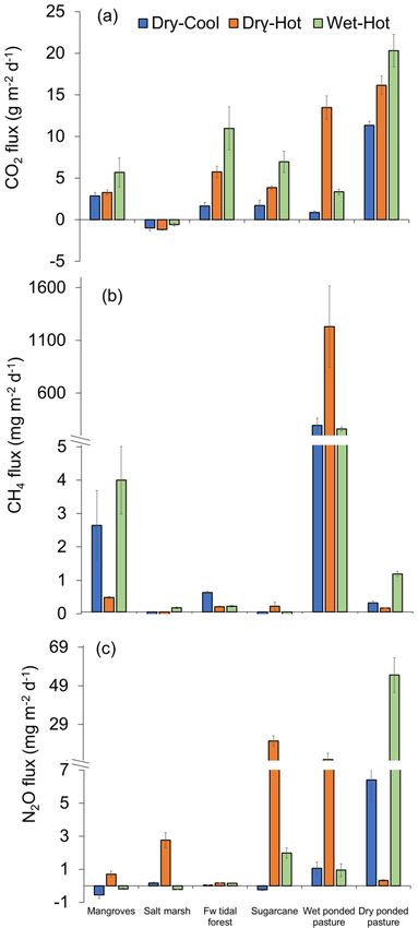
5086                                                   N. Iram et al.: Soil greenhouse gas fluxes from tropical coastal wetlands

tive agricultural land use (Knox et al., 2015), which emit               We selected five sites, including three natural coastal
GHGs from their construction and throughout their produc-             wetlands (Fig. 1) – a mangrove forest (18◦ 530 4200 S,
tive lives. Firstly, when wetlands are converted to agricul-          146◦ 150 5100 E), a salt marsh (18◦ 530 4300 S, 146◦ 150 5200 E),
tural land, the oxidation of sequestered carbon in the organic-       and a freshwater tidal forest (18◦ 530 4500 S, 146◦ 150 5200 E) –
rich soils releases significant amounts of CO2 (Drexler et al.,       and two common agricultural land use types of the region
2009; Hooijer et al., 2012). Secondly, removing tidal flow            – a sugarcane crop (18◦ 530 44.600 S, 146◦ 150 53.200 E) and a
and converting coastal wetlands to freshwater systems, such           pasture for fodder grazing. The pasture had different levels
as during the creation of ponded pastures, dams, or agricul-          of inundation: some areas were covered with shallow ponds
tural ditches, can result in very high CH4 emissions (Deemer          (50–100 cm depth); some were wet (hereafter “wet pas-
et al., 2016; Grinham et al., 2018; Ollivier et al., 2019). For       ture”; 18◦ 430 800 S, 146◦ 150 5000 E); and others were dry (here-
instance, agricultural ditches contribute up to 3 % of the to-        after, “dry pasture”; 18◦ 430 700 S, 146◦ 150 5000 E). The natural
tal anthropogenic CH4 emissions globally (Peacock et al.,             coastal wetlands and the sugarcane site were located within
2021). Finally, the use of fertilisers significantly increases        the same property < 200 m apart at Insulator Creek (Fig. 1b),
N2 O emissions (Rezaei Rashti et al., 2015). Thus, emissions          while the ponded pasture was 20 km north at Mungalla Sta-
of GHGs from land use change can be mitigated through the             tion (Fig. 1a). The mangroves were dominated by Avicennia
reversal of these activities, for instance, reduction in fertiliser   marina with a few plants of Rhizophora stylosa, and the salt
use and the reinstallation of tidal flow on unused agricultural       marsh was dominated by Suaeda salsa and Sporobolus spp.
land (Kroeger et al., 2017; Rezaei Rashti et al., 2015).              Landwards, the freshwater tidal forest, a wetland commonly
   This study measured the annual GHG fluxes (CO2 , CH4 ,             known as “tea tree swamp”, was dominated by Melaleuca
and N2 O) from three natural coastal wetlands (mangroves,             quinquenervia trees. While the mangroves and salt marsh
salt marsh and freshwater tidal forests) and two agricultural         are directly submerged by tides (5–30 cm), the freshwater
land use sites (sugarcane plantation and pasture) in tropi-           tidal forest is indirectly affected by tidal fluctuations, such as
cal Australia. The objectives were to assess the difference           during large spring tides, when tidal water can push ground-
in GHG fluxes throughout different seasons that characterise          water above the forest thus forming “supra-tidal” wetlands.
tropical climates (dry–cool, dry–hot, and wet–hot) and iden-          The coastal wetlands were adjacent to a sugarcane farm of
tify environmental factors associated with these GHG fluxes.          ∼ 110 ha (Fig. 1b). The sugarcane is fertilised once a year
These data will inform emission factors for converting wet-           with urea at a rate of 135 kg N ha−1 and harvested during
lands to agricultural land uses and vice versa, filling in a          May–June, and the foliage is left on the soil surface (trash
knowledge gap identified in Australia (Baldock et al., 2012)          blanket) after harvest. The ponded pastures in Mungalla Sta-
and tropical regions worldwide (IPCC, 2013).                          tion comprise a 250 ha farm and support ∼ 900 cattle by
                                                                      providing fodder during dry periods. The selected ponded
                                                                      pastures were covered by Eichhornia crassipes (water hy-
2     Materials and methods                                           acinth) and Hymenachne amplexicaulis (Fig. 1g–h). Each of
                                                                      the five sites was sampled during three periods: dry–cool
2.1    Study sites
                                                                      (May–September), dry–hot (October–December), and wet–
The study area is located within the Herbert River catchment          hot (January–April; Table 1). During each time period, soil
in Queensland, northeast Australia (Fig. 1a). The region has a        physicochemical properties and GHG fluxes were measured
tropical climate with a mean monthly minimum temperature              as detailed below.
from 14 to 23 ◦ C and mean monthly maximum temperature
                                                                      2.2   Soil sampling and analysis of physicochemical
from 25 to 33 ◦ C (Australian Bureau of Meteorology, ABM,
                                                                            properties
2020; 1968–2020; Sect. S4 in the Supplement). The average
rainfall is 2158 mm yr−1 , with the highest values of 476 mm          Soil physicochemical characteristics were measured in com-
during February (ABM, 2020; 1968–2020; Sect. S4). The                 posite soil samples next to each gas chamber location (n = 5;
Herbert basin covers 9842 km2 , from which 56 % is graz-              0–30 cm) for all study sites during the dry–hot season. The
ing, 31 % is conserved wetlands and forestry, 8 % is sugar-           samples were obtained by inserting an open steel corer to
cane, and 4 % is other land uses (Department of Environ-              a depth of 30 cm; the core was divided into three depths:
ment and Science, Queensland, 2013). Wetlands in this re-             0–10, 10–20, and 20–30 cm. Soil samples were oven-dried
gion were heavily deforested in the last century (1943–1996)          at 105 ◦ C for 48 h to determine volumetric water content
due to rapid agricultural development, primarily for sugar-           through gravimetric analysis. The volumetric water content
cane farming (Griggs, 2018). Before clearing, the land was            was divided by total soil porosity to determine water-filled
mostly covered by rainforest and coastal wetlands, mainly             pore space (WFPS). Total soil porosity was calculated using
Melaleuca forest, grass, and sedge swamps (Johnson et al.,            an equation from Rezaei Rashti et al. (2015; Eq. 1):
1999).
                                                                                                  soil bulk density (mg cm−3 )

                                                                      total soil porosity = 1 −                                 . (1)
                                                                                                              2.65

Biogeosciences, 18, 5085–5096, 2021                                                      https://doi.org/10.5194/bg-18-5085-2021
N. Iram et al.: Soil greenhouse gas fluxes from tropical coastal wetlands 5087
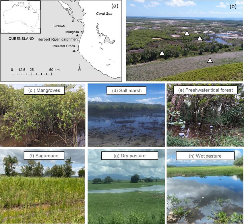
Figure 1. (a) Location of sampling sites (Insulator Creek and Mungalla) in the Herbert River catchment, northeast Australia; (b) natural
wetlands adjacent to sugarcane in Insulator Creek and sampling locations; and (c) mangroves, (d) salt marsh, (e) freshwater tidal forest,
(f) sugarcane, (g) dry pasture, and (h) wet pasture. Pictures by Naima Iram and Maria Fernanda Adame.
Table 1. Mean daily air temperature and rainfall range (Ingham, weather station 32078) during sampling.
Season Study period Daily min Daily max Rainfall
temperature (◦ C) temperature (◦ C) (mm d−1 )
Dry–cool 17 June 2018 13.4–14.6 27.7–28.2 0
Dry–hot 23–29 October 2018 15.7–21.1 32.2–36.2 0
Dry–cool 31 May to 6 June 2019 10.9–17.5 21.6–28.2 0–25
Wet–hot 17–22 February 2020 23.9–25.3 33.6–34.5 0–86
Soil texture analysis (% sand, silt, clay) was performed 2.3 Greenhouse gas fluxes
with a simplified method for particle size determination (Ket-
tler et al., 2001). Soil electrical conductivity (EC) and pH
were measured using a conductivity meter (TPS WP-84, We measured GHG fluxes (CO2 , CH4 , and N2 O) at each site
Australia) in soil–water slurry at 1 : 5. Soil subsamples were for 3 consecutive days during each sampling period except
air-dried, sieved (2 mm), ground (Retsch™ mill), and anal- for the dry–cool period of 2018, when mangroves, salt marsh,
ysed for the percentage of N (%N) and percentage of C (%C) and sugarcane were surveyed for 1 d. The sampling was car-
using an elemental analyser connected to a gas isotope ratio ried out between 09:00 and 11:00 LT, representing the mean
mass spectrometer (EA–Delta V Advantage IRMS, Griffith daily temperatures, thus minimising variability in cumula-
University). Additionally, soil samples from the top 10 cm tive seasonal fluxes based on intermittent manual flux mea-
were collected during each sampling to measure gravimetric surements (Reeves et al., 2016). Additionally, we assessed
soil moisture content and bulk density. the variability in our measurements with tidal inundation in
mangroves and salt marsh, which were regularly inundated
(∼ 10–30 cm) during the hot-dry season. However, due to lo-
https://doi.org/10.5194/bg-18-5085-2021 Biogeosciences, 18, 5085–5096, 20215088 N. Iram et al.: Soil greenhouse gas fluxes from tropical coastal wetlands
gistic constraints, further sampling was conducted only dur- GHG emission rate in a season (mg m−2 d−1 for CO2 and
ing low tides. µg m−2 d−1 for CH4 and N2 O) during low tide; and 17.38 is
We used static, manual gas chambers made of high- the number of weeks in each season, assuming these condi-
density, round polyvinyl chloride pipe, which consisted of tions were representative of the annual cycle (see Table 1).
two units: a base (r = 12 cm; h = 18 cm) and a detachable Annual cumulative soil GHG fluxes (CH4 + N2 O) were
collar (h = 12 cm; Hutchinson and Mosier, 1981; Kavehei et calculated by integrating cumulative seasonal fluxes. These
al., 2021). The chambers had lateral holes that could be left estimations did not account for soil CO2 values as our
covered with rubber bungs at low water levels and left open methodology with dark chambers only accounted for emis-
at high water levels to allow water movement between sam- sions from respiration and excluded uptake by primary pro-
pling events. When the wetlands were inundated for the ex- ductivity. The CO2-equivalent (CO2-eq ) values were estimated
periments, we used PVC extensions (h = 18 cm). Five cham- by multiplying CH4 and N2 O emissions by 25 and 298, re-
bers were set ∼ 5 cm deep in the soil; separated 1 to 2 m from spectively (Solomon, 2007), which represented the radiative
each other; and selectively located on soil with minimal veg- balance of these gases (Neubauer, 2021). For annual cumu-
etation, roots, and crab burrows. The chambers were set 1 d lative soil GHG flux calculations from coastal wetlands, we
before sampling to minimise installation disturbance during used GHG fluxes measured during low tide; therefore, our
the experiment (Rezaei Rashti et al., 2015). We were care- values did not incorporate the effect of tidal fluctuations. The
ful not to tramp around the chambers during installation and spatial and temporal replication of this study targeted spatial
sampling. The fact that emissions were not significantly dif- variation within soil type (< 50 cm, five chambers), days (3 d
ferent among days (p > 0.05) provided us with confidence per sampling), and seasons (three seasons per year). How-
that disturbance due to installation was not problematic. ever, our replication within land use and wetland type was
At the start of the experiment, gas chambers were closed. limited; thus, generalisations for all wetlands and land uses
A sample was taken at time zero and then after 1 h with a should be made acknowledging this limitation.
20 mL syringe and transferred to a 12 mL vacuumed con-
tainer (Exetainer, Labco Ltd, High Wycombe, UK). During 2.4 Statistical analyses
the dry–hot season, linearity tests of GHG fluxes with time
were conducted by sampling at 0, 20, 40, and 60 min at all GHG flux data were tested for normality through
chambers (Rezaei Rashti et al., 2016). For the rest of the ex- Kolmogorov–Smirnov and Shapiro–Wilk tests. The data
periments, linearity tests were performed in one chamber per were then analysed for spatial and temporal differences
site; R 2 values were consistently above 0.70. During each ex- with one-way analyses of variance (ANOVAs), where site
periment, soil temperature was measured next to each cham- and season were the predictive factors and the replicate
ber. For each experiment, the base depth was recorded from (chamber) was the random factor of the model. When data
five points within each chamber to calculate headspace vol- were not normal, they were transformed (log10 or 1/x) to
ume. The obtained volumetric unit concentrations were con- comply with the assumptions of normality and homogeneity
verted to mass-based units using the ideal gas law (Hutchin- of variances. Some variables were not normally distributed
son and Mosier, 1981). despite transformations and were analysed with the non-
The GHG concentrations of all samples were analysed parametric Kruskal–Wallis test and Mann–Whitney U test.
within 2 weeks of sampling with a gas chromatograph (Shi- A Pearson correlation test was run to evaluate the correlation
madzu GC-2010 Plus). For N2 O analysis, an electron capture of GHGs with measured environmental factors. Analyses
detector was used with helium as the carrier gas, while CH4 were performed with SPSS (v25, IBM, New York, USA),
was analysed on a flame ionisation detector with nitrogen as and values are presented as the mean ± standard error (SE).
the carrier gas. For CO2 determination, the gas chromato-
graph was equipped with a thermal conductivity detector. 3 Results
Peak areas of the samples were compared against standard
curves to determine concentrations (Chen et al., 2012). Sea- 3.1 Soil physicochemical properties
sonal cumulative GHG fluxes were calculated by modifying
the equation described by Shaaban et al. (2015; Eq. 2): Soil physical and chemical parameters (mean values 0–
30 cm) varied among sites (Table 2; see full results of sta-
seasonal cumulative GHG fluxes tistical analyses in Sect. S5 in the Supplement). As expected,
(mg m−2 yr−1 or µg m−2 yr−1 ) gravimetric moisture content was highest in the coastal wet-
n lands and wet pasture (> 26 %) and lowest in the sugarcane
and the dry pasture (< 14 %). All soils were acidic, espe-
X
= (Ri × 24 × Di × 17.38), (2)
i=1 cially the freshwater tidal forest and the wet pastures with
values < 5 throughout the sediment column; mangroves had
where Ri is the gas emission rate (mg m−2 h−1 for CO2 the highest pH with 6.0 ± 0.1. The lowest EC was recorded
and µg m−2 h−1 for CH4 and N2 O); Di is the mean daily in the pastures (247 ± 38 and 190 ± 39 µS cm−1 for the dry
Biogeosciences, 18, 5085–5096, 2021 https://doi.org/10.5194/bg-18-5085-2021N. Iram et al.: Soil greenhouse gas fluxes from tropical coastal wetlands 5089
and wet pasture, respectively) and highest in the three natural (0.02 ± 0.04 g m−2 yr−1 ). However, these differences were
coastal wetlands with 1418 ± 104, 8049 ± 276, and 8930 ± only significant when considering the interaction between
790 µS cm−1 for the freshwater tidal forest, salt marsh, and the time of the year and site (t = 100.21 and n = 237 with
mangroves, respectively. p < 0.001).
Soil bulk density was highest in sugarcane (1.5 ± The CH4 fluxes did not vary significantly between the
0.1 g cm−3 ) and lowest in the freshwater tidal forest (0.6 ± low and high tide within all coastal wetlands. Contrarily, for
0.1 g cm−3 ). For all sites, %C was highest in the top 10 cm salt marsh, CO2 was taken during the high tide (−1.12 ±
of the soil and decreased with depth, with the highest values 0.24 g m−2 d−1 ) but emitted (0.69 ± 0.4 g m−2 d−1 ) during
in the freshwater tidal forest (5.1 ± 0.6 %) and lowest in the the low tide (F1,28 = 20.06 with p < 0.001). Finally, for
salt marsh (1.2 ± 0.1 %). Soil %N ranged from 0.1 ± 0.0 % N2 O, fluxes differed in all coastal wetlands, with higher up-
to 0.4 ± 0.1 % in all sites, except in the freshwater tidal wet- takes in the high tide for mangroves (F1,28 = 38.28 with
land, where it reached values of 0.6 ± 0.0 % in the top 10 cm p < 0.001; F1,28 = 13.53 with p = 0.001) and higher emis-
(Table 2). sions in salt marsh (F1,28 = 38.31 with p < 0.001) during
low tide (Sect. S3). These results suggested that there was
3.2 Greenhouse gas fluxes a likely variability for CO2 and N2 O fluxes, depending on
the time of sampling.
Soil emissions for CO2 were significantly different among The wet pasture had the highest total cumulative soil GHG
sites and times of the year (t = 155.09 and n = 237 with emissions (CH4 +N2 O) with 56 124 CO2-eq kg ha−1 yr−1 fol-
p < 0.001; Fig. 2a). The highest CO2 emissions were mea- lowed by dry pasture at 23 890 CO2-eq kg ha−1 yr−1 and
sured during the wet–hot period in the dry pasture, where sugarcane at 7142 CO2-eq kg ha−1 yr−1 , while coastal wet-
values reached 20 308 ± 1951 mg m−2 d−1 , while the low- lands had comparatively lower cumulative soil GHG emis-
est values were measured in the salt marsh, the only site sions with 884, 235, and 144 CO2-eq kg ha−1 yr−1 for salt
that acted as a sink of CO2 with an uptake rate of −594 ± marsh, mangroves, and freshwater tidal forests, respec-
152 mg m−2 d−1 . In the pastures, CO2 emissions were twice tively. Overall, the three coastal wetlands measured in
as high when dry, with cumulative annual emissions of this study had lower total cumulative GHG emissions at
5748 ± 303 g m−2 yr−1 , compared to when wet, with 2163 ± 1263 CO2-eq kg ha−1 yr−1 compared to the alternate agricul-
465 g m−2 yr−1 . For the coastal wetlands, cumulative an- tural land uses, which emitted 87 156 CO2-eq kg ha−1 yr−1 .
nual CO2 emissions were highest in freshwater tidal forests
with 2213 ± 284 g m−2 yr−1 , followed by mangroves with 3.3 Greenhouse gas emissions and environmental
1493 ± 111 g m−2 yr−1 , and lowest at the salt marsh with up- factors
take rates of −264 ± 29 g m−2 yr−1 .
For CH4 fluxes, significant differences were observed Overall, we found that not one single parameter measured
among sites and seasons (t = 182.33 and n = 237 with p < in this study could explain GHG fluxes for all sites ex-
0.001). The differences between different sites were sub- cept land use. The CO2 emissions were not significantly
stantial, with wet pasture having significantly higher CH4 correlated with bulk density (R 2 = 0.026; p = 0.918; n =
emissions than any other site at rates ∼ 200 times higher 18), percent WFPS (% WFPS) (R 2 = −0.003; p = 0.99; n =
(Fig. 2b). For tidal coastal wetlands, emissions of CH4 were 18), or soil temperature (R 2 = 0.296; p = 0.233; n = 18).
highest during the wet–hot season in all the sites except Soil CH4 emissions were not correlated with bulk density
for the mangroves, which had similar emissions through- (R 2 = −0.096; p = 0.706; n = 18), % WFPS (R 2 = 0.224;
out the year (Fig. 2b). Overall, cumulative annual CH4 p = 0.372; n = 18), or soil temperature (R 2 = 0.286; p =
emissions were 209 ± 36 g m−2 yr−1 for the wet pasture 0.25; n = 18). Finally, no correlation was found between
followed by mangroves (0.73 ± 0.13 g m−2 yr−1 ), dry pas- N2 O emissions and bulk density (R 2 = −0.349; p = 0.156;
ture (0.15 ± 0.03 g m−2 yr−1 ), freshwater tidal forest (0.14 ± n = 18), % WFPS (R 2 = −0.34; p = 0.168; n = 18), or soil
0.03 g m−2 yr−1 ), salt marsh (0.04 ± 0.01 g m−2 yr−1 ), and temperature (R 2 = −0.241; p = 0.335; n = 18). The full raw
sugarcane (−0.04 ± 0.02 g m−2 yr−1 ). dataset of GHG fluxes is provided in Sect. S1.
For N2 O fluxes, the highest emissions (54.6 ±
9.0 mg m−2 d−1 ) were from the dry pasture in the wet–
hot season, followed by sugarcane (20.5 ± 2.7 mg m−2 d−1 ) 4 Discussion
during the hot-dry period, which coincides with the
post-fertilisation months (Fig. 2c). Overall, dry pas- The soils of the three coastal wetlands measured in this study
tures had the highest cumulative annual N2 O emissions (mangroves, salt marshes, and freshwater tidal forests) had
(7.99 ± 2.26 g m−2 yr−1 ), followed by sugarcane (2.37 ± significantly lower GHG emissions than those from two alter-
0.68 g m−2 yr−1 ), wet pasture (1.32 ± 0.33 mg m−2 d−1 ), native land uses common in tropical Australia (sugarcane and
salt marsh (0.33 ± 0.11 mg m−2 d−1 ), freshwater tidal grazing pastures). Notably, we found that coastal wetlands
forests (0.04 ± 0.0 g m−2 yr−1 ), and finally mangroves had 200-times-lower CH4 emissions and 7-times-lower N2 O
https://doi.org/10.5194/bg-18-5085-2021 Biogeosciences, 18, 5085–5096, 20215090 N. Iram et al.: Soil greenhouse gas fluxes from tropical coastal wetlands
Table 2. Physicochemical characteristics for the soil of natural coastal wetlands, sugarcane, and pastures (dry and ponded) for the top 30 cm
of soil in tropical Australia. C is carbon; N is nitrogen; EC is electrical conductivity. Values are the mean ± standard error (n = 5).
Site Depth Gravimetric pH EC Bulk %C %N
(cm) moisture (µs cm−1 ) density
content (%) (g cm−3 )
Mangroves 0–10 41.7 ± 1.1 5.9 ± 0.1 12 550 ± 524 1.14 ± 0.05 2.3 ± 0.1 0.18 ± 0.01
10–20 34.6 ± 0.7 5.9 ± 0.3 12 164 ± 5560 1.34 ± 0.03 1.7 ± 0.2 0.12 ± 0.01
20–30 31.3 ± 0.6 6.2 ± 0.1 5560 ± 365 1.95 ± 0.12 0.9 ± 0.1 0.07 ± 0.01
Mean 35.9 ± 1.2 6.0 ± 0.1 8930 ± 790 1.48 ± 0.10 1.6 ± 0.2 0.12 ± 0.01
Salt marsh 0–10 25.6 ± 1.2 5.8 ± 0.2 8442 ± 435 1.12 ± 0.04 1.4 ± 0.1 0.11 ± 0.01
10–20 26.6 ± 0.3 5.8 ± 0.1 8666 ± 437 1.47 ± 0.05 1.3 ± 0.1 0.12 ± 0.01
20–30 26.4 ± 0.2 5.9 ± 0.3 7040 ± 316 1.56 ± 0.03 1.0 ± 0.3 0.10 ± 0.02
Mean 26.2 ± 0.4 5.8 ± 0.1 8049 ± 276 1.38 ± 0.06 1.2 ± 0.1 0.11 ± 0.01
Freshwater tidal forest 0–10 33.4 ± 0.5 4.4 ± 0.2 1099 ± 17 0.46 ± 0.05 7.8 ± 0.1 0.62 ± 0.03
10–20 24.9 ± 0.6 4.2 ± 0.0 1272 ± 164 0.71 ± 0.02 5.4 ± 0.0 0.46 ± 0.04
20–30 22.4 ± 0.7 4.2 ± 0.1 1882 ± 47 0.83 ± 0.03 2.2 ± 0.1 0.10 ± 0.00
Mean 26.9 ± 1.3 4.3 ± 0.1 1418 ± 104 0.59 ± 0.05 5.1 ± 0.6 0.39 ± 0.06
Sugarcane 0–10 9.1 ± 0.4 5.7 ± 0.1 429 ± 12 1.35 ± 0.08 1.5 ± 0.1 0.10 ± 0.00
10–20 12.1 ± 0.6 5.3 ± 0.3 365 ± 11 1.46 ± 0.06 1.5 ± 0.1 0.12 ± 0.01
20–30 13.7 ± 0.2 4.7 ± 0.2 351 ± 2 1.64 ± 0.10 1.3 ± 0.1 0.10 ± 0.00
Mean 11.7 ± 0.6 5.2 ± 0.2 382 ± 11 1.48 ± 0.05 1.4 ± 0.1 0.11 ± 0.00
Pasture Dry 0–10 12.4 ± 0.3 4.1 ± 0.0 378 ± 21 0.78 ± 0.06 3.1 ± 0.3 0.26 ± 0.03
10–20 13.6 ± 0.1 4.4 ± 0.1 279 ± 60 1.21 ± 0.14 1.6 ± 0.4 0.12 ± 0.04
20–30 14.5 ± 0.7 4.4 ± 0.3 84 ± 4 1.32 ± 0.19 1.6 ± 0.2 0.12 ± 0.02
Mean 13.5 ± 0.3 4.3 ± 0.1 247 ± 38 1.10 ± 0.10 2.1 ± 0.3 0.17 ± 0.02
Wet 0–10 52.1 ± 0.4 4.8 ± 0.0 358 ± 71 0.62 ± 0.06 3.6 ± 0.3 0.29 ± 0.02
10–20 47.7 ± 0.4 4.9 ± 0.1 117 ± 11 1.30 ± 0.02 1.7 ± 0.1 0.10 ± 0.01
20–30 46.4 ± 0.2 5.1 ± 0.1 95 ± 6 1.31 ± 0.02 1.5 ± 0.1 0.10 ± 0.00
Mean 48.7 ± 0.7 4.9 ± 0.0 190 ± 39 1.07 ± 0.09 2.3 ± 0.3 0.16 ± 0.03
compared to wet pastures and sugarcane soils, respectively. are smaller than in tropical regions. For tropical regions, in-
These results support our hypothesis that the management or creased GHG emissions are likely to be strongly affected by
conversion of unused sugarcane land and ponded pastures in the “Birch effect”, which refers to a short-term but substan-
tropical Australia could be restored to coastal wetlands and tial increase in respiration from soils under the effect of pre-
result in significant GHG mitigation. cipitation during the early wet season (Fernandez-Bou et al.,
The variability in GHG fluxes was best explained by land 2020).
use and wetland type; however, some trends with seasons The main factor associated with GHG fluxes was land
were evident. For instance, CO2 and N2 O emissions were use and type of wetland. Notably, coastal wetlands, even
lowest during the dry–cool periods. Reduced emissions at the freshwater tidal forests, had much lower emissions
low temperatures are expected as the temperature is a pri- than wet pastures. This significant difference could be at-
mary driver of any metabolic process, including respira- tributed to terminal electron acceptors in the soils (e.g.
tion and nitrification–denitrification. Mangroves tend to have iron, sulfate, manganese) of the coastal wetlands, which
higher CO2 emissions as temperature increases (Liu and Lai, could inhibit methanogenesis (Kögel-Knabner et al., 2010;
2019), and forests have significantly higher N2 O emissions Sahrawat, 2004). Sulfate-reducing bacteria are also likely
during warm seasons (Schindlbacher et al., 2004). Emissions to outcompete methane-producing bacteria (methanogens)
of CH4 also tend to increase with temperature as the activ- in the presence of high sulfate concentrations in tidal wet-
ity of methane-producing soil microbes (Ding et al., 2004) lands, resulting in low CH4 production. Competition between
and the availability of carbon are higher in warmer condi- methanogens and methanotrophs may result in a net balance
tions (Yvon-Durocher et al., 2011). However, most studies of low CH4 production despite freshwater conditions (Mai-
to date on GHG fluxes have been conducted in temperate lo- etta et al., 2020). Additionally, microorganisms living within
cations, where temperature differences throughout the year the bark of Melaleuca trees can consume CH4 (Jeffrey et al.,
Biogeosciences, 18, 5085–5096, 2021 https://doi.org/10.5194/bg-18-5085-2021N. Iram et al.: Soil greenhouse gas fluxes from tropical coastal wetlands 5091
Nieveen et al., 2005; Veenendaal et al., 2007), and restoration
of these wetlands could decrease these emissions (Cameron
et al., 2021). Additionally, some of the wetland types, such as
marshes, were occasional sinks of CO2 and CH4 , consistent
with previous studies where intertidal wetlands are a sink of
GHGs at least under some conditions or during some times
of the year (Knox et al., 2015; Maher et al., 2016).
The fluxes measured in the coastal wetlands of this
study, −1191 to 10 970 mg m−2 d−1 for CO2 , −0.3 to
3.9 mg m−2 d−1 for CH4 , and −0.2 to 2.8 mg m−2 d−1 for
N2 O, were within the range of those measured in other sub-
tropical/tropical wetlands worldwide (except for the nega-
tive CO2 fluxes in salt marsh soils, Table 3). Fluxes can
range from 44 to 11 328 mg m−2 d−1 for CO2 , from 0.03 to
1255 mg m−2 d−1 for CH4 , and from 0.1 to 279 mg m−2 d−1
for N2 O (Table 3). Despite being in tropical regions, GHG
fluxes from this study were lower compared to other climates
(Table 3). Contrary to previous studies, CO2 uptake by salt
marsh soil was likely to be linked with dark CO2 fixation in
wetland soils (Akinyede et al., 2020; Mar Lynn et al., 2017).
Wetland soils exhibit autotrophic bacteria which contribute
to dark CO2 fixation at ∼ 311 mg m−2 d−1 ; however these
rates could vary depending upon abundance and diversity
of microbial communities (Akinyede et al., 2020). Further
studies exploring the presence and abundance of CO2 -fixing
bacteria in salt marsh soils are recommended. The general
lower nitrogen pollution in Australia’s soils and waterways
compared to other countries may partially explain the lower
emissions. However, the GHG flux measurements from this
study did not account for the effects of vegetation, which can
alter fluxes. For instance, some plant species of rice paddies
(Timilsina et al., 2020) and Miscanthus sinensis (Lenhart et
al., 2019) can increase N2 O emissions, and some tree species
Figure 2. Greenhouse gas fluxes (mg m−2 d−1 ) of (a) CO2 ,
can facilitate CH4 efflux from the soil (Pangala et al., 2013).
(b) CH4 , and (c) N2 O from the soils of tropical coastal wetlands
– mangroves, salt marsh, freshwater (Fw) tidal forest – and two al-
Finally, changes in emissions between low and high tides
ternative land uses – sugarcane and pastures (wet and dry) – during were detected for CO2 and N2 O. Thus, future studies that
three periods of the year: dry–cool, dry–hot, and wet–hot. include vegetation and changes within tidal cycles will im-
prove GHG flux estimates for coastal wetlands.
4.1 Management implications
2021), so it is possible that similar bacteria could reduce CH4
emissions in the soil. Interestingly, variability within CH4
fluxes among sites was very high, despite being very close to Under the Paris Agreement, Australia has committed to re-
each other (Fig. 1b). These differences highlight the impor- ducing GHG emissions to 26 %–28 % below its 2005 lev-
tance of land use in GHG fluxes, which are likely to signifi- els by 2030. With annual emissions of 153 × 106 t of carbon
cantly alter the microbial community composition and abun- dioxide equivalent (Mt CO2-eq yr−1 ), Queensland is a major
dance, changing rapidly over small spatial scales (Drenovsky GHG emitter in Australia (∼ 28.7 % of the total in 2016; De-
et al., 2010; Martiny et al., 2006). partment of Environment and Science, Queensland, 2016).
Our results are consistent with other studies, showing the Of these emissions, about 18.3 Mt CO2-eq yr−1 (14 %) are at-
importance of land use in GHG emissions. For instance, in tributed to agriculture, while land use change and forestry
a Mediterranean climate, the drained agricultural land use emit 12.1 Mt CO2-eq yr−1 (DES, 2016). Production of CH4
types, pasture and corn, were larger CO2 emitters than re- from ruminant animals, primarily cattle, contribute 82 % of
stored wetlands (Knox et al., 2015). Clearing of wetlands for agriculture-related emissions (DES, 2016). Therefore, any
agricultural development, such as the drainage of peatlands, GHG mitigation strategy involving land use change could be
results in very high CO2 emissions (Hirano et al., 2012; important for Australia to achieve its national goals.
https://doi.org/10.5194/bg-18-5085-2021 Biogeosciences, 18, 5085–5096, 20215092 N. Iram et al.: Soil greenhouse gas fluxes from tropical coastal wetlands
Table 3. Comparison of GHG fluxes (mg m−2 d−1 ) with other studies.
Reference Climate Country Ecosystem CO2 fluxes CH4 fluxes N2 O fluxes
Allen et al. (2011) Subtropical Australia Mangrove estuary – 1.5 to 51 –
Cabezas et al. (2018) Subtropical USA Mangrove estuary – 0.3 to 2.2 –
Li and Mitsch (2016) Subtropical USA Flooded brackish – 212 ± 51 –
marsh
Morse and Marcelo Ardón (2012) Subtropical USA Forested wetlands 7224 to 11 328 118 to 1255 46 to 279
Musenze et al. (2014) Subtropical Australia Mangrove estuary – 5 to 448 0.1 to 3.4
Whiting and Chanton (2001) Subtropical USA Typha marsh 409 to 477 189 to 264 –
Mitsch et al. (2013) Tropical South Africa Seasonally flooded – 264 ± 29 –
wetland
Krithika et al. (2008) Tropical India Mangroves – 25 to 50 –
Kristensen et al. (2008) Tropical Tanzania Mangroves 44 to 3521 1.9 to 6.5 –
Biswas et al. (2007) Tropical India Mangrove estuary – 0.03 to 2.16 –
Purvaja et al. (2004) Tropical India Mangrove estuary – 10 to 85 –
Kreuzwieser et al. (2003) Tropical Australia Mangroves – 0.6 to 11 –
Kiese and Butterbach-Bahl (2002) Tropical Australia Tropical rainforest 2208 to 3288 1.9 to 3.2
Purvaja and Ramesh (2000) Tropical India Mangroves – 63 to 434 –
Sotomayor et al. (1994) Tropical Puerto Rico Mangroves – 5 to 110 –
Barnes et al. (2006) Tropical India Mangroves – 9 to 15 –
Melling et al. (2012) Tropical Malaysia Peat swamp forest 3384 21 to 29
This study Tropical Australia Freshwater tidal 1640 to 10 970 0.16 to 0.59 −0.19 to 0.7
forest
This study Tropical Australia Salt marshes −594 to −1191 −0.25 to 0.12 −0.22 to 2.76
This study Tropical Australia Mangroves 2852 to 5669 0.44 to 3.95 0.04 to 0.16
Oertel et al. (2016) (Sub)tropical Global Wetlands – −1.08 to 1169 –
Oertel et al. (2016) Temperate Global Wetlands – −1.49 to 1510 –
Oertel et al. (2016) Mediterranean Global Wetlands – – −2.6 to 9.4
Al-Haj and Fulweiler (2020) – Global Mangroves – −1.1 to 1169 −0.2 to 6.3
Al-Haj and Fulweiler (2020) – Global Salt marshes 6844 to 34 983 0.38 to 3002 −7.39 to 28.52
Rosentreter et al. (2021) – Global Mangroves 4563 to 30 800 −0.69 to 10.78 −1.69 to 4.65
Rosentreter et al. (2021) – Global Salt marshes 3802 to 20 914 107 to 168 4.96
IPCC (2013) Tropical Global Swamp forests 30.76 to 2149
Note that a dash means no data were available; GHG fluxes as CO2 –C, CH4 –C, and N2 O–N were multiplied by 3.66, 1.34, and 1.57, respectively, to calculate CO2 , CH4 ,
and N2 O fluxes (National Greenhouse Accounts Factors, Australian Government Department of Industry, Science, Energy and Resources, 2020).
This study supports the application of three management A second management option would be to reduce the
actions that could reduce GHG emissions. First, the con- time pastures are kept underwater. Dry pastures produced
version of ponded pastures to coastal wetlands is likely to significantly less CH4 with ∼ 0.005 kg ha−1 d−1 than wet
reduce soil GHG emissions. Our results showed that wet pastures with 6 kg ha−1 d−1 . For comparison, an average
pastures emit 56 t CO2-eq ha−1 yr−1 of the total GHG emis- cow produces 141 g CH4 d−1 (McGinn et al., 2011), and our
sions (CH4 + N2 O) compared with 0.2 t CO2-eq ha−1 yr−1 , study farm supported around 900 cattle over 250 ha through-
0.1 t CO2-eq ha−1 yr−1 , and 0.9 t CO2-eq ha−1 yr−1 from man- out the year, equivalent to 185 kg ha−1 yr−1 compared to
groves, freshwater tidal forest, and salt marshes, respec- 2 kg ha−1 yr−1 and 2090 kg ha−1 yr−1 of CH4 from dry and
tively. This implies that about 55 t CO2-eq ha−1 yr−1 of emis- wet pasture, respectively. This implies that nearly 92 % of
sions from the soils could be potentially avoided by con- the CH4 emissions came from wet pastures, while dry pas-
verting wet pastures to coastal wetlands. The carbon mit- ture and grazing cattle had a low share in total CH4 emissions
igation for GHG emissions only from soil could pro- in this case scenario. Therefore, land use management of wet
vide ∼AUD 894 ha−1 yr−1 , assuming a carbon value of pastures may be an opportunity to reduce agriculture-related
AUD 15.99 per tonne of CO2-eq (Australian Government CH4 emissions. Future studies should increase the number
Clean Energy Regulator, 2021). This mitigation could be of sites of ponded pastures to account for variability in hy-
added to the carbon sequestration through sediment accumu- drology, fertilisation, and on-farm cattle density. However,
lation and tree growth that results from wetland restoration. the exceptionally large difference (2–3 orders of magnitude)
Legal enablers in Queensland are in place to manage unpro- between dry and ponded pastures and other coastal wetlands
ductive agricultural land this way (Bell-James and Lovelock, provides confidence that pasture management could provide
2019) and could provide an alternative income source for significant GHG mitigation.
farmers.
Biogeosciences, 18, 5085–5096, 2021 https://doi.org/10.5194/bg-18-5085-2021N. Iram et al.: Soil greenhouse gas fluxes from tropical coastal wetlands 5093
Finally, fertiliser management in sugarcane could reduce Acknowledgements. We acknowledge the traditional owners of the
N2 O emissions. Higher N2 O emissions of 17.6 mg m−2 d−1 land in which the field study was conducted, especially the Nywaigi
were measured in the sugarcane crop following fertilisation people from Mungalla Station. We are also thankful to Sam and
during the dry–hot season. Comparatively, natural wetlands Santo Lamari for allowing us to work on their property and for
had low N2 O emissions (0.16 to 2.79 mg m−2 d−1 ), and even sharing their local knowledge. We are thankful to Charles Cadier
and Julieta Gamboa for their contribution to the fieldwork. We are
the salt marsh was an occasional sink. Thus, improved man-
very thankful to the anonymous referees for their valuable feedback,
agement of fertiliser applications could result in GHG emis- which helped to improve the quality of the article.
sion mitigation. Some activities include the split applica-
tion of nitrogen fertiliser in combination with low irrigation,
reduction in fertiliser application rates, the substitution of Financial support. This research has been supported by the QLD
nitrate-based fertiliser for urea (Rezaei Rashti et al., 2015), Government (Industry Research Fellowship – Advance Queens-
removing the mulch layer before fertiliser application (Pin- land).
heiro et al., 2019; Xu et al., 2019; Zaehle and Dalmonech,
2011), or the conversion of unproductive sugarcane to coastal
wetlands. Review statement. This paper was edited by Sara Vicca and re-
viewed by two anonymous referees.
5 Conclusions
References
The GHG emissions from three coastal wetlands in tropi-
cal Australia (mangroves, salt marsh, and freshwater tidal Al-Haj, A. N. and Fulweiler, R. W.: A synthesis of methane emis-
forests) were consistently lower than those from two com- sions from shallow vegetated coastal ecosystems, Glob. Change
mon agricultural land uses of the region (sugarcane and pas- Biol., 26, 2988–3005, https://doi.org/10.1111/gcb.15046, 2020.
tures) across three climatic conditions (dry–cool, dry–hot, Akinyede, R., Taubert, M., Schrumpf, M., Trumbore, S., and Küsel,
and wet–hot). Ponded pastures emitted 200 times more CH4 K.: Rates of dark CO2 fixation are driven by microbial biomass
in a temperate forest soil, Soil Biol. Biochem., 150, 107950,
and sugarcane emitted 7 times more N2 O than any natural
https://doi.org/10.1016/J.SOILBIO.2020.107950, 2020.
coastal wetland measured. If these high emissions are persis-
Allen, D., Dalal, R. C., Rennenberg, H., and Schmidt, S.: Sea-
tent in other locations and within other tropical regions, con- sonal variation in nitrous oxide and methane emissions from
version of pastures and sugarcane to similar coastal wetlands subtropical estuary and coastal mangrove sediments, Aus-
could provide significant GHG mitigation. As nations try to tralia, Plant Biol., 13, 126–133, https://doi.org/10.1111/j.1438-
reach their emission reduction targets, projects aimed at con- 8677.2010.00331.x, 2011.
verting or restoring coastal wetlands can financially benefit Angle, J. C., Morin, T. H., Solden, L. M., Narrowe, A. B., Smith,
farmers while providing additional co-benefits. G. J., Borton, M. A., Rey-Sanchez, C., Daly, R. A., Mirfend-
eresgi, G., Hoyt, D. W., Riley, W. J., Miller, C. S., Bohrer, G., and
Wrighton, K. C.: Methanogenesis in oxygenated soils is a sub-
Data availability. All data are provided in the Supplement. stantial fraction of wetland methane emissions, Nat. Commun.,
8, 1567, https://doi.org/10.1038/s41467-017-01753-4, 2017.
Australian Bureau of Meteorology, ABM: Monthly Climate Statis-
tics for “LUCINDA POINT” [032141], available at: http://www.
Supplement. The supplement related to this article is available on-
bom.gov.au/jsp/ncc/cdio/cvg/av (last access: 5 May 2021), 2020.
line at: https://doi.org/10.5194/bg-18-5085-2021-supplement.
Australian Government Clean Energy Regulator: Quar-
terly Carbon Market report, March 2021, available at:
http://www.cleanenergyregulator.gov.au/DocumentAssets/
Author contributions. NI and MFA designed the project. NI, BSF, Documents/Quarterly%20Carbon%20Market%20Report%
and EK carried out experiments. NI, EK, and MFA analysed the 20-%20March%20Quarter%202021.pdf, last access: 11 August
data. NI and MFA prepared the manuscript with contributions from 2021.
DTM, SEB, and MRR. Baldock, J. A., Wheeler, I., McKenzie, N., and
McBrateny, A.:, Crop Pasture Sci., 63, 269–283,
https://doi.org/10.1071/CP11170, 2012.
Competing interests. The authors declare that they have no conflict Barnes, J., Ramesh, R., Purvaja, R., Rajkumar, A. N., Kumar, B. S.,
of interest. Krithika, K., Ravichandran, K., Uher, G., and Upstill-Goddard,
R.: Tidal dynamics and rainfall control N2 O and CH4 emissions
from a pristine mangrove creek, Geophys. Res. Lett., 33, L15405,
Disclaimer. Publisher’s note: Copernicus Publications remains https://doi.org/10.1029/2006GL026829, 2006.
neutral with regard to jurisdictional claims in published maps and Bauza, J. F., Morell, J. M., and Corredor, J. E.: Biogeochemistry
institutional affiliations. of nitrous oxide production in the red mangrove (Rhizophora
https://doi.org/10.5194/bg-18-5085-2021 Biogeosciences, 18, 5085–5096, 20215094 N. Iram et al.: Soil greenhouse gas fluxes from tropical coastal wetlands mangle) forest sediments, Estuar. Coast. Shelf S., 55, 697–704, change mitigation and adaptation, Nat. Clim. Chang., 3, 961– https://doi.org/10.1006/ecss.2001.0913, 2002. 968, https://doi.org/10.1038/nclimate1970, 2013. Bell-James, J. and Lovelock, C. E.: Legal barriers Fernandez-Bou, A. S., Dierick, D., Allen, M. F., and Harmon, T. and enablers for reintroducing tides: An Australian C.: Precipitation-drainage cycles lead to hot moments in soil car- case study in reconverting ponded pasture for cli- bon dioxide dynamics in a Neotropical wet forest, Glob. Change mate change mitigation, Land use policy, 88, 104192, Biol., 26, 5303–5319, https://doi.org/10.1111/gcb.15194, 2020. https://doi.org/10.1016/J.LANDUSEPOL.2019.104192, 2019. Griggs, P. D.: Too much water: drainage schemes and Biswas, H., Mukhopadhyay, S. K., Sen, S., and Jana, T. landscape change in the sugar-producing areas of K.: Spatial and temporal patterns of methane dynam- Queensland, 1920–90, Aust. Geogr., 49, 81–105, ics in the tropical mangrove dominated estuary, NE coast https://doi.org/10.1080/00049182.2017.1336965, 2018. of Bay of Bengal, India, J. Marine Syst., 68, 55–64, Grinham, A., Albert, S., Deering, N., Dunbabin, M., Bastviken, D., https://doi.org/10.1016/j.jmarsys.2006.11.001, 2007. Sherman, B., Lovelock, C. E., and Evans, C. D.: The importance Cabezas, A., Mitsch, W. J., MacDonnell, C., Zhang, L., By- of small artificial water bodies as sources of methane emissions dałek, F., and Lasso, A.: Methane emissions from man- in Queensland, Australia, Hydrol. Earth Syst. Sci., 22, 5281– grove soils in hydrologically disturbed and reference man- 5298, https://doi.org/10.5194/hess-22-5281-2018, 2018. grove tidal creeks in southwest Florida, Ecol. Eng., 114, 57–65, Hirano, T., Segah, H., Kusin, K., Limin, S., Takahashi, H., and Os- https://doi.org/10.1016/j.ecoleng.2017.08.041, 2018. aki, M.: Effects of disturbances on the carbon balance of trop- Cameron, C., Hutley, L. B., Munksgaard, N. C., Phan, S., Aung, T., ical peat swamp forests, Glob. Change Biol., 18, 3410–3422, Thinn, T., Aye, W. M., and Lovelock, C. E.: Impact of an extreme https://doi.org/10.1111/j.1365-2486.2012.02793.x, 2012. monsoon on CO2 and CH4 fluxes from mangrove soils of the Hooijer, A., Page, S., Jauhiainen, J., Lee, W. A., Lu, X. Ayeyarwady Delta, Myanmar, Sci. Total Environ., 760, 143422, X., Idris, A., and Anshari, G.: Subsidence and carbon loss https://doi.org/10.1016/J.SCITOTENV.2020.143422, 2021. in drained tropical peatlands, Biogeosciences, 9, 1053–1071, Chen, G. C., Tam, N. F. Y., and Ye, Y.: Spatial and https://doi.org/10.5194/bg-9-1053-2012, 2012. seasonal variations of atmospheric N2 O and CO2 fluxes Hutchinson, G. L. and Mosier, A. R.: Improved Soil from a subtropical mangrove swamp and their relationships Cover Method for Field Measurement of Nitrous with soil characteristics, Soil Biol. Biochem., 48, 175–181, Oxide Fluxes, Soil Sci. Soc. Am. J., 45, 311–316, https://doi.org/10.1016/j.soilbio.2012.01.029, 2012. https://doi.org/10.2136/sssaj1981.03615995004500020017x, Conrad, R.: The global methane cycle: recent advances in under- 1981. standing the microbial processes involved, Env. Microbiol. Rep., IPCC: Supplement to the 2006 IPCC Guidelines for National 1, 285–292, https://doi.org/10.1111/j.1758-2229.2009.00038.x, Greenhouse Gas Inventories: Wetlands, edited by: Hiraishi, T, 2009. Krug, T., Tanabe, K., Srivastava, N., Baasansuren, J., Fukuda, Deemer, B. R., Harrison, J. A., Li, S., Beaulieu, J. J., Delsontro, T., M., and Troxler, T. G., Intergovernmental Panel on Climate Barros, N., Bezerra-Neto, J. F., Powers, S. M., Dos Santos, M. Change, Geneva, 2013. A., and Vonk, J. A.: Greenhouse Gas Emissions from Reservoir Jeffrey, L. C., Maher, D. T., Chiri, E., Leung, P. M., Nauer, Water Surfaces: A New Global Synthesis, Bioscience, 66, 949– P. A., Arndt, S. K., Tait, D. R., Greening, C., and John- 964, https://doi.org/10.1093/biosci/biw117, 2016. ston, S. G.: Bark-dwelling methanotrophic bacteria decrease Department of Environment and Science, Queensland: Herbert methane emissions from trees, Nat. Commun., 12, 2127, drainage basin – facts and maps, WetlandInfo website, avail- https://doi.org/10.1038/s41467-021-22333-7, 2021. able at: https://wetlandinfo.des.qld.gov.au/wetlands/facts-maps/ Johnson, A. K. L., Ebert, S. P., and Murray, A. E.: Distribution of basin-herbert/ (last access: 13 January 2021), 2013. coastal freshwater wetlands and riparian forests in the Herbert Department of Environment and Science, Queensland: State River catchment and implications for management of catchments of the environment report, Total greenhouse gas emis- adjacent the Great Barrier Reef Marine Park, Environ. Conserv., sions, available at: https://www.stateoftheenvironment. 26, 229–235, https://doi.org/10.1017/S0376892999000314, des.qld.gov.au/pollution/greenhouse-gas-emissions/ 1999. total-annual-greenhouse-gas-emissions (last access: 5 April Kauffman, J. B., Adame, M. F., Arifanti, V. B., Schile-Beers, L. M., 2021), 2016. Bernardino, A. F., Bhomia, R. K., Donato, D. C., Feller, I. C., Ding, W. X., Cai, Z. C., and Tsuruta, H.: Cultivation, nitrogen fer- Ferreira, T. O., Jesus Garcia, M. del C., MacKenzie, R. A., Mego- tilization, and set-aside effects on methane uptake in a drained nigal, J. P., Murdiyarso, D., Simpson, L., and Hernández Trejo, marsh soil in Northeast China, Glob. Change Biol., 10, 1801– H.: Total ecosystem carbon stocks of mangroves across broad 1809, https://doi.org/10.1111/j.1365-2486.2004.00843.x, 2004. global environmental and physical gradients, Ecol. Monogr., 90, Drenovsky, R. E., Steenwerth, K. L., Jackson, L. E., and Scow, K. e01405, https://doi.org/10.1002/ecm.1405, 2020. M.: Land use and climatic factors structure regional patterns in Kavehei, E., Iram, N., Rezaei Rashti, M., Jenkins, G. A., Lem- soil microbial communities, Global Ecol. Biogeogr., 19, 27–39, ckert, C., and Adame, M. F.: Greenhouse gas emissions https://doi.org/10.1111/j.1466-8238.2009.00486.x, 2010. from stormwater bioretention basins, Ecol. Eng., 159, 106120, Drexler, J. Z., de Fontaine, C. S., and Deverel, S. J.: The legacy of https://doi.org/10.1016/j.ecoleng.2020.106120, 2021. wetland drainage on the remaining peat in the Sacramento–San Kettler, T. A., Doran, J. W., and Gilbert, T. L.: Simplified Joaquin Delta, California, USA, Wetlands, 29, 372–386, 2009. Method for Soil Particle-Size Determination to Accompany Duarte, C. M., Losada, I. J., Hendriks, I. E., Mazarrasa, I., and Soil-Quality Analyses, Soil Sci. Soc. Am. J., 65, 849–852, Marbà, N.: The role of coastal plant communities for climate https://doi.org/10.2136/sssaj2001.653849x, 2001. Biogeosciences, 18, 5085–5096, 2021 https://doi.org/10.5194/bg-18-5085-2021
N. Iram et al.: Soil greenhouse gas fluxes from tropical coastal wetlands                                                               5095

Kiese, R. and Butterbach-Bahl, K.: N2 O and CO2 emissions from           Maher, D. T., Sippo, J. Z., Tait, D. R., Holloway, C.,
   three different tropical forest sites in the wet tropics of Queens-     and Santos, I. R.: Pristine mangrove creek waters are a
   land, Australia, Soil Biol. Biochem., 34, 975–987, 2002.                sink of nitrous oxide OPEN, Nat. Publ. Gr., 6, 25701,
Kirschke, S., Bousquet, P., Ciais, P., Saunois, M., Canadell, J. G.,       https://doi.org/10.1038/srep25701, 2016.
   Dlugokencky, E. J., Bergamaschi, P., Bergmann, D., Blake, D.          Maietta, C. E., Hondula, K. L., Jones, C. N., and Palmer,
   R., Bruhwiler, L., Cameron-Smith, P., Castaldi, S., Chevallier,         M. A.: Hydrological Conditions Influence Soil and
   F., Feng, L., Fraser, A., Heimann, M., Hodson, E. L., Houwel-           Methane-Cycling Microbial Populations in Seasonally
   ing, S., Josse, B., Fraser, P. J., Krummel, P. B., Lamarque, J.         Saturated Wetlands, Front. Environ. Sci., 8, 593942,
   F., Langenfelds, R. L., Le Quéré, C., Naik, V., O’Doherty, S.,          https://doi.org/10.3389/fenvs.2020.593942, 2020.
   Palmer, P. I., Pison, I., Plummer, D., Poulter, B., Prinn, R. G.,     Mar Lynn, T., Ge, T., Yuan, H., Wei, X., Wu, X., Xiao, K.,
   Rigby, M., Ringeval, B., Santini, M., Schmidt, M., Shindell, D.         Kumaresan, D., San Yu, S., Wu, J., and Whiteley, A. S.:
   T., Simpson, I. J., Spahni, R., Steele, L. P., Strode, S. A., Sudo,     Soil Carbon-Fixation Rates and Associated Bacterial Diversity
   K., Szopa, S., Van Der Werf, G. R., Voulgarakis, A., Van Weele,         and Abundance in Three Natural Ecosystems, 73, 645–657,
   M., Weiss, R. F., Williams, J. E., and Zeng, G.: Three decades          https://doi.org/10.1007/s00248-016-0890-x, 2017.
   of global methane sources and sinks, Nat. Geosci., 6, 813–823,        Martiny, J. B. H., Bohannan, B. J. M., Brown, J. H., Colwell, R. K.,
   https://doi.org/10.1038/ngeo1955, 2013.                                 Fuhrman, J. A., Green, J. L., Horner-Devine, M. C., Kane, M.,
Knox, S. H., Sturtevant, C., Matthes, J. H., Koteen, L., Verfaillie,       Krumins, J. A., Kuske, C. R., Morin, P. J., Naeem, S., Øvreås, L.,
   J., and Baldocchi, D.: Agricultural peatland restoration: Effects       Reysenbach, A. L., Smith, V. H., and Staley, J. T.: Microbial bio-
   of land-use change on greenhouse gas (CO2 and CH4 ) fluxes in           geography: Putting microorganisms on the map, Nat. Rev. Micro-
   the Sacramento-San Joaquin Delta, Glob. Change Biol., 21, 750–          biol., 4, 102–112, https://doi.org/10.1038/nrmicro1341, 2006.
   765, https://doi.org/10.1111/gcb.12745, 2015.                         McGinn, S. M., Turner, D., Tomkins, N., Charmley, E., Bishop-
Kögel-Knabner, I., Amelung, W., Cao, Z., Fiedler, S., Fren-                Hurley, G., and Chen, D.: Methane Emissions from Grazing Cat-
   zel, P., Jahn, R., Kalbitz, K., Kölbl, A., and Schloter,                tle Using Point-Source Dispersion, J. Environ. Qual., 40, 22–27,
   M.: Biogeochemistry of paddy soils, Geoderma, 157, 1–14,                https://doi.org/10.2134/jeq2010.0239, 2011.
   https://doi.org/10.1016/J.GEODERMA.2010.03.009, 2010.                 Melling, L., Goh, K. J., Kloni, A., and Hatano, R.: Is water table
Kreuzwieser, J., Buchholz, J., and Rennenberg, H.: Emission of             the most important factor influencing soil C flux in tropical peat-
   Methane and Nitrous Oxide by Australian Mangrove Ecosys-                lands, in: Peatlands in Balance, Proceedings of the 14th Interna-
   tems, Plant Biol., 5, 423–431, https://doi.org/10.1055/s-2003-          tional Peat Congress, 2012.
   42712, 2003.                                                          Mitsch, W. J., Bernal, B., Nahlik, A. M., Mander, Ü., Zhang,
Kristensen, E., Flindt, M. R., Ulomi, S., Borges, A. V., Abril,            L., Anderson, C. J., Jørgensen, S. E., and Brix, H.: Wet-
   G., and Bouillon, S.: Emission of CO2 and CH4 to the                    lands, carbon, and climate change, Landsc. Ecol., 28, 583–597,
   atmosphere by sediments and open waters in two Tanza-                   https://doi.org/10.1007/s10980-012-9758-8, 2013.
   nian mangrove forests, Mar. Ecol. Prog. Ser., 370, 53–67,             Morse, J. L. and Marcelo Ardón, E. S. B.: Greenhouse gas fluxes in
   https://doi.org/10.3354/meps07642, 2008.                                southeastern U . S . coastal plain wetlands under contrasting land
Krithika, K., Purvaja, R., and Ramesh, R.: Fluxes of methane and           uses, Ecol. Appl., 22, 264–280, 2012.
   nitrous oxide from an Indian mangrove, Curr. Sci., 94, 218–224,       Musenze, R. S., Werner, U., Grinham, A., Udy, J., and Yuan, Z.:
   2008.                                                                   Methane and nitrous oxide emissions from a subtropical estuary
Kroeger, K. D., Crooks, S., Moseman-Valtierra, S., and Tang, J.:           (the Brisbane River estuary, Australia), Sci. Total Environ., 472,
   Restoring tides to reduce methane emissions in impounded wet-           719–729, https://doi.org/10.1016/j.scitotenv.2013.11.085, 2014.
   lands: A new and potent Blue Carbon climate change interven-          National Greenhouse Accounts Factors, Australian Govern-
   tion, Sci. Rep., 7, 11914, https://doi.org/10.1038/s41598-017-          ment Department of Industry, Science, Energy and Re-
   12138-4, 2017.                                                          sources: National Greenhouse Accounts Factors, available
Lehner, B. and Döll, P.: Development and validation of a global            at:        https://www.industry.gov.au/sites/default/files/2020-10/
   database of lakes, reservoirs and wetlands, J. Hydrol., 296, 1–22,      national-greenhouse-accounts-factors-2020.pdf (last access:
   https://doi.org/10.1016/j.jhydrol.2004.03.028, 2004.                    9 August 2021), 2020.
Lenhart, K., Behrendt, T., Greiner, S., Steinkamp, J., Well, R.,         Neubauer, S. C. Global Warming Potential Is Not an Ecosys-
   Giesemann, A., and Keppler, F.: Nitrous oxide effluxes from             tem Property, Ecosystems, 1–11, https://doi.org/10.1007/s10021-
   plants as a potentially important source to the atmosphere, New         021-00631-x, 2021.
   Phytol., 221, 1398–1408, https://doi.org/10.1111/nph.15455,           Nieveen, J. P., Campell, D. I., Schipper, L. A., and Blair, I.
   2019.                                                                   J.: Carbon exchange of grazed pasture on drained peat soil,
Li, X. and Mitsch, W. J.: Methane emissions from cre-                      Glob. Change Biol., 11, 607–618, https://doi.org/10.1111/j.1365-
   ated and restored freshwater and brackish marshes                       2486.2005.00929.x, 2005.
   in southwest Florida, USA, Ecol. Eng., 91, 529–536,                   Oertel, C., Matschullat, J., Zurba, K., Zimmermann, F., and Erasmi,
   https://doi.org/10.1016/j.ecoleng.2016.01.001, 2016.                    S.: Greenhouse gas emissions from soils – A review, Chem. Erde,
Liu, J. and Lai, D. Y. F.: Subtropical mangrove wet-                       76, 327–352, https://doi.org/10.1016/j.chemer.2016.04.002,
   land is a stronger carbon dioxide sink in the dry                       2016.
   than wet seasons, Agr. Forest Meteorol., 278, 107644,                 Ollivier, Q. R., Maher, D. T., Pitfield, C., and Macreadie, P. I.:
   https://doi.org/10.1016/J.AGRFORMET.2019.107644, 2019.                  Punching above their weight: Large release of greenhouse gases

https://doi.org/10.5194/bg-18-5085-2021                                                           Biogeosciences, 18, 5085–5096, 2021
You can also read