Transmissivity and groundwater flow exert a strong influence on drainage density
←
→
Page content transcription
If your browser does not render page correctly, please read the page content below
Earth Surf. Dynam., 10, 1–22, 2022
https://doi.org/10.5194/esurf-10-1-2022
© Author(s) 2022. This work is distributed under
the Creative Commons Attribution 4.0 License.

             Transmissivity and groundwater flow exert a strong
                       influence on drainage density
                                                       Elco Luijendijk
                          independent researcher: Isernhagener Straße 88, 31063 Hanover, Germany
                               Correspondence: Elco Luijendijk (elco.luijendijk@posteo.net)

                                     Received: 6 April 2021 – Discussion started: 21 April 2021
                         Revised: 6 August 2021 – Accepted: 2 November 2021 – Published: 6 January 2022

       Abstract. The extent to which groundwater flow affects drainage density and erosion has long been debated but
       is still uncertain. Here, I present a new hybrid analytical and numerical model that simulates groundwater flow,
       overland flow, hillslope erosion and stream incision. The model is used to explore the relation between groundwa-
       ter flow and the incision and persistence of streams for a set of parameters that represent average humid climate
       conditions. The results show that transmissivity and groundwater flow exert a strong control on drainage density.
       High transmissivity results in low drainage density and high incision rates (and vice versa), with drainage density
       varying roughly linearly with transmissivity. The model evolves by a process that is defined here as groundwater
       capture, whereby streams with a higher rate of incision draw the water table below neighbouring streams, which
       subsequently run dry and stop incising. This process is less efficient in models with low transmissivity due to
       the association between low transmissivity and high water table gradients. A comparison of different parameters
       shows that drainage density is most sensitive to transmissivity, followed by parameters that govern the initial
       slope and base level. The results agree with field data that show a negative correlation between transmissivity
       and drainage density. These results imply that permeability and transmissivity exert a strong control on drainage
       density, stream incision and landscape evolution. Thus, models of landscape evolution may need to explicitly
       include groundwater flow.

1   Introduction                                                   opment of channel networks has been explored extensively
                                                                   (Dunne, 1990; Pederson, 2001; Abrams et al., 2009; Brocard
Drainage density is a fundamental property of the Earth’s sur-     et al., 2011). However, apart from direct erosion, ground-
face that controls erosion and the transport of water and sed-     water also has an indirect effect on erosion by contributing
iments. Drainage density has been observed to vary with cli-       to streamflow and by controlling the water table, which, in
mate, vegetation, relief, and soil and rock properties (Tucker     turn, affects the storage available in the unsaturated zone and
et al., 2001b; Luo et al., 2016). Several analytical mod-          the magnitude and spatial distribution of saturation overland
els have been proposed to explain drainage density and the         flow (Dunne and Black, 1970; Freeze, 1972; de Vries, 1976).
closely related valley spacing metric (Montgomery and Diet-           A number of analyses of river networks have noted a re-
rich, 1992; Howard, 1997; Perron et al., 2008, 2009, 2012).        lation between drainage density, lithology and transmissivity
In most of these models, streamflow scales with drainage           (Carlston, 1963; Luo and Stepinski, 2008; Bloomfield et al.,
area, and the flow paths of water towards streams and the          2011). Drainage density has been used to infer the transmis-
processes generating streamflow are not specified. However,        sivity and permeability of the subsurface (Luo et al., 2010;
several studies have suggested that groundwater flow plays         Luo and Pederson, 2012; Bresciani et al., 2016). A review of
an important role in controlling streamflow and drainage den-      drainage density in the conterminous USA found a relation
sity (Carlston, 1963; de Vries, 1994; Dunne, 1990; Twidale,        with independent data on subsurface permeability (Luo et al.,
2004). Direct erosion by groundwater discharge, also termed        2016). These studies imply that a relation exists between per-
seepage erosion, and its effect on the initiation and devel-

Published by Copernicus Publications on behalf of the European Geosciences Union.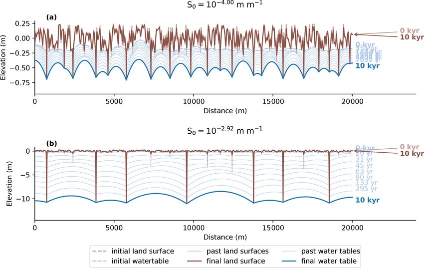
2                                                                            E. Luijendijk: Groundwater and drainage density

meability, groundwater flow and drainage density. However,
to my knowledge, a causal mechanism for this relation has
not been proposed.
   Most numerical landscape models use simplified repre-
sentations of groundwater flow and do not simulate the wa-
ter table or lateral groundwater flow directly (Tucker et al.,
2001a; Bogaart et al., 2003; van der Meij et al., 2018). There
are some exceptions, including two case studies of individ-
ual river catchments (Huang and Niemann, 2006; Barkwith
et al., 2015) and a generic model study (Zhang et al., 2016),
that concluded that the inclusion of groundwater flow has a
strong effect on modelled relief and erosion rates. Recently, a
groundwater flow component has been added to the Landlab           Figure 1. Conceptual model showing the hydrological and erosion
                                                                   process represented in the new model code. The hydrological pro-
landscape evolution model code (Litwin et al., 2020). How-
                                                                   cesses include groundwater flow, overland flow and streamflow. The
ever, to my knowledge, there has been no systematic model          erosion processes include hillslope diffusion and stream incision.
study to explore the relation between groundwater flow and
drainage density.
   Here, I present a new coupled model of groundwater              blue area. Saturation overland flow occurs where the ground-
flow, overland flow and erosion. The model was inspired by         water level is so close to the surface that there is no storage
the coupled groundwater and streamflow model of de Vries           space available in the unsaturated zone. Note that infiltration-
(1994). The model simulates lateral groundwater flow, the          excess overland flow is included in the model code but is
water table, and the water table’s effect on the partitioning      not used in this study because of the focus on humid re-
of groundwater and overland flow. The model also includes          gions, where infiltration-excess overland flow is of minor im-
erosion processes that follow widely used equations (Tucker        portance (Dunne, 1978; Bogaart et al., 2003). Groundwater
and Hancock, 2010). The model is used to explore the sensi-        flow and saturation overland flow contribute to steady-state
tivity of drainage density to parameters that govern ground-       and transient streamflow respectively. Both components of
water flow, streamflow and erosion. The focus is on humid          streamflow lead to erosion and incision of the stream. In ad-
regions where infiltration-excess overland flow is of minor        dition, the areas outside streams erode by hillslope diffusion,
importance and where the groundwater system is tightly cou-        which is a simplified representation of processes such as soil
pled with the surface water system. The results point to a         creep (Culling, 1960, 1963).
strong relation between drainage density, groundwater flow            The model starts with a rectangular model domain with a
and transmissivity. In addition, the results illustrate the pro-   constant slope in one direction. The rectangular model do-
cess of groundwater capture that explains this relation.           main contains a single cross section that is oriented perpen-
                                                                   dicularly to the slope and that is used to solve the groundwa-
2     Methods                                                      ter flow, overland flow and the hillslope diffusion equations.
                                                                   The initial topography in the direction of the cross section
2.1    Model description                                           is randomly perturbed. The topography evolves over time
                                                                   as a result of stream incision and hillslope diffusion. The
The model code described here simulates steady-state               model simulates groundwater flow, overland flow and hill-
groundwater flow, transient saturation overland flow, stream       slope diffusion in the 2D cross section. All streams are as-
incision and hillslope diffusion in a 2D cross section of          sumed to run perpendicular to the cross section and are per-
the subsurface. These processes are shown schematically in         fectly straight and parallel. Streamflow and stream incision
Fig. 1. The model code is named “the groundwater flow,             are calculated by multiplying the water and sediment flux in
overland flow and erosion model”, or GOEMod, and was               the 2D cross section by the contributing area perpendicular to
inspired by the conceptual groundwater outcrop erosion             the cross section. Thus, water and sediment transport in the
model originally presented by de Vries (1976) and sub-             out-of-plane direction take place in a series of perfectly par-
sequently implemented as a set of coupled analytical so-           allel streams that develop along an inclined topography. The
lutions for groundwater and streamflow (de Vries, 1994).           workflow and equations for each component of the model are
GOEMod is an open-source code and is available online on           discussed in detail in the following sections.
Zenodo (Luijendijk, 2021) and GitHub (https://github.com/
ElcoLuijendijk/goemod, last access: 3 November 2021).
                                                                   2.2   Initial topography
   Groundwater flow is approximated as steady state, with
the dark blue line in Fig. 1 showing the average groundwa-         The model starts with a random initial topography, which is
ter level. Each precipitation event adds a volume of water         calculated as using a series of 400 linear segments with ran-
on top of the average groundwater level, shown by the light        dom placement and random perturbation of the elevation at

Earth Surf. Dynam., 10, 1–22, 2022                                                      https://doi.org/10.5194/esurf-10-1-2022
E. Luijendijk: Groundwater and drainage density                                                                                      3

the start and end points of the segments. For the model sim-
ulations shown in this study, the average initial elevation is
0 m and the initial relief is 0.5 m.

2.3    Precipitation
Precipitation events are quantified using rainfall intensity
statistics for the Netherlands (Beersma et al., 2019), utilizing
a precipitation–frequency curve shown in Fig. 2. The rainfall
intensity curves follow a generalized extreme value distribu-
tion with the parameters given by the following equations
(Beersma et al., 2019):

η = 1.02(0.239 − 0.0250 log(D/60.))−1/0.512                 (1)
γ = 0.478 − 0.0681 log(D)                                   (2)    Figure 2. Precipitation–frequency curve for the Netherlands, fol-
                                                                   lowing Beersma et al. (2019), for precipitation events with a dura-
κ = 0.118 − 0.266 log(D) + 0.0586(log(D)2 ).                (3)    tion of 3 h. This curve was used to model precipitation, groundwater
                                                                   recharge and overland flow.
Here, η is the location parameter, γ is the dispersion param-
eter, κ is the shape parameter of the distribution and D is
the duration of each rainfall event (s). For the model exper-      domain, the available storage in the unsaturated zone is cal-
iments shown in this study, a rainfall duration (D) of 3 h is      culated using the depth of the water table and the specific
used. The precipitation depth for a single precipitation event     yield of the subsurface:
is calculated as follows:
                                                                   s = Sy (z − h),                                                 (6)
Pd = 1000.0η 1.0 + γ /κ(1.0 − T −κ ) ,

                                                           (4)
                                                                   where s is storage (m), Sy is specific yield (dimensionless), z
where Pd is the rainfall depth per event (m), and T is repe-       is the elevation of the land surface (m) and h is the elevation
tition time (a), which is the reciprocal of precipitation fre-     of the water table (m). Groundwater recharge for a single
quency f (a−1 ). The model simulates overland flow and             precipitation event is calculated as follows:
groundwater recharge for an average year. The total num-                 (
                                                                           s     if s < Pd
ber of precipitation events in a single year is found by adding    Ri =                      ,                                 (7)
up a series of precipitation events until the sum of the indi-             Pd if s>=Pd
vidual events matches a desired volume for the total annual        where Pd is the precipitation depth per event (m), and Ri is
precipitation (Pt ):                                               the groundwater recharge depth per event (m),
       i=f                                                            The time-averaged potential recharge rate Rp (m s−1 ) is
       X2
Pt =          (Pd (i)f (i)) .                               (5)    calculated as the sum of the individual recharge events as
       i=f1                                                        follows:
                                                                                       !
                                                                           i=n
   The precipitation events per year are calculated start-
                                                                           X
                                                                   Rp =        (Ri fi ) /1tr ,                              (8)
ing with a frequency (f1 ) of 1 a−1 . Subsequently, higher-                i=11
frequency (and lower-magnitude) events are added progres-
sively until the desired amount of total precipitation per year       where fi is the frequency of precipitation event i (s−1 ),
is reached. The precipitation statistics are based on an av-       and 1tr is the duration of the reference time period, which is
erage humid climate, such as the Netherlands, with a total         1 year (s). The actual recharge rate is calculate by subtracting
precipitation (Pt ) of 0.75 m a−1 .                                evapotranspiration:
                                                                        (
                                                                          Rp − ET if Rp > ET
2.4    Partitioning of groundwater and overland flow               R=                              ,                            (9)
                                                                          0           if Rp ≤ ET
The subdivision of precipitation between evapotranspiration,
overland flow and groundwater flow in the model is calcu-          where ET is the evapotranspiration rate (m s−1 ). Note that,
lated for individual precipitation events. For each precipi-       for simplicity, the evapotranspiration rate is assumed to be a
tation event, groundwater recharge is assumed to equal the         fixed value and independent of the depth of the water table.
available storage in the unsaturated zone (i.e. all groundwater       Saturation overland flow is calculated as the amount of
stored in the unsaturated zone is assumed to eventually per-       precipitation that exceeds the available storage (s) in the un-
colate to the groundwater table). For each point in the model      saturated zone. For each node in the model domain and for

https://doi.org/10.5194/esurf-10-1-2022                                                     Earth Surf. Dynam., 10, 1–22, 2022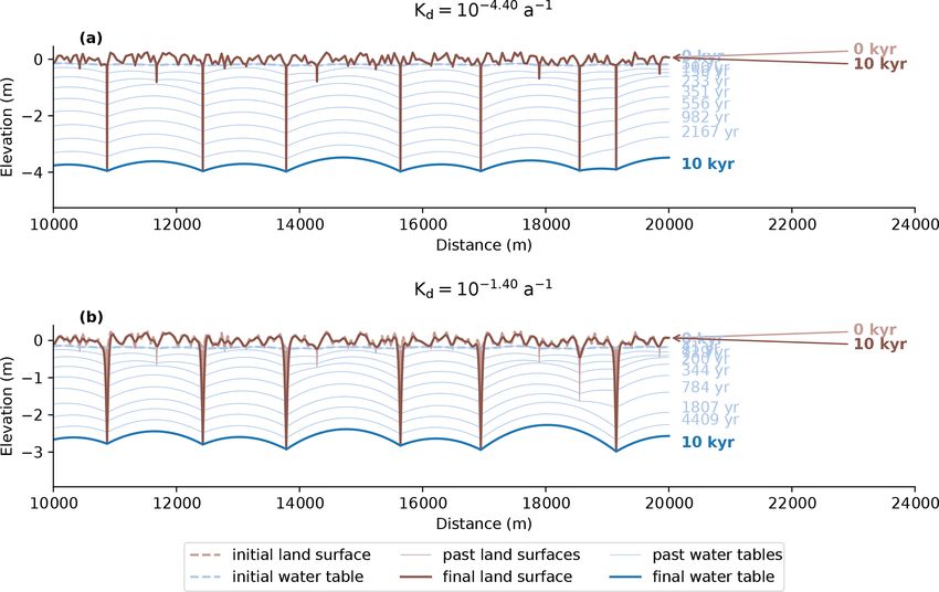
4                                                                             E. Luijendijk: Groundwater and drainage density

                                                                    where Re is the effective in-plane recharge (m s−1 ), and Lu
                                                                    is the length of the upstream contributing area (m).
                                                                       In-plane groundwater flow is calculated using the Dupuit–
                                                                    Forchheimer equation, which describes depth-integrated
                                                                    steady-state groundwater flow between two groundwater dis-
                                                                    charge points (Forchheimer, 1886; Bresciani et al., 2016):

                                                                           Re
                                                                    1h =      x(L − x) + 1H x/L,                               (13)
                                                                           2T
                                                                    where h is the hydraulic head (m), L is the distance between
                                                                    two groundwater discharge points (m), x is the distance to the
                                                                    first discharge point (m) and 1H is the difference in water
                                                                    level between the two discharge points (m). The term ground-
Figure 3. Calculated out-of-plane groundwater flow for a range      water discharge point represents a point such as a stream or a
of values of transmissivity and stream slope, using the base-case   part of the land surface where the water table is at the surface
values of the contributing area (5 km) and groundwater recharge     and where groundwater seepage takes place. The equation
(0.375 m a−1 ).                                                     assumes that the lateral differences in the hydraulic head (h)
                                                                    are much smaller than the thickness of the aquifer (Bresciani
                                                                    et al., 2016).
each precipitation event, the saturation overland flow depth
                                                                       For points at the edge of the model domain that are only
is calculated as follows:
                                                                    bound by a discharge point on one side, the equation reduces
                                                                    to
       (
         Pd − S if s < Pd
Qsi =                         ,                         (10)
         0         if s>=Pd                                                Re
                                                                    1h =      x(Lb − 0.5x),                                    (14)
                                                                           T
where Qsi is the saturation overland flow depth per precipi-
tation event (m).                                                   where Lb is the distance between the discharge point and the
                                                                    lateral model boundary (m). The average in-plane ground-
2.5   Groundwater flow                                              water recharge rate Re was calculated as the average effective
                                                                    recharge rate for all the nodes in between two seepage nodes.
The model is based on the assumption that groundwater flow          The seepage nodes represent points where the water table is
can be considered to be in steady state on the timescales of        at the surface and where groundwater discharge occurs. The
stream and hillslope erosion processes. This was judged to          position of the seepage nodes is not known in advance; in-
be reasonable because the groundwater flow system reacts            stead, it is calculated using the following iterative procedure:
much faster than the relatively slow rates of erosion. Given
these assumptions, groundwater flow and the position of the          1. First, one seepage node is picked at the lowest elevation
water table can be calculated using analytical solutions of             in the model domain, and the water table is calculated
steady-state groundwater flow.                                          using Eqs. (13) and (14). In most cases, the calculated
   First, the out-of-plane component of groundwater flow                water table is still above the land surface in a large part
(i.e. groundwater flow parallel to the direction of the nearest         of the model domain after the first iteration.
stream) is calculated using Darcy’s equation and assuming
that the out-of-plane hydraulic gradient is equal to the (out-       2. Subsequently, a new seepage node is added at the node
of-plane) slope of the nearest stream:                                  with the lowest elevation in the part of the model do-
                                                                        main where the modelled water table exceeds the land
Qgo = T S,                                                  (11)        surface.

where T is transmissivity (m2 s−1 ), and S is stream slope           3. The water table is recalculated using this new additional
(m m−1 ). Out-of-plane groundwater flow can be significant              seepage node.
for cases with high transmissivity or stream slope, as shown
in Fig. 3.                                                           4. The last two steps are repeated until the modelled water
   The remaining in-plane groundwater flow (i.e. towards the            table is below or at the land surface (i.e. h ≤ z) every-
nearest stream) is calculated using the value of recharge cal-          where.
culated in Eq. (8) and subtracting the out-of-plane discharge:
                                                                      An example of the calculated water table and seepage lo-
Re = RLu − Qgo ,                                            (12)    cations following the procedure is shown in Fig. 4.

Earth Surf. Dynam., 10, 1–22, 2022                                                      https://doi.org/10.5194/esurf-10-1-2022
E. Luijendijk: Groundwater and drainage density                                                                                      5

                                                                      Figure 5. Example of calculated baseflow to streams. The coloured
Figure 4. Example of initial topography and calculated water table    triangles denote the magnitude of the calculated baseflow.
and groundwater seepage locations. The water table and seepage
locations were calculated by an iterative solution of Eqs. (13) and
(14), as explained in Sect. 2.5.                                      2.6.2        Saturation overland flow
                                                                      The volume of water that is contributing to overland flow is
2.6     Streamflow
                                                                      calculated per precipitation event as follows:
                                                                              Zx2
The water flow in each stream consists of two components:
(1) steady baseflow supplied by groundwater discharge and             V0 =          Qsi dx,                                        (16)
(2) transient flow that consists of overland flow. The calcu-                 x1
lation of both components is described in the following two           where V0 is the volume of water to be discharged in a stream
sections.                                                             channel (m3 ), x1 and x2 are the positions of the topographic
                                                                      divide on either side of the channel (m), and Qsi is the rate of
2.6.1    Baseflow                                                     overland flow for each node as calculated using Eq. (10). An
The baseflow in each stream node is calculated in two steps.          example of the resulting distribution of precipitation excess
First, streams nodes are found by finding the node with the           and overland flow is shown in Fig. 6.
lowest elevation for each series of neighbouring seepage
nodes in the model domain. Note that the term seepage nodes           2.6.3        Water level in streams
is used here to denote nodes where groundwater discharge              The water level in streams as a result of baseflow and over-
occurs. The 2D (in-plane) value of groundwater flow toward            land flow is calculated using the Gauckler–Manning equa-
each stream node (qb ) is calculated for each stream by find-         tion for stream discharge. The Gauckler–Manning equation
ing the nodes contributing groundwater to each stream and             for stream discharge is as follows (Gauckler, 1867; Manning,
by summing the product of the recharge rate at each node              1891):
R and the width of each node (1x). The contributing area
is found by the taking the water table h as calculated using          v = Kn R 2/3 S 1/2 ,                                         (17)
Eqs. (13) and (14) and finding the two nodes on either side of
each stream where the hydraulic gradient changes direction.           where v is the mean flow velocity in a stream channel
The 3D (out-of-plane) value of baseflow was calculated by             (m s−1 ); Kn is an empirical coefficient (m1/3 s−1 ) that is de-
multiplying in-plane baseflow (qb ) by an upstream length of          fined as 1/n, where n is the Manning’s roughness coefficient
each stream:                                                          (s m−1/3 ); R is hydraulic radius (m); and S is the slope of the
                                                                      water surface, which is assumed to be equal to the slope of
Qb = qb Lu ,                                                  (15)    the channel bed (m m−1 ). With the common assumption that
                                                                      channels are much wider than they are deep, R ≈ hc and the
where Qb is baseflow. An example of the calculated value of           equation can be simplified to
baseflow is shown in Fig. 5.
                                                                                        2/3
                                                                      v = Kn S 1/2 hc ,                                            (18)

                                                                      where hc is the water height in the channel (m). The dis-
                                                                      charge is equal to the product of the flow velocity and the
                                                                      cross-sectional area. To simplify the equations the cross sec-
                                                                      tion for each stream is assumed to be triangular. The linear

https://doi.org/10.5194/esurf-10-1-2022                                                          Earth Surf. Dynam., 10, 1–22, 2022
6                                                                                    E. Luijendijk: Groundwater and drainage density

                                                                         prohibitive computational expensive. Instead, this work de-
                                                                         rives new equations for the total discharge in a stream follow-
                                                                         ing a single precipitation event. To keep the solution math-
                                                                         ematically tractable, the assumption is made that each pre-
                                                                         cipitation event generates a volume of overland flow that is
                                                                         added instantaneously to the stream channel. The volume is
                                                                         subsequently discharged over time.
                                                                            The continuity equation for discharge of a stream channel
                                                                         is given by

                                                                         ∂Vw
                                                                             = −Qw ,                                                (21)
                                                                          ∂t

                                                                         where Vw is the water volume in the channel (m3 ). The vol-
                                                                         ume to be discharged is defined as the product of a cross-
                                                                         sectional area that changes over time and a fixed stream
                                                                         length Lu (m):

                                                                         Vw = ALu .                                                 (22)

                                                                         Assuming that the shape of the channel is a triangle and com-
                                                                         bination with the stream discharge equation (Eq. 19) yields

                                                                         Lu ∂h2c    Kn S 1/2 8/3
Figure 6. Example of calculated precipitation excess and saturation
                                                                                 =−         hc .                                    (23)
                                                                         St ∂t        St
overland flow in streams. Panel (a) shows the calculated precipita-
tion excess for each node in the model domain. Panel (b) shows the         Integration of this equation with boundary condition hc =
location of nodes where the precipitation depth for a single event       h0 at t = 0 yields
exceeds the available storage, which results in fully saturated condi-
tions and the generation of saturation overland flow. Panel (c) shows                            −3/2
                                                                                      Kn S 1/2

the calculated saturation overland flow volume for each stream in              −2/3
                                                                         hc = h0    +          t       .                            (24)
the model domain. Note that all of the potential streams are shown                     3L
here, including potential streams in depressions that do not generate
overland flow because they are located too far above the water table.       The initial height of the water level in the channel (h0 ) is
                                                                         related to the initial volume of water in the channel V0 :

in-plane slope of the channel bed (i.e. perpendicular to the                    h20 Lu
                                                                         V0 =          .                                            (25)
flow direction in the channel) is denoted as St (m m−1 ). The                     St
cross-sectional area of the channel equals St h2 . Using this,
the discharge equation can be written as follows:                           Adding Eq. (25) into Eq. (24) and replacing the constants
                                                                         yields an expression for the decrease in the water level in a
        Kn S 1/2 8/3                                                     channel over time in response to the drainage of an initial
Qw =            hc ,                                             (19)    volume V0 :
          St
                                                                                                         !−3/2
where Qw is the discharge in the channel (m3 s−1 ). Rewrit-                      V0 St −1/3 Kn S 1/2
                                                                         hc =              +         t           .                  (26)
ing this equation yields an expression for the water level in                     Lu         3Lu
streams as a function of discharge:
                        3/8                                               This equation was validated by comparison with a numer-
            St Q w                                                       ical solution for the water level over time (Fig. 7). The nu-
hc =                 .          .                                (20)
            Kn S 1/2                                                     merical solution was calculated using the discharge equation
                                                                         (Eq. 19) to calculate discharge over time. At the first time
2.6.4       Transient stream discharge                                   step, the initial overland flow volume V0 is added. Subse-
                                                                         quently, discharge is calculated and subtracted from the ini-
The discharge generated by overland flow operates on short               tial volume V0 . The height of the water level at each time step
timescales of hours to days. Modelling this process directly             was calculated using Eq. (25). This process is repeated until
would require short time steps that would make the model                 the water level is less than 1 mm.

Earth Surf. Dynam., 10, 1–22, 2022                                                           https://doi.org/10.5194/esurf-10-1-2022
E. Luijendijk: Groundwater and drainage density                                                                                        7

                                                                         2.7.1   Base-level change
                                                                         The incision of streams results in an adjustment of the stream
                                                                         slope (S). The stream slope is also dependent on changes in
                                                                         the base level. The base level at the downstream boundary of
                                                                         the model domain is calculated as follows:
                                                                         zb = zb,0 + U t,                                           (28)
                                                                         where zb is the elevation of the downstream model boundary
                                                                         (m), U is the base-level change rate (m s−1 ) and t is the total
                                                                         elapsed time since the start of the model run (s). zb,0 (m)
                                                                         is the initial base level at the start of the model run and is
                                                                         calculated as the product of initial stream slope and distance
                                                                         to the downstream model boundary:
                                                                         zb,0 = z0 + S0 Ld .                                        (29)
                                                                         Here, z0 is the average elevation in the cross section at t = 0
                                                                         (m), which is 0 m for the model runs shown in this study;
                                                                         S0 is the initial slope (m m−1 ); and Ld is the distance to the
                                                                         downstream model boundary (m).
                                                                            After each time step, a new value of stream slope is calcu-
                                                                         lated using the new elevation of the base of the stream and
Figure 7. Validation of the equation for the transient discharge of an
                                                                         the elevation of the downstream edge of the model domain:
instantaneously added volume of water in a stream channel (Eq. 26)
using the numerical solution as described in the text. Panel (a)              zs − zb
                                                                         S=           ,                                             (30)
shows that the numerical solution and analytical solution overlap               Ld
perfectly. Panels (b) and (c) show the change in water volume and
                                                                         where zs is the elevation of the stream in the modelled cross
discharge in the channel over time, which were used to calculate the
numerical solution in panel (a). The solution uses the base-case pa-     section (m).
rameters listed in Table 1; a precipitation depth of 0.0365 m, which
is the theoretical maximum 1 d precipitation depth for a return time     2.7.2   Stream incision by baseflow
of 1 year for the Netherlands; and a contributing area for overland
flow with a length of 100 m.                                             The sediment flux in the steam channel carried by baseflow
                                                                         is calculated using Eq. (27), with the value of baseflow cal-
                                                                         culated using Eq. (15) as the value for water discharge Qw .
                                                                         The incision of the stream is calculated by dividing the sedi-
2.7   Stream incision
                                                                         ment flux by the channel width (w). In addition, the erosion
The sediment flux in a stream channel at carrying capacity               is divided over the upstream length of the stream by assum-
is given by the following equation (Tucker and Bras, 1998;               ing that erosion increases linearly from zero at the start of
Tucker and Hancock, 2010):                                               the stream to the maximum value at the end of the stream.
                                                                         This yields the following equation for erosion of the stream
                                                                         channel:
Qs = wkf (Qw /w)m S n ,                                          (27)
                                                                         ∂z              Qs
                                                                             = (1 − φ) 1 ,                                         (31)
                                                                          ∂t           w 2 Lu
where Qs is the sediment flux (m3 s−1 ), w is channel width
(m), kf is the sediment transport coefficient (s4/5 m−8/5 ),             where z is the elevation of the base of the channel (m), t
Qw is water discharge (m−3 s−1 ) and S is channel slope (di-             is time (s) and φ is porosity (dimensionless). Note that the
mensionless); m and n are the respective discharge exponent              linear increase in erosion by baseflow along the stream is a
(dimensionless) and slope exponent (dimensionless), which                simplification that makes the problem more tractable mathe-
were set to values of 1.8 and 2.1 respectively. The erosion by           matically. In reality, the non-linear relation between stream-
streams is subdivided into two components: (1) the erosion               flow and erosion would result in a non-linear increase in ero-
by baseflow driven by groundwater discharge and (2) the ad-              sion along the stream profile. Channel width was calculated
ditional transient erosion by saturation overland flow during            as follows (Lacey, 1930):
and directly after precipitation events. In addition, incision
                                                                         w = kw Qω ,                                                (32)
and stream slope are governed by the base level. The equa-
tions for the calculation of the base level and the two erosion          where kw and ω are empirical parameters that are set to val-
components are discussed in the following sections.                      ues of 3.65 and 0.5 respectively (van den Berg, 1995).

https://doi.org/10.5194/esurf-10-1-2022                                                          Earth Surf. Dynam., 10, 1–22, 2022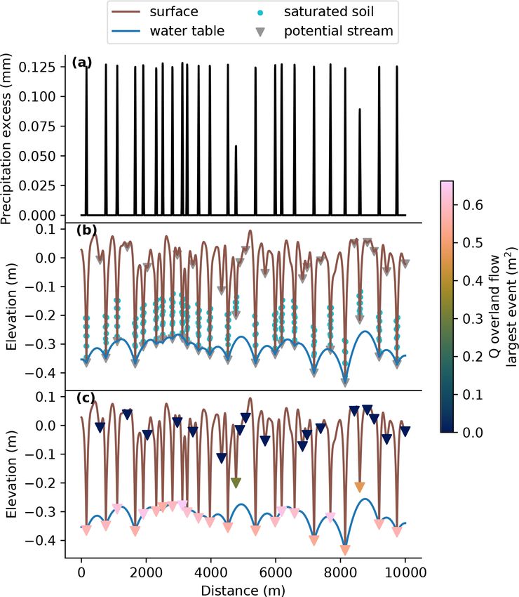
8                                                                              E. Luijendijk: Groundwater and drainage density

2.7.3     Stream incision by overland flow                          2.9    Iterative solution
Erosion by streams caused by the discharge of overland flow         The solution of the equations for groundwater flow, overland
is calculated by combining the equation for stream discharge        flow, streamflow and erosion follow an iterative scheme that
due to overland flow over time (Eq. 26) with the sediment           is detailed in Fig. 8. After setting up an initial topography,
discharge equation (Eq. 27). The combination of these two           the initial water table is calculated using the procedure de-
equations yields                                                    scribed in Sect. 2.5, with recharge taken as the difference be-
                                                      !−4m          tween the total precipitation (Pt ), overland flow and evapo-

               K   S 1/2 m  V S −1/3   K   S 1/2
Qs = k f S n
                 n             0  t
                                        +
                                            n
                                                    t      . (33)   transpiration (ET). Subsequently, the model calculates base-
                  St           Lu          3Lu                      flow, stream incision due to baseflow and overland flow, and
                                                                    topography change due to hillslope diffusion. Overland flow
  Integrating this equation from t = 0 to t = ∞ yields an
                                                                    and recharge are calculated on an event basis. Recharge is
expression for the total volume of sediment eroded from the
                                                                    summed over a year in order to yield an average recharge
channel after a single precipitation and discharge event:
                                                                    rate. Overland flow and erosion are calculated on an event
        a(b + c)(−4m+1)                                             basis and are then summed over a year in order to yield an av-
Vs =                    ,                                   (34)    erage overland flow erosion rate. This procedure is repeated
            4mc + c
                                                                    at each time step. The initial time step size is 1 year. The time
where Vs is the total volume eroded in a stream by overland
                                                                    step size was adjusted so that the maximum elevation change
flow following a single precipitation event, and a, b and c are
                                                                    per time step was 0.5 % of the total relief with a minimum of
constants that are defined as
                                                                    0.01 m. These conditions were found by trial and error to en-
                 1/2 m
         n Kn S                                                     sure numerically stable and computationally efficient model
a = kf S                                                   (35)
               St                                                   runs for the range of parameter values and runs reported in
                                                                    this study.
      V0 St −1/3

b=                                                         (36)
       Lu
                                                                    2.10    Base-case parameter values
   Kn S 1/2
c=          .                                               (37)    The base-case parameter values follow de Vries (1994) and
    3Lu
                                                                    Bogaart et al. (2003), who modelled stream network and
   The eroded volume results in incision of the stream.
                                                                    landscape evolution of the southern Netherlands under alter-
Stream incision by overland flow is calculated by distributing
                                                                    nating glacial and interglacial conditions. Here, the param-
the eroded volume (Vs ) evenly over the width of the stream
                                                                    eters that represent present-day (interglacial) conditions are
channel (w). In addition, erosion by overland flow is assumed
                                                                    used. The base-case parameters are listed in Table 1. In con-
to increase linearly from the start of the channel to the posi-
                                                                    trast to the relatively high value for porosity of 0.4 used by
tion of the modelled cross section. This is a similar simplifi-
                                                                    Bogaart et al. (2003), a value of 0.2 is used here, which more
cation to the linear increase in erosion by baseflow discussed
                                                                    closely follows values observed in areas covered by fluvial
in the previous section, and it was also used to keep the prob-
                                                                    and aeolian sediments in the southern Netherlands (de Vries,
lem mathematically tractable. This yields the following ex-
                                                                    1994). The base-case value for transmissivity is 1 × 10⁻²
pression for the incision of the stream due to overland flow:
                                                                    m2 s−1 , which is based on values that range from 0.012 to
            Vs                                                      0.03 m2 s−1 reported by de Vries (1994). The initial slope
1zs =                 ,                                     (38)
         (w 12 Lu )                                                 value of 5 × 10⁻⁴ m m−1 is equal to the average stream gra-
                                                                    dient in the southern Netherlands.
where 1zs is stream incision following a single precipitation          The value of the sediment transport coefficient reported by
event (m).                                                          Bogaart et al. (2003) was based on the theoretical Einstein–
                                                                    Brown equation. Here, the value of this parameter is based on
2.8     Hillslope diffusion                                         an analysis of alluvial sediment discharge data by Brownlie
Erosion of the parts of the model domain outside of the             (1981), as reported by Lammers and Bledsoe (2018). Follow-
streams follows the hillslope diffusion equation (Culling,          ing the sediment discharge equation (Eq. 27), the sediment
1960):                                                              transport coefficient (kf ) can be expressed as

∂z ∂ Kd ∂x  ∂z
                                                                           qs
    =            ,                                    (39)          kf =          .                                             (40)
∂t       ∂x                                                                qw S n
                                                                            m

where Kd is the hillslope diffusion coefficient (m2 s−1 ). This       The compilation of total sediment discharge from flume
equation was solved numerically with a standard implicit fi-        experiments and field observations by Brownlie (1981), as
nite difference approach using a matrix solver implemented          reported by Lammers and Bledsoe (2018), contains n = 1463
in the NumPy Python module (Harris et al., 2020).                   data points for which sediment discharge (qs ), water dis-

Earth Surf. Dynam., 10, 1–22, 2022                                                       https://doi.org/10.5194/esurf-10-1-2022
E. Luijendijk: Groundwater and drainage density                                                                                              9

Figure 8. Flow chart for the iterative solution of the groundwater flow, overland flow and erosion equations.

charge (qw ) and stream slope (S) are known. Following Bo-
gaart et al. (2003), the coefficients n and m are set to val-
ues of 1.8 and 2.1 respectively. Inserting these values into
Eq. (40) allows kf to be calculated for each of the 1463 data
points. The calculated distribution of kf using Eq. (40) is
shown in Fig. 9. Comparison of the measured sediment dis-
charge values and the denominator (qwm S n ) in Eq. (40) shows
that there is a reasonable correlation of the term qwm S n with
the sediment discharge rate. When using the median value
of kf = 103.1 to predict sediment discharge, the coefficient
of determination for log-transformed values of sediment dis-             Figure 9. Comparison of measured sediment discharge and the
                                                                                                   m S n in the sediment discharge equations
charge equals 0.62. The median value of kf = 103.1 was used              water discharge term qw
as the base-case parameter value for the model experiments               (Eqs. 27 and 40) (a) and the calculated variation of the sedi-
shown in this study. Note that more complex sediment trans-              ment transport coefficient (b) in a compilation of 1463 sediment
port equations that consider sediment grain size and trans-              discharge data from flume experiments and field observations by
                                                                         Brownlie (1981), as reported by Lammers and Bledsoe (2018). The
port thresholds yield a closer fit to the data (Lammers and
                                                                         lines in panels (a) and (b) denote the 0.05, 0.5 and 0.95 quantiles of
Bledsoe, 2018). However, these equations were not imple-
                                                                         the distribution of kf as calculated using Eq. (40).
mented in this study to keep the calculation of sediment dis-
charge for individual discharge events (Eq. 34) mathemati-
cally tractable.
                                                                         fusion coefficient (Kd ), sediment transport coefficient (kf )
2.11   Model sensitivity analyses                                        and base-level change (U). These values are listed in Table 2.
                                                                            The range of variation in the hillslope diffusion coefficient
To explore the role of groundwater flow in erosion, a series             was based on Richardson et al. (2019). There is no large com-
of model experiments were conducted with different values                pilation of transmissivity data available. Models and data of
for transmissivity and specific yield. To compare the effects            the permeability of unconsolidated sediments (Gleeson et al.,
of changes in groundwater flow with climate and erosion                  2011; Luijendijk and Gleeson, 2015) and a hydrologically
parameters, an additional set of experiments was conducted               active layer of approximately 100 m (Gleeson et al., 2016;
with different values for total precipitation (Pt ), hillslope dif-      Jasechko et al., 2017) suggest a variation of approximately

https://doi.org/10.5194/esurf-10-1-2022                                                            Earth Surf. Dynam., 10, 1–22, 2022
10                                                                                    E. Luijendijk: Groundwater and drainage density

Table 1. Base-case parameter values.

     Parameter group        Parameter name                    Symbol   Value               Reference
     Model geometry         Length                            L        20 000 m
                            Upstream length                   Lu       10 000 m
                            Downstream length                 Ld       10 000 m
                            Grid cell size                    1x       5m
     Relief                 Initial relief                             0.5 m
     Precipitation and ET   Precipitation event duration      D        1.0 d
                            Annual precipitation              P        0.75 m a−1          Bogaart et al. (2003)
                            Potential ET                      ET       0.375 m a−1         Bogaart et al. (2003)
     Streamflow             Channel roughness factor          Kn       25                  de Vries (1994)
                            Initial channel slope             S0       4 × 10⁻⁴            de Vries (1994)
                            Perpendicular channel slope       St       0.002               de Vries (1994)
                            Channel width coefficient 1       kw       3.65                van den Berg (1995)
                            Channel width coefficient 2       ω        0.5                 van den Berg (1995)
     Groundwater flow       Specific yield                    Sy       0.2                 de Vries (1994)
                            Transmissivity                    T        1 × 10⁻² m2 s−1     de Vries (1994)
     Erosion                Base-level change                 U        −10−5 m a−1         Bogaart et al. (2003)
                            Sediment transport coefficient    kf       103.1 s4/5 m−8/5    Brownlie (1981) and Lammers and Bledsoe (2018)
                            Discharge exponent                m        1.8                 Bogaart et al. (2003)
                            Slope exponent                    n        2.1                 Bogaart et al. (2003)
                            Hillslope diffusion coefficient   Kd       0.01 m2 a−1         Bogaart et al. (2003)
                            Porosity                          φ        0.2

10−7 to 10−1 m2 s−1 . Here, a smaller range of values is eval-             3     Results
uated (10−4 to 10−1 m) because, for the relatively low-relief
landscape that was studied, lower values of transmissivity                 3.1    Groundwater capture
result in drainage densities that are fully controlled by the
initial random topography. The values of specific yield are                Figure 10 shows the result of an example model run using the
based on values reported for mixed sediments (Revil, 2002;                 base-case parameter values as shown in Table 1. The figure
Gleeson et al., 2014; El-husseiny, 2020). The minimum and                  shows the evolution of the land surface from an initial ran-
maximum values for the sediment transport coefficient were                 domly generated surface over a time span of 10 000 years.
equal to the 0.05 and 0.95 quantiles of the calculated distri-             The system starts out with a very high drainage density, with
bution of kf shown in Fig. 9.                                              114 streams in a model domain that is 20 km long. Subse-
                                                                           quently, the model evolves rapidly towards a system domi-
                                                                           nated by fewer streams over time, with the final number of
2.12     Additional model experiments                                      12 active streams after a runtime of 10 000 years.
                                                                              The decrease in number of streams is caused by a pro-
In addition to the model sensitivity analysis, a second set of             cess that is defined here as groundwater capture, by which
model experiments was conducted to explore the persistence                 faster eroding streams draw the water table below neighbour-
of drainage density over longer timescales. These model ex-                ing streams and reduce the baseflow and saturation overland
periments used the modelled incised topography of the base-                flow of these streams until they become dry. The process of
case model run after 10 000 years as a starting point and sub-             groundwater catchment capture is illustrated in more detail in
sequently added another 50 000 years to the simulation, al-                Fig. 11, which shows the land surface, water table and stream
though with different parameter values that follow the sensi-              fluxes for three time slices before, during and after a ground-
tivity analysis reported in the previous section and Table 2.              water catchment capture event. After 2251 kyr (Fig. 11a), 13
These different parameter values resulted in model simula-                 streams are still active. However, the last stream on the right-
tions where the system was out of balance with the incised                 hand side has a smaller catchment area and a lower baseflow
topography. The degree to which these runs resulted in an                  and, therefore, incises slower than its neighbouring stream.
adjustment of the stream network and drainage density after                After 2457 years (Fig. 11b), the neighbouring stream has in-
a runtime of 10 000 and 50 000 years was recorded and used                 cised further and has drawn the water table below the base of
to quantify the persistence of stream networks.                            the stream. The stream does generate overland flow but has

Earth Surf. Dynam., 10, 1–22, 2022                                                               https://doi.org/10.5194/esurf-10-1-2022
E. Luijendijk: Groundwater and drainage density 11
Table 2. Parameter value range in model sensitivity analyses.
Parameter name Symbol Minimum Maximum Number of
value value steps
Precipitation P 0.5 m a−1 1.5 m a−1 10
Transmissivity T 1 × 10⁻⁵ m 1 × 10⁻¹ m 10
Specific yield Sy 0.15 0.5 10
Hillslope diffusion coefficient Kd 4 × 10⁻⁵ m2 a−1 4 × 10⁻² m2 a−1 10
Sediment transport coefficient kf 102.3 s4/5 m−8/5 104.2 s4/5 m−8/5 10
Base-level change U 10−5 m a−1 10−3 m a−1 10
ceased to generate baseflow. At 2707 years, the water table 3.2 Sensitivity of drainage density to transmissivity
has been drawn down further and is too deep for the stream to
generate saturation overland flow (i.e. all of the precipitation Groundwater capture is dependent on the transmissivity of
that falls near the stream can be accommodated in the unsatu- the subsurface. This is illustrated by three model runs with
rated zone above the water table). As a result, the stream has different values of transmissivity (Fig. 13). The model run
become inactive. The stream channel has partly been filled with the lowest transmissivity shows the highest drainage
by hillslope diffusion, as the sediment flux caused by hills- density (Fig. 13a), and the model run with a highest value
lope diffusion is no longer compensated for by the removal of transmissivity shows the lowest value of drainage den-
of sediment by streamflow. sity (Fig. 13c). The reason for this is that low transmissiv-
The evolution of the stream network over time is summa- ity results in higher water table gradients, which makes it
rized in Fig. 12. Initially, each small depression is potentially much more difficult for streams to draw the water table be-
an active stream channel, which results in a large number low neighbouring streams and to capture their groundwater
of active streams. However, as the incision of streams in- discharge. In contrast, high transmissivity results in a rela-
creases, the number of active streams drops rapidly in the tively flat water table, which means that small differences in
first 100 years, followed by a slower reduction in the number incision can already lead to a water table that is drawn be-
of active streams. The last stream capture event at 2457 years low the base of streams. There is a small positive correlation
is shown in Fig. 11. After this event, the drainage system re- between transmissivity and stream incision rate. The lower
mains in a steady state. Note that the model runtime in Fig. 12 number of streams at high values of transmissivity means
was extended to 1 million years to show the evolution of the that these streams receive more water and, therefore, have
landscape and stream network over a long time span. a higher erosion power. This effect is limited by the nega-
The initially high rate of groundwater capture is slowed tive feedback on stream incision that results from a decrease
down over time by the negative feedback imposed by the base in stream slope between the modelled cross section and the
level at the downstream (out-of-plane) end of the model do- base level at the downstream (out-of-plane) end of the model
main. The stream slope is lower for streams that have incised domain. For streams with a higher rate of incision, the slope
deeper, which limits their incision power. The negative feed- is reduced and their erosional power is decreased.
back on incision results in the establishment of a steady-state
drainage network after 2500 years. For the base-case model 3.3 Sensitivity of drainage density to hydrological and
run shown in Fig. 10, the base level is located at an elevation erosion parameters
of −4 m, at a downstream distance of 10 000 m.
The incision and the reduction of active streams by Comparison of drainage density and incision to a number
groundwater capture also means that the area susceptible to of parameters that govern erosion and streamflow show that
saturation overland flow decreases over time, as saturation drainage density is the most sensitive to transmissivity and
overland flow takes place near active stream channels where initial slope (Fig. 14). Drainage density is also affected by
the water table is located close to the surface. Apart from precipitation and base-level change, whereas it is largely in-
a short phase at the start of the model run, streamflow and sensitive to specific yield, the sediment transport coefficient
stream erosion are predominantly generated by groundwater and the hillslope diffusion coefficient.
flow, which is referred to as baseflow once it enters the stream The strong negative correlation of drainage density and
channel (Fig. 12b, c). initial downstream slope is illustrated in Fig. 15 and can be
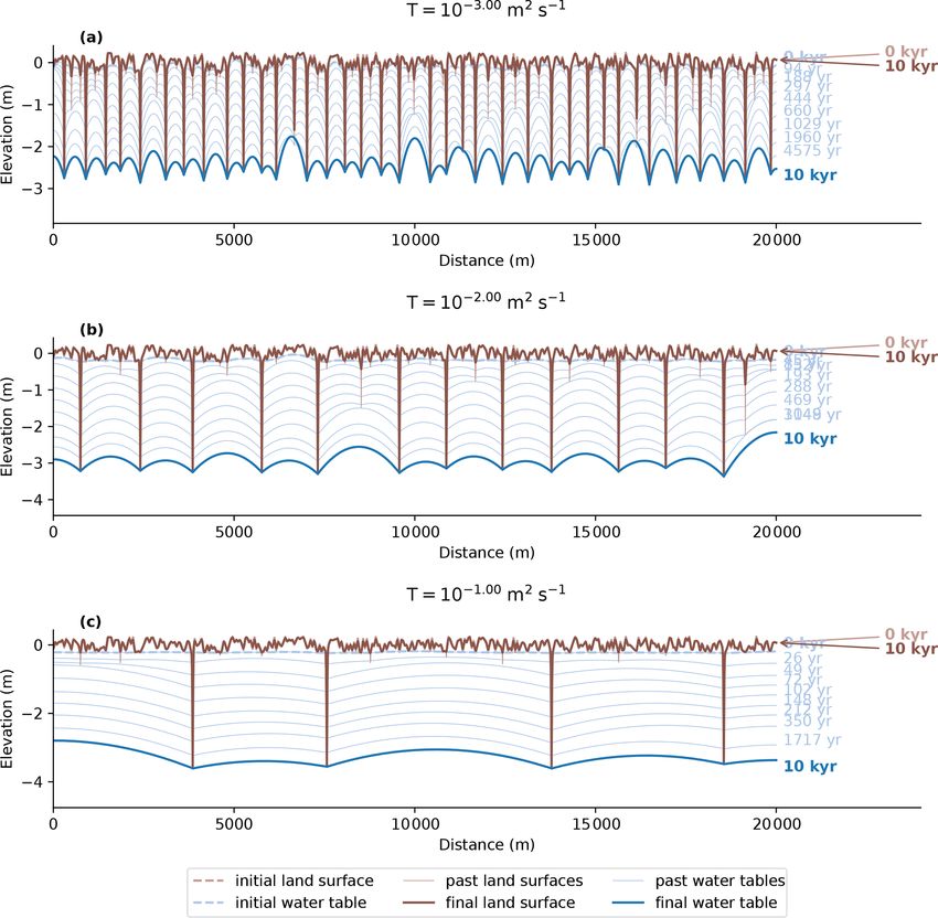
explained by three effects. First, a higher stream slope means
that individual streams have a higher incision power, which
means that it is easier to draw the water table below adjacent
streams and capture their groundwater discharge. Second, a
higher stream slope means a lower base level at the down-
https://doi.org/10.5194/esurf-10-1-2022 Earth Surf. Dynam., 10, 1–22, 202212 E. Luijendijk: Groundwater and drainage density Figure 10. Modelled change in the land surface and water table over 10 000 years for the base-case model run. The results show the evolution from a random topography with a high number of streams to an incised topography with 12 active streams. The past positions of the land surface and water table show the decrease in the number of streams over time. Figure 11. Illustration of groundwater capture in the base-case model run. Panels (a), (b) and (c) show modelled streamflow generated by baseflow and overland flow, and the change in elevation caused by hillslope diffusion and stream erosion for three time slices before, during and after a capture event respectively. Panels (d), (e) and (f) show the modelled position of the land surface and the water table during these three time slices. The arrow points to the stream that loses its connection with the groundwater table. stream end of the model domain, which means that streams high drainage densities and vice versa. However, at low pre- can incise deeper and capture more adjacent streams before cipitation values, this trend is reversed, as all recharge con- the negative feedback kicks in that is associated with deep in- tributes to out-of-plane groundwater flow, and the in-plane cision and a reduction in stream slope. Third, a higher initial groundwater flow, baseflow and overland flow rates are too downstream slope means that more of the total groundwa- low for the streams to incise. This means that the initially ter recharge is directed downstream in the out-of-plane di- high number of streams does not decrease over time. rection, and there is less in-plane groundwater flow (Fig. 3). Specific yield only has a subtle effect on stream incision. This results in flatter water tables and an increase in ground- Lower values of specific yield increase the volume of satu- water capture. ration overland flow and make it more difficult for streams Precipitation shows a complex relation with drainage den- to run completely dry, even if they are disconnected from the sity (Fig. 14), with a positive correlation between drainage water table. However, given the subordinate importance of density and precipitation at moderate to high values of pre- overland flow in generating streamflow and erosion in these cipitation, but very high drainage density and low incision model experiments, this effect is very modest and does not rates at low values of precipitation. Precipitation affects change the modelled drainage density or incision rate after a groundwater recharge. Given that groundwater flow depends model runtime of 10 000 years (Fig. 14). on the ratio of recharge over transmissivity (see Eq. 13), The sediment transport coefficient exerts a strong control recharge has an effect of equal magnitude to that of transmis- on the rate of incision and controls how fast the drainage net- sivity but is opposite with respect to the direction of the ef- work reaches a steady state. High sediment transport coef- fect; in other words, high precipitation and recharge result in ficients result in high rates of incision and a relatively fast Earth Surf. Dynam., 10, 1–22, 2022 https://doi.org/10.5194/esurf-10-1-2022
E. Luijendijk: Groundwater and drainage density                                                                                     13

                                                                       3.4   The persistence of stream networks

                                                                       The model runs shown up until this point all started with flat
                                                                       topography with a random perturbation of ±0.5 m. However,
                                                                       the current drainage network in most natural systems started
                                                                       out on an older network that was, for instance, adjusted to
                                                                       glacial conditions during the Pleistocene. The effect of exist-
                                                                       ing incised topography on the modelled adjustment of stream
                                                                       networks is shown in Figs. 17 and 18.
                                                                          Figures 17 shows the change in the stream network fol-
                                                                       lowing a change in slope and base level. The results indi-
                                                                       cate that pre-existing incised topography delays the evolution
                                                                       of stream networks to higher drainage densities, whereas an
                                                                       evolution to lower drainage density proceeds more rapidly.
                                                                       A decrease in slope S0 from the base-case value of 4 ×
                                                                       10−4 to 1 × 10⁻⁴ m m−1 leads to a decrease in incision over
                                                                       time. However, the effect on drainage density is limited.
                                                                       The drainage density is increased only after approximately
                                                                       9000 years when the decrease in incision has progressed
                                                                       far enough that the water table reconnects with a previ-
                                                                       ously abandoned stream channel on the right-hand side of the
                                                                       model domain (Fig. 17a). This demonstrates that the stream
                                                                       network shows a degree of delay in adjustment to new con-
                                                                       ditions that depends on the depth of the water table and the
                                                                       ability of the water table to reconnect with abandoned stream
Figure 12. Changes in drainage density (a), water discharge (b),       channels or depressions in the landscape. Conversely, an in-
sediment flux (c), and elevation and relief (d) over a time span of    crease in slope leads to an increase in incision that allows
1 million years for the base-case model run. The results show a de-    the process of drainage capture to proceed (Fig. 17b). Differ-
crease in active stream channels and a decrease in saturation-excess   ences in catchment size lead to differences in incision rates
overland flow over time as streams incise and the water table is       and the capture of the groundwater discharge of several small
drawn deeper below the land surface.                                   streams by neighbouring streams. This results in a reduction
                                                                       in active streams over time from 12 to 7.
                                                                          The asymmetry in the response of the drainage network
adjustment of the stream network. However, the rate of inci-           to parameter changes is also shown in the model sensitiv-
sion is ultimately limited by the base level at the downstream         ity analyses presented in Fig. 18. Compared with model runs
end of the model domain, as explained previously; as a result,         that start with a flat topography (Fig. 18a), the model runs
the sediment transport coefficient only has a minor effect on          that started with an incised topography (Fig. 18b, c) show
the modelled drainage density (Fig. 14).                               a comparable response when the parameter change leads
   The effect of changes in the hillslope diffusion rate on the        to a reduction in drainage density. However, an increase in
development of streams is illustrated in Fig. 16. Although             drainage density is much harder to accomplish, as an in-
hillslope diffusion may be important in determining drainage           crease in drainage density is only possible when the water
density in landscapes with higher relief (Tucker and Bras,             table is close to the surface. For systems where incision has
1998; Perron et al., 2008), the incision power of streams is           progressed far enough for the water table to be well below the
high enough to outpace sediment delivery by hillslope dif-             surface, this requires large changes in precipitation or a large
fusion in this case, and the sensitivity analysis shows no ef-         decrease in incision. The adjustment of incision also means
fect of hillslope diffusion on drainage density (Fig. 14). The         that the time that has elapsed since a parameter change is
results do show an effect on the lateral slope of stream val-          important for drainage density. The delay in adjustment af-
leys and on the rate of infilling of abandoned stream channels         fects models after a runtime of 10 000 years (Fig. 18b) but is
(Fig. 16).                                                             much less important for model runs that last 50 000 years
                                                                       (Fig. 18c). The exception is formed by changes in trans-
                                                                       missivity, for which the effect is strong enough to generate
                                                                       a fast response in both directions (i.e. for both an increase
                                                                       and decrease in drainage density). However, abrupt changes
                                                                       in transmissivity are probably somewhat unlikely in reality.
                                                                       They could occur for areas with a gain or loss of permafrost

https://doi.org/10.5194/esurf-10-1-2022                                                        Earth Surf. Dynam., 10, 1–22, 2022
14 E. Luijendijk: Groundwater and drainage density
Figure 13. Modelled change in the land surface and water table over time for three model experiments with low (T = 10−3 m2 s−1 , panel a),
moderate (T = 10−2 m2 s−1 , panel b) and high (T = 10−1 m2 s−1 , panel c) transmissivity. The results show a negative correlation be-
tween drainage density and transmissivity and a positive correlation between transmissivity and stream incision over the model runtime of
10 000 years.
(Bogaart et al., 2003), or in the case of the erosion of a con- highly simplified distribution of the eroded volume over the
fining layer that shields a more permeable layer. length of the channel.
In spite of these limitations, the conclusions of the impor-
tance of groundwater flow for drainage density and stream in-
4 Discussion
cision are arguably relatively robust. The model results show
that groundwater capture is a somewhat inevitable conse-
quence of coupling groundwater flow, streamflow and ero-
4.1 Limitations of the model code
sion equations. Regardless of the exact equations and numer-
The model code presented here was intentionally kept as sim- ical implementation used, the water table will always crop
ple as possible to keep the solutions mathematically tractable out at perennial streams, and the incision of these streams
and the computational effort manageable. The main limita- will draw the water table down. Thus, smaller streams losing
tions are that the model is 2D and only represents a sys- their groundwater discharge and eventually falling dry is a
tem with perfectly parallel and straight streams; groundwa- logical consequence of differences in incision rate between
ter flow is in a steady state and the contribution of transient streams. These conclusions are also supported by previous
groundwater discharge or subsurface storm flow to stream- model studies that found that groundwater flow had a strong
flow is neglected; and the treatment of erosion by overland effect on erosion (de Vries, 1994; Huang and Niemann, 2006;
flow is highly simplified, with an instant addition of all over- Barkwith et al., 2015; Zhang et al., 2016) and that a corre-
land flow to the nearest active stream channel as well as a lation exists between permeability, transmissivity, or lithol-
Earth Surf. Dynam., 10, 1–22, 2022 https://doi.org/10.5194/esurf-10-1-2022E. Luijendijk: Groundwater and drainage density 15 Figure 14. Sensitivity of drainage density and stream incision to hydrological and erosion parameters. The incision rate denotes the incision rate of the stream with the lowest elevation at the end of each model run. Note that the range of parameter values reflects their variability in humid and subhumid settings, as explained in the text. Figure 15. Sensitivity of drainage density and stream incision to initial slope, showing the effects of the lowest (a) and highest (b) slopes that were included in the model sensitivity analysis. Low slopes result in a very low incision power, whereas high slopes provide much more incision power that allows the system to evolve to a situation with fewer active streams. In addition, for low slopes, incision is limited by a relatively high base level at the downstream end of the model domain, whereas for high slopes, the base level is much lower. The base level for the model experiments shown in panels (a) and (b) is located at −2 and −13 m respectively. https://doi.org/10.5194/esurf-10-1-2022 Earth Surf. Dynam., 10, 1–22, 2022
16                                                                                    E. Luijendijk: Groundwater and drainage density

Figure 16. Sensitivity of drainage density and stream incision to hillslope diffusion rate, showing the effects of the lowest (a) and highest (b)
hillslope diffusion rates found in a compilation by Richardson et al. (2019). Note that only half of the model domain is shown here to better
visualize the effects of hillslope diffusion on valley slope and infill of inactive stream channels.

Figure 17. Modelled adjustment of a stream incision for a decrease (a) and increase (b) in slope. The results show that a decrease in slope
and the corresponding increase in base level downstream leads to a reduction in stream incision (a) and vice versa (b).

ogy and drainage density at a number of locations (Carlston,               modelled cross section, and all streams are effectively paral-
1963; Luo and Stepinski, 2008; Bloomfield et al., 2011; Luo                lel. This means that, initially, small streams develop in most
et al., 2016).                                                             small depressions. The presence of many small streams di-
   However, one thing that the model does not represent well               vides the water to be discharged over many streams, which
is the initiation of stream channels. Due to the 2D nature of              each have a very low incision power but are nonetheless con-
the model, the initial topography is represented only in the               sidered active streams in the model. In reality, many of these

Earth Surf. Dynam., 10, 1–22, 2022                                                               https://doi.org/10.5194/esurf-10-1-2022
You can also read