Machine learning calibration of low-cost NO2 and PM10 sensors: non-linear algorithms and their impact on site transferability
←
→
Page content transcription
If your browser does not render page correctly, please read the page content below
Atmos. Meas. Tech., 14, 5637–5655, 2021
https://doi.org/10.5194/amt-14-5637-2021
© Author(s) 2021. This work is distributed under
the Creative Commons Attribution 4.0 License.

Machine learning calibration of low-cost NO2 and PM10 sensors:
non-linear algorithms and their impact on site transferability
Peer Nowack1,2,3,4 , Lev Konstantinovskiy5 , Hannah Gardiner5 , and John Cant5
1 Grantham  Institute – Climate Change and the Environment, Imperial College London, London SW7 2AZ, UK
2 Department  of Physics, Imperial College London, London SW7 2AZ, UK
3 Data Science Institute, Imperial College London, London SW7 2AZ, UK
4 Climatic Research Unit, School of Environmental Sciences, University of East Anglia, Norwich NR4 7TJ, UK
5 AirPublic Ltd, London, UK

Correspondence: Peer Nowack (p.nowack@uea.ac.uk)

Received: 30 November 2020 – Discussion started: 22 December 2020
Revised: 24 June 2021 – Accepted: 10 July 2021 – Published: 18 August 2021

Abstract. Low-cost air pollution sensors often fail to at-         levels that lie outside those encountered at training stage. We
tain sufficient performance compared with state-of-the-art         find, however, that the linear ridge regression outperforms
measurement stations, and they typically require expensive         the non-linear methods in extrapolation settings. GPR can
laboratory-based calibration procedures. A repeatedly pro-         allow for a small degree of extrapolation, whereas RFR can
posed strategy to overcome these limitations is calibration        only predict values within the training range. This algorithm-
through co-location with public measurement stations. Here         dependent ability to extrapolate is one of the key limiting
we test the idea of using machine learning algorithms for          factors when the calibrated sensors are deployed away from
such calibration tasks using hourly-averaged co-location data      the co-location site itself. Consequently, we find that ridge
for nitrogen dioxide (NO2 ) and particulate matter of parti-       regression is often performing as good as or even better than
cle sizes smaller than 10 µm (PM10 ) at three different lo-        GPR after sensor relocation. Our results highlight the poten-
cations in the urban area of London, UK. We compare the            tial of co-location approaches paired with machine learning
performance of ridge regression, a linear statistical learning     calibration techniques to reduce costs of air pollution mea-
algorithm, to two non-linear algorithms in the form of ran-        surements, subject to careful consideration of the co-location
dom forest regression (RFR) and Gaussian process regres-           training conditions, the choice of calibration variables and
sion (GPR). We further benchmark the performance of all            the features of the calibration algorithm.
three machine learning methods relative to the more common
multiple linear regression (MLR). We obtain very good out-
of-sample R 2 scores (coefficient of determination) > 0.7,
frequently exceeding 0.8, for the machine learning calibrated      1   Introduction
low-cost sensors. In contrast, the performance of MLR is
more dependent on random variations in the sensor hardware         Air pollutants such as nitrogen dioxide (NO2 ) and particu-
and co-located signals, and it is also more sensitive to the       late matter (PM) have harmful impacts on human health, the
length of the co-location period. We find that, subject to cer-    ecosystem and public infrastructure (European Environment
tain conditions, GPR is typically the best-performing method       Agency, 2019). Moving towards reliable and high-density
in our calibration setting, followed by ridge regression and       air pollution measurements is consequently of prime impor-
RFR. We also highlight several key limitations of the ma-          tance. The development of new low-cost sensors, hand in
chine learning methods, which will be crucial to consider in       hand with novel sensor calibration methods, has been at the
any co-location calibration. In particular, all methods are fun-   forefront of current research efforts in this discipline (e.g.
damentally limited in how well they can reproduce pollution        Mead et al., 2013; Moltchanov et al., 2015; Lewis et al.,
                                                                   2018; Zimmerman et al., 2018; Sadighi et al., 2018; Tanzer

Published by Copernicus Publications on behalf of the European Geosciences Union.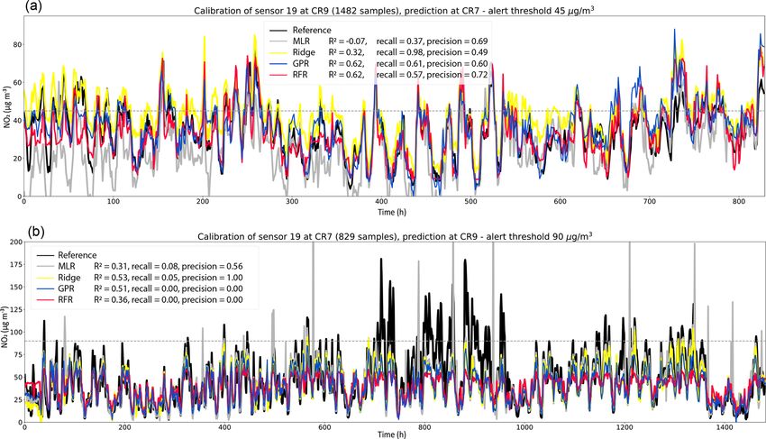
5638                                                                            P. Nowack et al.: Machine learning calibration

et al., 2019; Eilenberg et al., 2020; Sayahi et al., 2020). Here     oratory calibrations do not always perform well in the field
we present insights from a case study using low-cost air pol-        (Castell et al., 2017; Zimmerman et al., 2018). Here, we in-
lution sensors for measurements at three separate locations          stead evaluate the performance of low-cost sensor calibra-
in the urban area of London, UK. Our focus is on testing             tions based on co-location measurements with established
the advantages and disadvantages of machine learning cali-           reference stations (e.g. Masson et al., 2015; Spinelle et al.,
bration techniques for low-cost NO2 and PM10 sensors. The            2015; Esposito et al., 2016; Lewis et al., 2016; Cross et al.,
principal idea is to calibrate the sensors through co-location       2017; Hagan et al., 2018; Casey and Hannigan, 2018; Casey
with established high-performance air pollution measure-             et al., 2019; De Vito et al., 2018, 2019; Zimmerman et al.,
ment stations (Fig. 1). Such calibration techniques, if suc-         2018; Casey et al., 2019; Munir et al., 2019; Malings et al.,
cessful, could complement more expensive laboratory-based            2019, 2020). If sufficiently successful, these methods could
calibration approaches, thereby further reducing the costs of        help to substantially reduce the overall costs and simplify the
the overall measurement process (e.g. Spinelle et al., 2015;         process of calibrating low-cost sensors.
Zimmerman et al., 2018; Munir et al., 2019). For the sen-                Another challenge in relation to co-location calibration
sor calibration, we compare three machine learning regres-           procedures is “site transferability”. This term refers to the
sion techniques in the form of ridge regression, random for-         measurement performance implications of moving a cali-
est regression (RFR) and Gaussian process regression (GPR),          brated device from one location (where the calibration was
and we contrast the results to those obtained with standard          conducted) to another location. Some significant perfor-
multiple linear regression (MLR). RFR has been studied in            mance losses after site transfers have been reported (e.g.
the context of NO2 co-location calibrations before, with very        Fang and Bate, 2017; Casey and Hannigan, 2018; Hagler
promising results (Zimmerman et al., 2018). Equally for NO2          et al., 2018; Vikram et al., 2019), with reasons typically not
(but not for PM10 ) different linear versions of GPR have been       being straightforward to assign. A key driver might be that
tested by De Vito et al. (2018) and Malings et al. (2019).           often devices are calibrated in an environment not repre-
To the best of our knowledge, we are the first to test ridge         sentative of situations found in later measurement locations.
regression both for NO2 and PM10 and GPR for PM10 . Fi-              As we discuss in greater detail below, for machine-learning-
nally, we also investigate well-known issues concerning site         based calibrations this behaviour can, to a degree, be fairly
transferability (Masson et al., 2015; Fang and Bate, 2017;           intuitively explained by the fact that they do not tend to per-
Hagan et al., 2018; Malings et al., 2019), i.e. if a calibra-        form well when extrapolating beyond their training domain.
tion through co-location at one location gives rise to reliable      As we will show, this issue can easily occur in situations
measurements at a different location.                                where already calibrated sensors have to measure pollution
   A key motivation for our study is the potential of low-           levels well beyond the range of values encountered in their
cost sensors (costs of the order of GBP 10 to GBP 100) to            training environment.
transform the level of availability of air pollution measure-            We highlight that, in particular concerning the perfor-
ments. Installation costs of state-of-the-art measurement sta-       mance of low-cost PM10 sensors, a huge gap in the scien-
tions typically range between GBP 10 000 and GBP 100 000             tific literature has been identified regarding issues related to
per site, and those already high costs are further exacer-           co-location calibrations (Rai and Kumar, 2018). We there-
bated through subsequent maintenance and calibration re-             fore expect that our study will provide novel insights into
quirements (Mead et al., 2013; Lewis et al., 2016; Castell           the effects of different calibration techniques on sensor per-
et al., 2017). Lower measurement costs would allow for the           formances, and a data sample that other measurement stud-
deployment of denser air pollution sensor networks and for           ies from academia and industry can compare their results
portable devices possibly even at the exposure level of indi-        against. We will mainly use the R 2 score (coefficient of de-
viduals (Mead et al., 2013). A central complication is the sen-      termination) and root mean squared error (RMSE) as metrics
sitivity of sensors to environmental conditions such as tem-         to evaluate our calibration results, which are widely used and
perature and relative humidity (Masson et al., 2015; Spinelle        should thus facilitate intercomparisons. To provide a refer-
et al., 2015; Jiao et al., 2016; Lewis et al., 2016; Spinelle        ence for calibration results perceived as “good” for PM10 ,
et al., 2017; Castell et al., 2017) or to cross-sensitivities with   we point towards a sensor comparison by Rai and Kumar
other gases (e.g. nitrogen oxide), which can significantly im-       (2018), who found that low-cost sensors generally displayed
pede their measurement performance (Mead et al., 2013;               moderate to excellent linearity (R 2 > 0.5) across various cal-
Popoola et al., 2016; Rai and Kumar, 2018; Lewis et al.,             ibration settings. The sensors typically perform particularly
2018; Liu et al., 2019). Low-cost sensors thus require, in           well (R 2 > 0.8) when tested in idealized laboratory condi-
the same way as many other measurement devices, sophis-              tions. However, their performance is generally lower in field
ticated calibration techniques. Machine learning regressions         deployments (see also Lewis et al., 2018). For PM10 , this per-
have seen increased use in this context due to their ability         formance deterioration was, inter alia, attributed to changing
to calibrate for many simultaneous, non-linear dependencies.         conditions of particle composition, particle sizes and envi-
These dependencies, in turn, can for example be assessed in          ronmental factors such as humidity and temperature, which
relatively expensive laboratory settings. However, even lab-         are thus important factors to account for in our calibrations.

Atmos. Meas. Tech., 14, 5637–5655, 2021                                               https://doi.org/10.5194/amt-14-5637-2021

P. Nowack et al.: Machine learning calibration 5639
Figure 1. Sketch of the co-location calibration methodology. We co-locate several low-cost sensors for PM (for various particle sizes)
and NO2 with higher-cost reference measurement stations for PM10 and NO2 . The low-cost sensors also measure relative humidity and
temperature as key environmental variables that can interfere with the sensor signals, and for NO2 calibrations, we further include nitrogen
oxide (NO) sensors. We formulate the calibration task as a regression problem in which the low-cost sensor signals and the environmental
variables are the predictors (Xr ) and the reference station signal the predictand (Yr ), both measured at the same location r. The time resolution
is set to hourly averages to match publicly available reference data. We train separate calibration functions for each NO2 and PM10 sensor,
and we compare three different machine learning algorithms (ridge, random forest and Gaussian process regressions) with multiple linear
regression in terms of their respective calibration performances. The performance is evaluated on out-of-sample test data, i.e. on data not
used during training. Once trained and cross-validated, we use these calibration functions to predict PM10 and NO2 concentrations given
new low-cost measurements X, either measured at the same location r or at a new location r 0 . The latter location is to test the feasibility and
impacts of changing measurement sites post-calibration. The time series (right) are for illustration purposes only.
The structure of our paper is as follows. In Sect. 2, we PM2.5 , ozone). A caveat is that appropriate co-location data
introduce the low-cost sensor hardware used, the reference from higher-cost reference measurements might not always
measurement sources, the three measurement site character- be available.
istics and measurement periods, the four calibration regres- For NO2 , we incorporated three different types of sensors
sion methods, and the calibration settings (e.g. measured sig- in our set-up for which purchasing prices differed by an or-
nals used) for NO2 and PM10 . In Sect. 3, we first introduce der of magnitude. One aspect of our study will therefore be
multi-sensor calibration results for NO2 at a single site, de- to evaluate the performance gained by using the more expen-
pending on the sensor signals included in the calibrations and sive (but still relatively low-cost) sensor types. Of course, our
the number of training samples used to train the regressions. results will only be validated in the context of our specific
This is followed by a discussion of single-site PM10 calibra- calibration method so that more general conclusions have to
tion results before we test the feasibility and challenges of be drawn with care.
site transfers. We discuss our results and draw conclusions in Each multi-sensor node contained the following (i.e. all
Sect. 4. nodes consist of the same types of individual sensors):
– Two MiCS-2714 NO2 sensors produced by SGX Sen-
2 Methods and data sortech. These are the cheapest measurement devices
deployed in our set with market costs of approximately
2.1 Sensor hardware GBP 5 per sensor.
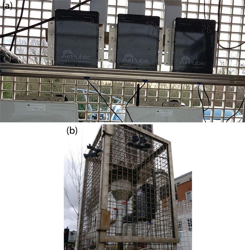
Depending on the measurement location, we deployed one – Two Plantower PMS5003T series PM sensors (PMSs),
set or several sets of air pollution sensors, and we refer to which measure particles of various size categories in-
each set (provided by London-based AirPublic Ltd) as a cluding PM10 based on laser scattering using Mie the-
multi-sensor “node”. Each of these nodes consists of multiple ory. We note that particle composition does play a role
electrochemical and metal oxide sensors for PM and NO2 , as in any PM calibration process as, for example, organic
well as sensors for environmental quantities and other chemi- materials tend to absorb a higher proportion of inci-
cal species known for potential interference with their sensor dent light as compared to inorganic materials (Rai and
signals (required for calibration). Each node thus allows for Kumar, 2018). Below we therefore effectively make
simultaneous measurement of multiple air pollutants, but we the assumption that we measure and calibrate within
will focus on individual calibrations for NO2 and PM10 here, composition-wise similar environments. By taking into
because these species were of particular interest to our own account various particle size measures in the calibra-
measurement campaigns. We note that other species such as tion, we likely do indirectly account for some aspects of
PM2.5 are also included in the measured set of variables. We composition though, because to a degree, particle sizes
will make our low-cost sensor data available (see “Data avail- might be correlated with particle composition. Each
ability” section), which will allow other users to test simi- PMS device also contains a temperature and relative hu-
lar calibration procedures for other variables of interest (e.g. midity sensor, and these variables were also included in
https://doi.org/10.5194/amt-14-5637-2021 Atmos. Meas. Tech., 14, 5637–5655, 2021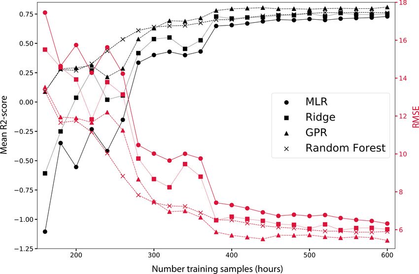
5640                                                                          P. Nowack et al.: Machine learning calibration

      our calibrations. The minimum distinguishable particle     2.3     Co-location set-up and calibration variables
      diameter for the PMS devices is 0.3 µm. The market cost
      is GBP 20 for one sensor.                                  In total, we co-located up to 30 nodes, labelled by identi-
                                                                 fiers (IDs) 1 to 30. For our NO2 measurements, we consid-
  – An NO2-A43F four-electrode NO2 sensor produced by
                                                                 ered the following 15 sensor signals per node to be important
    AlphaSense (market cost GBP 45).
                                                                 for the calibration process: the NO sensor (plus its baseline
  – An NO2-B43F four-electrode NO2 sensor produced by            signal to remove noise), the NO2 + O3 sensor (plus base-
    AlphaSense (market cost GBP 45).                             line), the two intermediate cost NO2 sensors (NO2-A43F,
                                                                 NO2-B43F) plus their respective baselines, the two cheaper
  – An NO-A4 four-electrode nitric oxide sensor produced         MiCS sensors, three different temperature sensors, and two
    by AlphaSense to calibrate against the sometimes sig-        relative humidity sensors. All 15 signals can be used for cali-
    nificant interference of NO2 signals with NO (market         bration against the reference measurements obtained with the
    cost GBP 45).                                                co-located higher-cost measurement devices. We discuss the
                                                                 relative importance of the different signals, e.g. the relative
  – An OX-A431 four-electrode oxidizing gas sensor mea-          importance of the different NO2 sensors or the influence of
    suring a combined signal from ozone and NO2 produced         temperature and humidity in Sect. 3. For the PM10 calibra-
    by AlphaSense. We used this signal to calibrate against      tions, we used two devices of the same type of low-cost PM
    possible interference of electrochemical NO2 measure-        sensor, resulting in 2×10 different particle measures used in
    ments by ozone (market cost GBP 45).                         the PM10 calibrations. In addition, we included the respective
                                                                 sensor signals for temperature and relative humidity, provid-
  – A separate temperature sensor built into the AlphaSense
                                                                 ing us with in total 24 calibration signals for PM10 .
    set. It is needed to monitor the warm-up phase of the
    sensors.
                                                                 2.4     Calibration algorithms
In normal operation mode, each node provided measure-
ments around every 30 s. These signals were time-averaged        We evaluate four regression calibration strategies for low-
to hourly values for calibration against hourly public refer-    cost NO2 and PM10 devices, by means of co-location of
ence measurements.                                               the devices with the aforementioned air quality measurement
                                                                 reference stations. The four different regression methods –
2.2    Measurement sites and reference monitors
                                                                 which are multiple linear regression (MLR), ridge regres-
We conducted measurements at three sites in the Greater          sion, random forest regression (RFR) and Gaussian process
London area during distinct multi-week periods (Table 1).        regression (GPR) – are introduced in detail in the following
Two of the sites are located in the London Borough of Croy-      subsections. As we will show in Sect. 3, the relative skill of
don, which we label CR7 and CR9 according to their UK            the calibration methods depends on the chemical species to
postcodes. The third site is located in the car park of the      be measured, sample size available for calibration, and cer-
company AlphaSense in Essex, hereafter referred to as site       tain user preferences. We will additionally consider the issue
“CarPark” (Fig. 2a). At CR7, the sensor nodes were located       of site transferability for sensor node 19, including its depen-
kerbside on a medium busy street with two lanes in either        dence on the calibration algorithm used. We note that we do
direction. At CR9, the nodes were located on a traffic island    not include the manufacturer calibration of the low-cost sen-
                                                                 sors in our comparison here mainly because we found that
in the middle of a very busy road with three lanes in either
direction (Fig. 2b). For the two Croydon sites, reference mea-   this method, which is a simple linear regression based on cer-
surements were obtained from co-located, publicly available      tain laboratory measurement relationships, provided us with
measurements of London’s Air Quality Network (LAQN;              negative R 2 scores when compared with reference sensors in
https://www.londonair.org.uk, last access: 30 April 2020). In    the field. This result is in line with other studies that reported
the two locations in question, the LAQN used chemilumi-          differences between sensor performances in the field and un-
nescence detectors for NO2 and Thermo Scientific tapered         der laboratory calibrations (see e.g. Mead et al., 2013; Lewis
element oscillating microbalance (TEOM) continuous ambi-         et al., 2018; Rai and Kumar, 2018).
ent particulate monitors, with the Volatile Correction Model
(Green et al., 2009) for PM10 measurements at CR9. For           2.4.1    Ridge and multiple linear regression
the CarPark site, PM10 measurements were conducted with
a Palas Fidas optical particle counter AFL-W07A. These           Ridge regression is a linear least squares regression aug-
CarPark reference measurements were provided at 15 min in-       mented by L2 regularization to address the bias-variance
tervals. For consistency, these measurements were averaged       trade-off (Hoerl and Kennard, 1970; James et al., 2013;
to hourly values to match the measurement frequency of pub-      Nowack et al., 2018, 2019). Using statistical cross-validation,
licly available data at the other two sites.                     the regression fit is optimized by minimizing the cost func-

Atmos. Meas. Tech., 14, 5637–5655, 2021                                            https://doi.org/10.5194/amt-14-5637-2021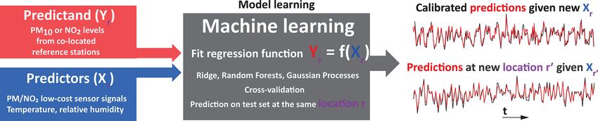
P. Nowack et al.: Machine learning calibration                                                                                              5641

Table 1. Overview of the measurement sites and the corresponding maximum co-location periods, which vary for each specific sensor
node and co-location site due to practical aspects such as sensor availability and random occurrences of sensor failures. Note that reference
measurements for NO2 and PM10 are only available for two of the three sites each. Sensors that were co-located for at least 820 active
measurement hours are identified by their sensor IDs in the last column. Further note that the only sensor used to measure at multiple sites is
sensor 19, which is therefore used to test the feasibility of site transfers.

   Site          Max co-location period                          Reference sensors                                       Low-cost sensor IDs
   CR7           22 October–5 December 2018                      NO2 (London Air Quality Network)                        3–7, 11, 13–24, 27, 28
   CR9           24 September 2019–19 January 2020               NO2 and PM10 (London Air Quality Network)               19
   CarPark       29 January–26 April 2019                        PM10 (Palas Fidas optical particle counter AFL-W07A)    19, 25, 26

Figure 2. Examples of the co-location set-up of the AirPublic low-cost sensor nodes with reference measurement stations at sites (a) CarPark
and (b) CR9.

tion                                                                             signals from the low-cost sensors, representing signals for
                                          !2                                     the pollutant itself as well as signals recorded for environ-
           n             p                          p
           X             X                          X                            mental variables (temperature, humidity) and other chemical
JRidge =          yt −          cj xj,t        +α          cj2           (1)     species that might cause interference with the signal in ques-
           t=1           j =1                       j =1
                                                                                 tion. The cost function (Eq. 1) determines the optimization
over n hourly reference measurements of pollutant y (i.e.                        goal. Its first term is the ordinary least squares regression er-
NO2 , PM10 ); xj,t represents p non-calibrated measurement                       ror, and the second term puts a penalty on too large regression

https://doi.org/10.5194/amt-14-5637-2021                                                           Atmos. Meas. Tech., 14, 5637–5655, 2021
5642                                                                           P. Nowack et al.: Machine learning calibration

coefficients and thus avoids overfitting in high-dimensional        units). As a result, the predictors would be penalized differ-
settings. Smaller (larger) values of the regularization coeffi-     ently through the same α in Eq. (1), which could mean that
cient α put weaker (stronger) constraints on the size of the co-    certain predictors are effectively not considered in the regres-
efficients, thereby favouring overfitting (high bias). We find      sions. Here, we normalize all predictors in all regressions to
the value for α through fivefold cross-validation; i.e. each        zero mean and unit standard deviation according to the sam-
data set is split into five ordered time slices and α optimized     ples included in each training data set.
by fitting regressions for large ranges of α values on four of
the slices at a time, and then the best α is found by evaluating    2.4.2   Random forest regression
the out-of-sample prediction error on each corresponding re-
maining slice using the R 2 score. Each slice is used once for      Random forest regression (RFR) is one of the most widely
the evaluation step. Before the training procedure, all signals     used non-linear machine learning algorithms (Breiman and
are scaled to unit variance and zero mean so as to ensure that      Friedman, 1997; Breiman, 2001), and it has already found
all signals are weighted equally in the regression optimiza-        applications in air pollution sensor calibration as well as in
tion, which we explain in more detail at the end of this sec-       other aspects of atmospheric chemistry (Keller and Evans,
tion. Through the constraint on the regression slopes, ridge        2019; Nowack et al., 2018, 2019; Sherwen et al., 2019; Zim-
regression can handle settings with many predictors, here           merman et al., 2018; Malings et al., 2019). It follows the idea
calibration variables, even in the context of strong collinear-     of ensemble learning where multiple machine learning mod-
ity in those predictors (Dormann et al., 2013; Nowack et al.,       els together make more reliable predictions than the individ-
2018, 2019). The resulting linear regression function fRidge ,      ual models. Each RFR object consists of a collection (i.e. en-
                        p
                                                                    semble) of graphical tree models, which split training data by
                        X                                           learning decision rules (Fig. 3). Each of these decision trees
ŷ(t) = fRidge = c0 +          cj xj (t),                    (2)
                        j =1
                                                                    consists of a sequence of nodes, which branch into multi-
                                                                    ple tree levels until the end of the tree (the “leaf” level) is
provides estimates for pollutant mixing ratios ŷ at any time       reached. Each leaf node contains at least one or several sam-
t, i.e. a calibrated low-cost sensor signal, based on new sen-      ples from the training data. The average of these samples is
sor readings xj (t). fRidge represents a calibration function       the prediction of each tree for any measurement of predic-
because it is not just based on a regression of the pollutant       tors x defining a new traversion of the tree to the given leaf
signal itself against the reference but also on multiple simul-     node. In contrast to ridge regression, there is more than one
taneous predictors, including those representing known inter-       tunable hyperparameter to address overfitting. One of these
fering factors.                                                     hyperparameters is the maximum tree depth, i.e. the maximal
   Multiple linear regression (MLR) is the simple non-              number of levels within each tree, as deeper trees allow for
regularized case of ridge regression, i.e. where α is set to nil.   a more detailed grouping of samples. Similarly, one can set
MLR is therefore a good benchmark to evaluate the impor-            the minimum number of samples in any leaf node. Once this
tance of regularization and, when compared to RFR and GPR           minimum number is reached, the node is not further split into
below, of non-linearity in the relationships. As MLR does           children nodes. Both smaller tree depth and a greater number
not regularize its coefficients, it is expected to increasingly     of minimum samples in leaf nodes mitigate overfitting to the
lose performance in settings with many (non-linear) calibra-        training data. Other important settings are the optimization
tion relationships. This loss of MLR performance in high-           function used to define the decision rules and, for example,
dimensional regression spaces is related to the “curse of di-       the number of estimators included in an ensemble, i.e. the
mensionality” in machine learning, which expresses the ob-          number of trees in the forest.
servation that one requires an exponentially increasing num-           The RFR training process tunes the parameter thresholds
ber of samples to constrain the regression coefficients as the      for each binary decision tree node. By introducing random-
number of predictors is increased linearly (Bishop, 2006).          ness, e.g. by selecting a subset of samples from the train-
We will illustrate this phenomenon for the case of our NO2          ing data set (bootstrapping), each tree provides a somewhat
sensor calibrations below.                                          different data representation. This random element is used
   Finally, we note that for ridge regression, as also for GPR      to obtain a better, averaged prediction over all trees in the
described below, the predictors xj must be normalized to            ensemble, which is less prone to overfitting than individual
a common range. For ridge, this is straightforward to un-           regression trees. We here cross-validated the scikit-learn im-
derstand as the regression coefficients, once the predictors        plementation of RFR (Pedregosa et al., 2011) over problem-
are normalized, provide direct measures of the importance           specific ranges for the minimum number of samples required
of each predictor for the overall pollutant signal. If not nor-     to define a split and the minimum number of samples to de-
malized, the coefficients will additionally weight the relative     fine a leaf node. The implementation uses an optimized ver-
magnitude of predictor signals, which can differ by orders          sion of the Classification And Regression Tree (CART) algo-
of magnitude (e.g. temperature at around 273 K but a mea-           rithm, which constructs binary decision trees using the pre-
surement signal for a trace gas of the order of 0.5 amplifier       dictor and threshold that yields the largest information gain

Atmos. Meas. Tech., 14, 5637–5655, 2021                                              https://doi.org/10.5194/amt-14-5637-2021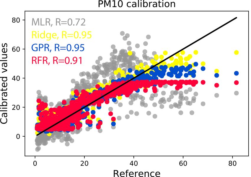
P. Nowack et al.: Machine learning calibration                                                                                            5643

Figure 3. Sketch of a random forest regressor. Each random forest consists of an ensemble of K trees. For visualization purposes, the trees
shown here have only four levels of equal depth, but more complex structures can be learnt. The lowest level contains the leaf nodes. Note that
in real examples, branches can have different depths; i.e. the leaf nodes can occur at different levels of the tree hierarchy; see, for example,
Fig. 2 in Zimmerman et al. (2018). Once the decision rules for each node and tree are learnt from training data, each tree can be presented
with new sensor readings x at a time t to predict pollutant concentration yt . The decision rules depend, inter alia, on the tree structure and
random sampling through bootstrapping, which we optimize through fivefold cross-validation. Based on the values xi , each set of predictors
follows routes through the trees. The training samples collected in the corresponding leaf node define the tree-specific prediction for y. By
averaging K tree-wise predictions, we combat tree-specific overfitting and finally obtain a more regularized random forest prediction y t .

for a split at each node. The mean squared error of samples               air pollution sensor signals, we here use a sum kernel of a
relative to their node prediction (mean) serves as optimiza-              radial basis function (RBF) kernel, a white noise kernel, a
tion criterion so as to measure the quality of a split for a given        Matérn kernel and a “Dot-Product” kernel. The RBF kernel,
possible threshold during training. Here we consider all fea-             also known as squared exponential kernel, is defined as
tures when defining any new best split of the data at nodes.                                              !
By increasing the number of trees in the ensemble, the RFR                                  −d(xi , xj )2
                                                                          k(xi , xj ) = exp                 .                     (4)
generalization error converges towards a lower limit. We here                                    2l 2
set the number of trees in all regression tasks to 200 as a
compromise between model convergence and computational                    It is parameterized by a length scale l > 0, and d is the Eu-
complexity (Breiman, 2001).                                               clidean distance. The length scale determines the scale of
                                                                          variation in the data, and it is learnt during the Bayesian
2.4.3   Gaussian process regression                                       update; i.e. for a shorter length scale the function is more
                                                                          flexible. However, it also determines the extrapolation scale
Gaussian process regression (GPR) is a widely used                        of the function, meaning that any extrapolation beyond the
Bayesian machine learning method to estimate non-linear                   length scale is probably unreliable. RBF kernels are partic-
dependencies (Rasmussen and Williams, 2006; Pedregosa                     ularly helpful to model smooth variations in the data. The
et al., 2011; Lewis et al., 2016; De Vito et al., 2018; Runge             Matérn kernel is defined by
et al., 2019; Malings et al., 2019; Nowack et al., 2020; Mans-
                                                                                                    √                !ν
field et al., 2020). In GPR, the aim is to find a distribution                             1          2ν
over possible functions that fit the data. We first define a prior        k(xi , xj ) =                   d(xi , xj ) Kν
                                                                                        0(ν)2ν−1      l
distribution of possible functions that is updated according                             √               !
to the data using Bayes’ theorem, which provides us with a                                 2ν
posterior distribution over possible functions. The prior dis-                                d(xi , xj ) ,                         (5)
                                                                                           l
tribution is a Gaussian process (GP),
                                                                         where Kν is a modified Bessel function and 0 the gamma
Y ∼ GP µ, k(xi , xj ) ,                                        (3)        function (Pedregosa et al., 2011). We here choose ν = 1.5
                                                                          as the default setting for the kernel, which determines the
with mean µ and a covariance function or kernel k, which                  smoothness of the function. Overall, the Matérn kernel is
describes the covariance between any two points xi and xj .               useful to model less-smooth variations in the data than the
We here “standard-scale” (i.e. centre) our data so that µ = 0,            RBF kernel. The Dot-Product kernel is parameterized by a
meaning our GP is entirely defined by the covariance func-                hyperparameter σ02 ,
tion. Being a kernel method, the performance of GPR de-
pends strongly on the kernel (covariance function) design as              k(xi , xj ) = σ02 + xi · xj ,                                     (6)
it determines the shape of the prior and posterior distributions
of the Gaussian process and in particular the characteristics             and we found that adding this kernel to the sum of kernels
of the function we are able to learn from the data. Owing                 improved our results empirically. The white noise kernel sim-
to the time-varying, continuous but also oscillating nature of            ply allows for a noise level on the data as independently

https://doi.org/10.5194/amt-14-5637-2021                                                      Atmos. Meas. Tech., 14, 5637–5655, 2021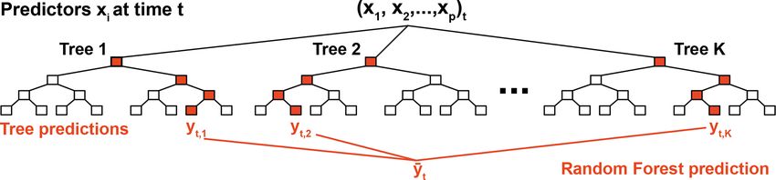
5644                                                                             P. Nowack et al.: Machine learning calibration

and identically normally distributed, specified through a vari-      ranges encountered for the predictors (e.g. low-cost sensor
ance parameter. This parameter is similar to (and will interact      signals, humidity, temperature) and predictands (reference
with) the α noise level described below, which is, however,          NO2 , PM10 ). The calibration range in turn affects the per-
tested systematically through cross-validation.                      formance of the calibration function: if faced with values out-
   The Python scikit-learn implementation of the algorithm           side its training range, the function effectively has to perform
used here is based on Algorithm 2.1 of Rasmussen and                 an extrapolation rather than interpolation, i.e. the function is
Williams (2006). We optimized the kernel parameters in the           not well constrained outside its training domain. This lim-
same way as for the other regression methods through five-           itation is particularly critical for non-linear machine learn-
fold cross-validation, and we subject them to the noise α pa-        ing functions (Hagan et al., 2018; Nowack et al., 2018; Zim-
rameter of the scikit-learn GPR regression packages (Pe-             merman et al., 2018). Calibration performance will further
dregosa et al., 2011). This parameter is not to be confused          vary for each device, even for sensors of the same make, due
with the α regularization parameter for ridge regression and         to unavoidable randomness in the sensor production process
takes the role of smoothing the kernel function so as to ad-         (Mead et al., 2013; Castell et al., 2017). To characterize these
dress overfitting. It represents a value added to the diagonal       various influences, we here test the dependence of three ma-
of the kernel matrix during the fitting process with larger α        chine learning calibration methods, as well as of MLR, on
values corresponding to greater noise level in the measure-          sample size and co-location period for a number of NO2 sen-
ments of the outputs. However, we note that there is some            sors.
equivalency with the α parameter in ridge as the method                 The NO2 co-location data at CR7 is ideally suited for this
is effectively a form of Tikhonov regularization that is also        purpose. Twenty-one sensor nodes of the same make were
used in ridge regression (Pedregosa et al., 2011). Both inputs       co-located with a LAQN reference during the period Octo-
and outputs to the GPR function were standard-scaled to zero         ber to December 2018 (Table 1). We actually co-located 30
mean and unit variance based on the training data. For each          sensor sets at the site, but we excluded any sensors with less
GPR optimization, we chose 25 optimizer restarts with dif-           than 820 h (samples) after outlier removal from our evalua-
ferent initializations of the kernel parameters, which is nec-       tion. The remaining sensors measure sometimes overlapping
essary to approximate the best possible solution to maximize         but still distinct time periods, because each sensor measure-
the log-marginal likelihood of the fit. More background on           ment varied in its precise co-location start and end time and
GPR can be found in Rasmussen and Williams (2006).                   was also subject to sensor-specific periods of malfunction. To
                                                                     detect these malfunctions, and to exclude the corresponding
2.5    Cross-validation                                              samples, we removed outliers (evidenced by unrealistically
                                                                     large measurement signals) at the original time resolution of
For all regression models, we performed fivefold cross-              our measurements, i.e. < 1 min and prior to hourly averag-
validation where the data are first split into training and test     ing. To detect outliers for removal, we used the median ab-
sets, keeping samples ordered by time. The training data are         solute deviation (MAD) method, also known as “robust Z-
afterwards divided into five consecutive subsets (folds) of          Score method”, which identifies outliers for each variable
equal length. If the training data are not divisible by five, with   based on their univariate deviation from their training data
a residual number of samples n, then the first n folds will          median. Since the median is a robust statistic to outliers it-
contain one surplus sample compared to the remaining folds.          self, it is a typically a better measure to identify outliers than,
Each fold is used once as a validation set, while the remain-        for example, a deviation from the mean. Accordingly, we ex-
ing four folds are used for training. The best set of model hy-      cluded any samples t from the training and test data where
perparameters or kernel functions is found according to the          the quantity
average generalization error on these validation sets. After
the best cross-validated hyperparameters are found, we refit                             |xj,t − x̃j |
the regression models on the entire training data using these        Mj,t = 0.6745                                                 (7)
                                                                                     median |xj,t − x̃j |
hyperparameter settings (e.g. the α value for which we found
the best out-of-sample performance for ridge regression).            takes on values > 7 for any of the predictors, where x̃j is
                                                                     the training data median value of each predictor. To train and
3     Results                                                        cross-validate our calibration models, we took the first 820 h
                                                                     measured by each sensor set and split it into 600 h for train-
3.1    NO2 sensor calibration                                        ing and cross-validation, leaving 220 h to measure the final
                                                                     skill on an out-of-sample test set. We highlight again that the
The skill of a sensor calibration function is expected to in-        test set will cover different time intervals for different sen-
crease with sample size, i.e. the number of measurements             sors, meaning that further randomness is introduced in how
used in the calibration process, but will also depend on as-         we measure calibration skill. However, the relationships for
pects of the sampling environment. For co-location measure-          each of the four calibration methods are learnt from exactly
ments, there will be time-dependent fluctuations in the value        the same data and their predictions are also evaluated on the

Atmos. Meas. Tech., 14, 5637–5655, 2021                                                https://doi.org/10.5194/amt-14-5637-2021
P. Nowack et al.: Machine learning calibration 5645
same data, meaning that their robustness and performance 3.1.1 Comparison of regression models for all
can still be directly compared. To measure calibration skill, predictors
we used two standard metrics in the form of the R 2 score
(coefficient of determination), defined by For a first comparison of the calibration performance of the
Pn four methods, we show R 2 scores and RMSEs in Table 2,
(yi − ŷi )2 rows (a) to (c), averaged across all 21 sensor nodes. GPR
R (y, ŷ) = 1 − Pi=1
2
n 2
, (8) emerges as the best-performing method for all three sets of
i=1 (yi − y)
predictor choices, reaching R 2 scores better than 0.8 for I30
and the RMSE between the reference measurements y and and I45 . This highlights that GPR should from now on be
our calibrated signals ŷ on the test sets. For particularly poor considered an option in similar sensor calibration exercises.
calibration functions, the R 2 score can take on infinitely neg- RFR consistently performs worse than GPR but slightly bet-
ative values, whereas a value of 1 implies a perfect predic- ter than ridge regression, which in turn outperforms MLR
tion. An R 2 score of 0 is equivalent to a function that pre- in all cases, but the differences are fairly small for I15 and
dicts the correct long-term time average of the data but no I30 . A notable exception occurs for I45 , where the R 2 score
fluctuations therein. for MLR suddenly drops abruptly to around 0.2. This sudden
As discussed in Sect. 2.1, each of AirPublic’s co-location performance loss can be understood from the aforementioned
nodes measures 15 signals (the predictors or inputs) that we curse of dimensionality: MLR increasingly overfits the train-
consider relevant for the NO2 sensor calibration against the ing data as the number of predictors increases; the existing
LAQN reference signal for NO2 (the predictand or output). sample size becomes too small to constrain the 45 regres-
Each of the 15 inputs will potentially be systematically lin- sion coefficients (Bishop, 2006; Runge et al., 2012). The ma-
early or non-linearly correlated with the output, which al- chine learning methods can deal with this increase in dimen-
lows us to learn a calibration function from the measure- sionality highly effectively and thus perform well through-
ment data. Once we know this function, we should be able out all three cases. Indeed, GPR and ridge regression benefit
to make accurate predictions given new inputs to reproduce slightly from the additional predictor transformations. This
the LAQN reference. As we fit two linear and two non-linear robustness to regression dimensionality is a first central ad-
algorithms, certain transformations of the inputs can be use- vantage of machine learning methods in sensor calibrations.
ful to facilitate the learning process. For example, a relation- Machine learning methods will be more reliable and will al-
ship between an input and the output might be an exponen- low users to work in a higher-dimensional calibration space
tial dependence in the original time series so that applying compared to MLR. Having said that, for 15 input features
a logarithmic transformation could lead to an approximately the performance of all methods appears very similar on first
linear relationship that might be easier to learn for a linear re- sight, making MLR seemingly a viable alternative to the ma-
gression function. We therefore compared three set-ups with chine learning methods. We note, however, that there is no
different sets of predictors: apparent disadvantage in using machine learning methods to
prevent potential dangers of overfitting depending on sample
1. using the 15 input time series as provided (label I15 );
size.
2. adding logarithmic transformations of the predictors
(I30 ); and 3.1.2 Calibration performance depending on sample
size
3. adding both logarithmic and exponential transforma-
tions of the predictors (I45 ). We next consider the performance dependence on sample
size of the training data (Fig. 4). The advantages of machine
These are labelled according to their total number of predic- learning methods become even more evident for smaller
tors after adding the input transformations, i.e. 15, 30 and numbers of training samples, even if we consider case (b)
45. The logarithmic and exponential transformations of each with 30 predictors, i.e. I30 , for which we found that MLR
input signal Ai (t) are defined as performs fairly well if trained on 600 h of data. The mean
R 2 score and RMSE (µg m−3 ) quickly deteriorate for smaller
Ai,log (t) = log (Ai (t) + 1) , (9a) sample sizes for MLR, in particular below a threshold of less
Ai (t) than 400 h of training data. Ridge regression – its statistical
Ai,exp (t) = exp , (9b) learning equivalent – always outperforms MLR. Both GPR
Amax +
and RFR can already perform well at small samples sizes of
where Amax is the maximum value of the predictor time se- less than 300 h. While all methods converge towards similar
ries, and = 10−9 . The latter prevents possible divisions by performance approaching 600 h of training data (Table 2),
zero, whereas the former prevents overflow values in the MLR is generally performing worse than ridge regression
function. and significantly worse that RFR and GPR.
https://doi.org/10.5194/amt-14-5637-2021 Atmos. Meas. Tech., 14, 5637–5655, 20215646 P. Nowack et al.: Machine learning calibration
Table 2. Average NO2 sensor skill depending on the selection of predictors. Shown are average R 2 scores and root mean squared errors (in
brackets; units µg m−3 ). Results are averaged over the 21 low-cost sensor nodes with 600 hourly training samples each, and the evaluation is
carried out for 220 test samples each. RH stands for relative humidity, and T stands for temperature.
Input features MLR Ridge RFR GPR
(a) I15 0.74 (6.2) 0.75 (6.1) 0.76 (5.9) 0.79 (5.7)
(b) I30 0.73 (6.3) 0.75 (6.0) 0.76 (5.9) 0.81 (5.4)
(c) I45 0.23 (10.6) 0.75 (6.0) 0.76 (5.9) 0.80 (5.5)
(d) MiCS, T , RH −2.9 (28.3) −0.03 (12.6) 0.01 (12.2) −0.12 (13.1)
(e) A43F, T , RH 0.25 (9.7) 0.22 (10.1) 0.44 (8.7) 0.47 (8.4)
(f) B43F, T , RH 0.20 (10.6) 0.39 (9.7) 0.43 (9.5) 0.49 (9.3)
(g) NO/O3 /B43F/T /RH 0.68 (6.9) 0.75 (6.2) 0.69 (6.8) 0.77 (6.0)
(h) (g) + A43F 0.72 (6.4) 0.74 (6.2) 0.75 (6.1) 0.79 (5.7)
(i) I30 + B43F (τ = 1) 0.78 (5.8) 0.79 (5.6) 0.78 (5.7) 0.84 (5.0)
Further evidence for advantages of machine learning
methods are provided in Fig. 5, showing boxplots of the
R 2 score distributions across all 21 sensor nodes depending
on sample size (300, 400, 500, 600 h) and regression method.
While median sensor performances of MLR, ridge and GPR
ultimately become comparable, MLR is typically found to
yield a number of poor-performing calibration functions with
some R 2 scores well below 0.6 even for 600 training hours.
In contrast, the distributions are far narrower for the machine
learning methods: GPR and RFR do not show a single ex-
treme outlier even after being trained on only 400 h of data,
providing strong indications that the two methods are the
most reliable. After 600 h, one can effectively expect that all
sensors will provide R 2 scores > 0.7 if trained using GPR.
Overall, this highlights again that machine learning methods Figure 4. Error metrics as a function of the number of training sam-
will provide better average skill but are also expected to pro- ples for I30 , as labelled. The figure highlights the convergence of
vide more reliable calibration functions through co-location both metrics for the different regression methods as the sample size
measurements independent of sensor device and the peculiar- increases. Note that MLR would not converge for I45 , owing to the
ities of the individual training and test data set. curse of dimensionality. This tendency can also be seen here for
small sample sizes, where MLR rapidly loses performance. Results
3.1.3 Calibration performance depending on predictor are averaged over the 21 low-cost sensor nodes with 600 hourly
training samples each, and the evaluation is carried out for 220 test
choices and NO2 device
samples each.
Tests (a) to (c) listed in Table 2 indicate that the machine
learning regressions for NO2 , specifically GPR, can bene-
fit slightly from additional logarithmic predictor transforma- We first tested three set-ups in which we used only the
tions but that adding exponential transformations on top of sensor signals of the two cheaper MiCS devices (d) and then
these predictors does not further increase predictive skill, as set-ups with the more expensive AlphaSense A43F (e) and
measured through the R 2 score and RMSE. Incorporating the B43F (f) devices. Using just the MiCS devices, the R 2 score
logarithmic transformations, we next tested the importance drops from 0.75–0.81 for the machine learning methods to
of various predictors to achieve a certain level of calibration around zero, meaning that hardly any of the variation in the
skill (rows (d) to (i) in Table 2). This provides two important true NO2 reference signal is captured. Using our calibration
insights: firstly, we test the predictive skill if we use the in- approach here, the MiCS would therefore not be sufficient
dividual MiCS and AlphaSense NO2 sensors separately, i.e. to achieve a meaningful measurement performance. The pic-
if individual sensors are performing better than others in our ture looks slightly better, albeit still far from perfect, for the
calibration setting and if we need all sensors to obtain the individual A43F and B43F devices for which R 2 scores of
best level of calibration performance. Secondly, we test if almost 0.5 are reached using non-linear calibration meth-
other environmental influences such as humidity and temper- ods. We note that the linear MLR and ridge methods do not
ature significantly affect sensor performance. achieve the same performance, but ridge outperforms MLR.
Atmos. Meas. Tech., 14, 5637–5655, 2021 https://doi.org/10.5194/amt-14-5637-2021P. Nowack et al.: Machine learning calibration 5647
Finally, we note that, in this stationary sensor setting, further
predictive skill can be gained by considering past measure-
ment values. Here, we included the 1 h lagged signal of the
best B43F sensor (i). This is clearly only possible if there is
a delayed consistency (or autocorrelation) in the data, which
here leads to the best average R 2 generalization score of 0.84
for GPR and related gains in terms of the RMSE. While be-
ing an interesting feature, we will not consider such set-ups
in the following, because we intend sensors to be transferable
among locations, and they should only rely on live signals for
the hour of measurement in question.
In summary, using all sensor signals in combination is a
robust and skilful set-up for our NO2 sensor calibration and
is therefore a prudent choice, at least if one of the machine
learning methods is used to control for the curse of dimen-
sionality. In particular, the B43F sensor is important to con-
sider in the calibration, but further calibration skill is gained
by also considering environmental factors, the presence of in-
terference from ozone and NO, and additional NO2 devices.
3.2 PM10 sensor calibration
In the same way as for NO2 , we tested several calibration
settings for the PM10 sensors. For this purpose, we consider
the measurements for the location CarPark, where we co-
located three sensors (IDs 19, 25 and 26) with a higher-cost
device (Table 1). However, after data cleaning, we have only
509 and 439 samples (hours) for sensors 19 and 25 avail-
able, respectively, which our NO2 analysis above indicates
is too short to obtain robust statistics for training and testing
the sensors. Instead we focus our analysis on sensor 26 for
which there are 1314 h of measurements available. We split
these data into 400 samples for training and cross-validation,
leaving 914 samples for testing the sensor calibration. Below
Figure 5. Node-specific I30 R 2 scores depending on calibration we discuss results for various calibration configurations, us-
method and training sample size, evaluated on consistent 220 h ing the 24 predictors for PM10 (Sect. 2.3) and the same four
test data sets in each case (see main text). The boxes extend from regression methods as for NO2 . The baseline case with just
the lower to the upper quartile; inset lines mark the median. The 24 predictors is named I24 , following the same nomencla-
whiskers extending from the box indicate the range excluding out-
ture as for NO2 . I48 and I72 refer to the cases with additional
liers (fliers). Each circle represents the R 2 score on the test set for an
logarithmic and exponential transformations of the predictors
individual node (21 in total). For MLR, some sensor nodes remain
poorly calibrated even for larger sample sizes. according to Eqs. (9a) and (9b). In addition, we test the ef-
fects of environmental conditions, as expressed through rel-
ative humidity and temperature, by excluding these two vari-
ables from the calibration procedure, while using the I48 set-
The most recently developed AlphaSense sensor used in our up with the additional log-transformed predictors.
study, B43F, is the best-performing stand-alone sensor. If we The results of these tests are summarized in Table 3. For
add the NO/ozone sensor as well as the humidity and tem- the baseline case of 24 non-transformed predictors, RFR
perature signals to the predictors – case (g) – its performance (R 2 = 0.70) is outperformed by ridge regression (R 2 = 0.79)
alone almost reaches the same as for the I30 configuration. and GPR (R 2 = 0.79). This is mainly the result of the fact
This implies that the interference with NO/ozone, tempera- that some of the pollution values measured with sensor 26
ture and humidity might be significant and has to be taken during the test period lie outside the range of values encoun-
into account in the calibration, and if only one sensor could tered at training stage. RFR cannot predict values beyond its
be chosen for the measurements, the B43F sensor would be training range (i.e. it cannot extrapolate to higher values) and
the best choice. By further adding the A43F sensor to the can therefore not predict those values accurately (see also
predictors the predictive skill is only mildly improved (h). Zimmerman et al., 2018; Malings et al., 2019). Instead, RFR
https://doi.org/10.5194/amt-14-5637-2021 Atmos. Meas. Tech., 14, 5637–5655, 20215648 P. Nowack et al.: Machine learning calibration
log-transformations have helped linearize certain predictor–
predictand relationships. Further exponential transforma-
tions (I72 ) and thus also further increasing the predictor di-
mensionality did not lead to an improvement in calibration
skill. We therefore ran one final test using the I48 set-up but
without relative humidity and temperature included as pre-
dictors. This test confirmed that the sensor signals indeed ex-
perience a slight interference from humidity and temperature,
at least considering the machine learning regressions. No-
tably, this loss of skill is not observed for MLR for which the
R 2 score actually improves. A likely explanation for this be-
haviour is the curse of dimensionality that affects MLR more
significantly than the three machine learning methods, so the
reduction in collinear dimensions (given the sample size con-
straint) is more beneficial than the information gained by in-
Figure 6. Calibrated PM10 values (in µg m−3 ) versus the reference cluding temperature and humidity in the MLR regression.
measurements for 900 h of test data at location CarPark for the I24 In summary, we have found that ridge regression and GPR
predictor set-up. The ideal 1 : 1 perfect prediction line is drawn in are the two most reliable and high-performing calibration
black. Inset values R are the Pearson correlation coefficients. methods for the PM10 sensor. We are able to attain very good
R 2 scores > 0.7 for all four regression methods though. An
important point to highlight is the characteristics of the train-
constantly predicts the maximum value encountered during ing domain, in particular of the pollution levels encountered
training in those cases. during the training data measurements. If the value range is
However, this problem is not entirely exclusive to RFR but not sufficient to cover the range of interest for future mea-
is inherited by all methods, with RFR only being the most surement campaigns, then ridge regression might be the most
prominent case. We illustrate the more general issue, which robust choice to alleviate the underprediction of the most ex-
will occur in any co-location calibration setting, in Fig. 6. In treme pollution values. However, the power of extrapolation
the training data, there are not any pollution values beyond of any method is limited, so we underline the need to care-
ca. 40 µg m−3 , so the RFR predictions simply level off at that fully check every training data set to see if it fulfils such cru-
value. This is a serious constraint in actual field measure- cial criteria; see also similar discussions in other calibration
ments where one would be particularly interested in episodes contexts (Hagan et al., 2018; Zimmerman et al., 2018; Mal-
of highest pollution. We note that this effect is somewhat al- ings et al., 2019).
leviated by using GPR and even more so by ridge regression.
For the latter, this behaviour is intuitive as the linear relation- 3.3 Site transferability
ships learnt by ridge will hold to a good approximation even
under extrapolation to previously unseen values. However, Finally, we aim to address the question of site transferability,
even for ridge regression the predictions eventually deviate i.e. how reliably a sensor calibrated through co-location can
from the 1 : 1 line for the highest pollution levels. This aspect be used to measure air pollution at a different location. One
will be crucial to consider for any co-location calibration ap- of the sensor nodes (ID 19) was used for NO2 measurements
proach, as is also evident from the poor MLR performance, at both locations, CR7 and CR9, and was also used to mea-
despite being another linear method. In addition, MLR some- sure PM10 at CR9 and CarPark, allowing us to address this
times predicts substantially negative values, producing an question for our methodology. Note that these tests also in-
overall R 2 score of below 0.3, whereas the machine learning clude a shift in the time of year (Table 1), which has been hy-
methods appear to avoid the problem of negative predictions pothesized to be one potentially limiting factor in site trans-
almost entirely. In conclusion, we highlight the necessity for ferability. The results of these transferability tests for PM10
co-location studies to ensure that maximum pollution val- (from CR9 to CarPark and vice versa) and NO2 (from CR7 to
ues encountered during training and testing/deployment are CR9 and vice versa) are shown in Figs. 7 and 8, respectively.
as similar as possible. Extrapolations beyond 10–20 µg m−3 For PM10 , we trained the regressions, using the I24 pre-
appear to be unreliable even if ridge regression is used as cal- dictor set-up, on 400 h of data at either location. This emu-
ibration algorithm, which is the best among our four methods lates a situation in which, according to our results above, we
to combat extrapolation issues. limit the co-location period to a minimum number of sam-
A test with additional log-transformations (I48 ) of the pre- ples required to achieve reasonable performances across all
dictors led to test score improvements for the two linear four regression methods. To mitigate issues related to extrap-
methods (Table 3), in particular for MLR (R 2 = 0.7) but olation (Fig. 6), we selected the last 400 h of the time se-
also for ridge regression (R 2 = 0.8). This implies that the ries for location CarPark (Fig. 7a) and hours 600 to 1000
Atmos. Meas. Tech., 14, 5637–5655, 2021 https://doi.org/10.5194/amt-14-5637-2021You can also read