Multi-scale snowdrift-permitting modelling of mountain snowpack - The Cryosphere
←
→
Page content transcription
If your browser does not render page correctly, please read the page content below
The Cryosphere, 15, 743–769, 2021
https://doi.org/10.5194/tc-15-743-2021
© Author(s) 2021. This work is distributed under
the Creative Commons Attribution 4.0 License.

Multi-scale snowdrift-permitting modelling of mountain snowpack
Vincent Vionnet1,2 , Christopher B. Marsh1 , Brian Menounos3 , Simon Gascoin4 , Nicholas E. Wayand1 , Joseph Shea3 ,
Kriti Mukherjee3 , and John W. Pomeroy1
1 Centre for Hydrology, University of Saskatchewan, Saskatoon, Canada
2 Environmental Numerical Prediction Research, Environment and Climate Change Canada, Dorval, QC, Canada
3 Natural Resources and Environmental Studies Institute and Geography Program, University of Northern

British Columbia, Prince George, V2N 4Z9, Canada
4 Centre d’Études Spatiales de la Biosphère, UPS/CNRS/IRD/INRAE/CNES, Toulouse, France

Correspondence: Vincent Vionnet (vincent.vionnet@canada.ca)

Received: 1 July 2020 – Discussion started: 16 July 2020
Revised: 23 October 2020 – Accepted: 21 December 2020 – Published: 17 February 2021

Abstract. The interaction of mountain terrain with meteo-         ditions down to 50 m resolution during winter 2017/2018 in
rological processes causes substantial temporal and spatial       a domain around the Kananaskis Valley (∼ 1000 km2 ) in the
variability in snow accumulation and ablation. Processes im-      Canadian Rockies. Simulations were evaluated using high-
pacted by complex terrain include large-scale orographic en-      resolution airborne light detection and ranging (lidar) snow
hancement of snowfall, small-scale processes such as grav-        depth data and snow persistence indexes derived from re-
itational and wind-induced transport of snow, and variabil-       motely sensed imagery. Results included model falsifications
ity in the radiative balance such as through terrain shadow-      and showed that both wind-induced and gravitational snow
ing. In this study, a multi-scale modelling approach is pro-      redistribution need to be simulated to capture the snowpack
posed to simulate the temporal and spatial evolution of high-     variability and the evolution of snow depth and persistence
mountain snowpacks. The multi-scale approach combines at-         with elevation across the region. Accumulation of wind-
mospheric data from a numerical weather prediction system         blown snow on leeward slopes and associated snow cover
at the kilometre scale with process-based downscaling tech-       persistence were underestimated in a CHM simulation driven
niques to drive the Canadian Hydrological Model (CHM) at          by wind fields that did not capture lee-side flow recirculation
spatial resolutions allowing for explicit snow redistribution     and associated wind speed decreases. A terrain-based metric
modelling. CHM permits a variable spatial resolution by us-       helped to identify these lee-side areas and improved the wind
ing the efficient terrain representation by unstructured trian-   field and the associated snow redistribution. An overestima-
gular meshes. The model simulates processes such as radia-        tion of snow redistribution from windward to leeward slopes
tion shadowing and irradiance to slopes, blowing-snow trans-      and subsequent avalanching was still found. The results of
port (saltation and suspension) and sublimation, avalanch-        this study highlight the need for further improvements of
ing, forest canopy interception and sublimation, and snow-        snowdrift-permitting models for large-scale applications, in
pack melt. Short-term, kilometre-scale atmospheric forecasts      particular the representation of subgrid topographic effects
from Environment and Climate Change Canada’s Global En-           on snow transport.
vironmental Multiscale Model through its High Resolution
Deterministic Prediction System (HRDPS) drive CHM and
are downscaled to the unstructured mesh scale. In particular,
a new wind-downscaling strategy uses pre-computed wind            1   Introduction
fields from a mass-conserving wind model at 50 m resolu-
tion to perturb the mesoscale HRDPS wind and to account           High-mountain snowpacks are characterized by a strong spa-
for the influence of topographic features on wind direction       tial and temporal variability that is associated with elevation,
and speed. HRDPS-CHM was applied to simulate snow con-            vegetation cover, slope steepness, orientation and wind expo-
                                                                  sure. This variability results from processes occurring during

Published by Copernicus Publications on behalf of the European Geosciences Union.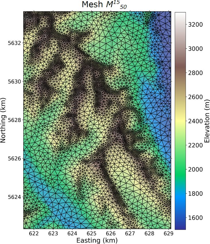
744                                   V. Vionnet et al.: Multi-scale snowdrift-permitting modelling of mountain snowpack

the snow accumulation and ablation periods at a large range       et al., 2020a). These models can be classified as snowdrift-
of spatial scales (e.g., Pomeroy and Gray, 1995; Pomeroy          permitting models since they operate at sufficient resolutions
et al., 1998, 2012, 2016; Clark et al., 2011; Mott et al.,        (200 m or finer) to activate the horizontal redistribution of
2018). Snow accumulation at the mountain range scale (1–          snow between computational elements. High-resolution re-
500 km) is primarily dominated by orographic precipitation        mote sensing data assimilation can also be used at these
and results in regions of enhanced or reduced snowfall (e.g.,     scales to correct spatial biases in the atmospheric forcing and
Houze, 2012). At the mountain ridge and slope scales (5 m–        to account for missing physical processes in the models (e.g.,
1 km), preferential deposition of snowfall and blowing-snow       Durand and Margulis, 2008; Baba et al., 2018).
transport, including transport in both saltation and suspen-         Snowdrift-permitting models simulate wind-induced snow
sion layers, strongly impact snow accumulation (e.g., Mott et     transport in the saltation and suspension layers (e.g, Pomeroy
al. 2018). Redistribution by avalanches (e.g., Bernhardt and      and Gray, 1995). As proposed by Mott et al. (2018), they
Schulz, 2010; Sommer et al., 2015) and surface and blowing-       can be divided into two main categories: (i) models solv-
snow sublimation (e.g., MacDonald et al., 2010; Vionnet et        ing the vertically integrated mass flux in the saltation and
al., 2014; Musselman et al., 2015; Sextone et al., 2018) also     suspension layers (Essery et al., 1999; Durand et al., 2005;
modify the spatial variability of snow. During the ablation       Pomeroy et al., 2007; Liston et al., 2007) and (ii) mod-
period, spatially varying melt rates result from differences      els solving the three-dimensional (3-D) advection-turbulent
in solar irradiance due to aspect and shading (e.g., Marks        diffusion equation of blown snow particles in the atmo-
and Dozier, 1992; Marsh et al., 2012), in net solar irradiance    sphere (Gauer, 1998; Lehning et al., 2008; Schneiderbauer
due to albedo variations (e.g., Dumont et al., 2011; Schirmer     and Prokop, 2011; Sauter et al., 2013; Vionnet et al., 2014).
and Pomeroy, 2020), in turbulent fluxes (e.g., Winstral and       One of the main challenges for all these models is obtain-
Marks, 2014; Gravelman et al., 2015) and in advected heat         ing accurate driving wind fields at sufficient high resolution
from snow-free ground in patchy snow cover conditions (e.g.,      since they strongly impact the accuracy of simulated snow
Mott et al., 2013; Harder et al., 2017; Schlögl et al., 2018).    redistribution (Mott and Lehning, 2010; Musselman et al.,
   The multi-scale variability of mountain snow represents        2015). Models of the first category need two-dimensional
a challenge for snow models used in support of avalanche          (2-D) driving wind fields. Liston et al. (2007), inspired by
hazard forecasting (Morin et al., 2020), hydrological pre-        Ryan (1977), proposed the use of terrain-based parameters
dictions (e.g., Warscher et al., 2013; Brauchli et al., 2017;     to adjust distributed wind fields to the local topography.
Freudiger et al., 2017) and climate projections (e.g., Rasouli    These distributed wind fields can be obtained from interpo-
et al., 2014; Hanzer et al., 2018) in mountainous terrain. Sev-   lated station data (Gascoin et al., 2013; Sextone et al., 2018),
eral modelling strategies have been proposed to face this         hourly output from regional climate models at a convective-
challenge and to capture this multi-scale variability. At the     permitting scale (Reveillet et al., 2020) or a pre-computed
mountain range scale, atmospheric models at sufficient res-       wind field library using an atmospheric model (Berhnardt
olutions (4 km or finer) can provide valuable information on      et al., 2010). Essery et al. (1999) used a linearized turbu-
the variability of snowfall and resulting snow accumulation       lence model (Walmsley et al., 1982) to build a pre-computed
(e.g., Prein et al., 2015; Lundquist et al., 2019; Fang and       library of 2-D wind maps to distribute wind measurements
Pomeroy, 2020). Indeed, at these resolutions, atmospheric         from station data. Musselman et al. (2015) showed that this
models operate at convection-permitting scales and explicitly     approach led to more accurate simulations of snow redistri-
represent convection and highly resolved vertical motions,        bution around an alpine crest than wind fields derived from
achieving improved estimates of snowfall (e.g., Rasmussen         the terrain-based parameters proposed by Liston et al. (2007).
et al., 2011). Sub-grid parameterizations of snow depth have      Models of the second category require a 3-D representation
been proposed to represent the snow variability at the moun-      of the wind field and associated atmospheric turbulence. In
tain ridge and slope scale for snowpack models operating at       this case, driving wind fields can be obtained from compu-
kilometre scales (Liston, 2004; Helbig and van Herwijnen,         tational fluid dynamics (CFD) models (Gauer, 1998; Schnei-
2017; He and Ohara, 2019). Another strategy consists of ex-       derbauer and Prokop, 2011) or atmospheric models in large-
plicitly modelling the snow evolution at the mountain ridge       eddy simulation (LES) mode used to generate a library of
and slope scales at resolutions ranging from a few metres         pre-computed wind fields (Lehning et al., 2008; Mott and
to 200 m (Liston, 2004; Musselman et al., 2015). At these         Lehning, 2010) or fully coupled to a snowpack model (Vion-
scales, the variability of snow accumulation can be repre-        net et al., 2014). These advanced models can be used for de-
sented using (i) simple parameterizations to adjust snowfall      tailed studies such as the feedbacks between blowing-snow
as a function of topographic parameters (e.g., Winstral and       sublimation and the atmosphere (Groot Zwaaftink et al.,
Marks, 2002; Hanzer et al., 2016) or (ii) models that explic-     2011) or the processes driving the variability of snow accu-
itly represent preferential deposition and/or wind-induced        mulation during a snowfall event, including preferential de-
snow redistribution (e.g., Essery et al., 1999; Durand et al.,    position of snowfall (Lehning et al., 2008; Mott et al., 2010;
2005; Pomeroy et al., 2007; Liston et al., 2007; Lehning et       Vionnet et al., 2017).
al., 2008; Sauter et al., 2013; Vionnet et al., 2014; Marsh

The Cryosphere, 15, 743–769, 2021                                                      https://doi.org/10.5194/tc-15-743-2021
V. Vionnet et al.: Multi-scale snowdrift-permitting modelling of mountain snowpack                                         745

   Differences in the level of complexity of snowdrift-          full winter around the Kananaskis Valley in the Canadian
permitting models and associated driving wind fields influ-      Rockies. Different model configurations were tested to as-
ence the spatial and temporal ranges of application of these     sess the impact of the representation of physical processes
models. Due to their relatively low computational costs,         in CHM as well as the complexity of the wind-downscaling
models of the first category can be applied to simulate the      scheme. Airborne lidar snow depth data and snow persis-
snow cover evolution over entire snow seasons at a res-          tence indexes derived from Sentinel-2 images were used
olution between 25 and 200 m for regions covering hun-           to evaluate the ability of the different CHM configurations
dreds of square kilometres (e.g., 210 km2 for Berhnardt et       to capture the elevation–snow depth relationship as well as
al., 2010; 1043 km2 for Gascoin et al., 2013; 3600 km2 for       snow redistribution around wind-exposed ridges. The pa-
Sextone et al., 2018). On the other hand, models of the sec-     per is organized as follows: Sect. 2 presents the study area
ond category are usually restricted to the simulation of sin-    and the different observation datasets used in this study, and
gle blowing-snow events at resolution between 2 m and 50 m       it also describes the CHM modelling platform, the wind-
over regions covering tens of square kilometres (e.g., 1 km2     downscaling strategy and the configurations of the CHM ex-
in Schneiderbauer and Prokop, 2011, 2.3 km2 in Mott and          periments. Section 3 evaluates the impact of the wind field
Lehning, 2010; 23 km2 in Vionnet et al., 2017). The study        downscaling and the quality of the snowpack simulations us-
by Groot Zwaaftink et al. (2013) is an exception and relied      ing airborne lidar snow depth data and snow persistence in-
on the Alpine 3D model (Lehning et al., 2008) to simulate        dexes; Sect. 4 discusses the main challenges associated with
the snow cover evolution at 10 m resolution over a region        snowdrift-permitting modelling of mountain snowpack and
of 2.4 km2 of the Swiss Alps for an entire winter. All these     associated limitations. Finally, concluding remarks are pre-
snowdrift-permitting models used a gridded representation        sented in Sect. 5.
of the topography. Large-scale applications of these mod-
els over mountainous area are limited by the need to have
a fixed and sufficiently high resolution over large areas even   2     Data and methods
in regions where wind-induced snow transport is not active
(valley bottom for example).                                     2.1     Study site
   To overcome some of these limitations, Marsh et al.
                                                                 This work studies the evolution of the mountain snowpack
(2020a) developed a snowdrift-permitting scheme of inter-
                                                                 around the Kananaskis Valley of the Canadian Rockies, Al-
mediate complexity that solves the 3-D advection–diffusion
                                                                 berta (Fig. 1). The study domain covers an area of 958 km2
blowing-snow transport on a variable resolution unstructured
                                                                 and is characterized by a complex and rugged topography
mesh. This scheme is implemented in the Canadian Hy-
                                                                 with elevations ranging from 1400 m at the Kananaskis Val-
drological Model (CHM; Marsh et al., 2020b). The land-
                                                                 ley bottom in the northeastern part of the domain up to
scape is discretized using a variable resolution unstructured
                                                                 3406 m at the summit of Mount Sir Douglas in the southern
mesh that allows an accurate representation of terrain hetero-
                                                                 part of the region (Fig. 1b). Valley bottoms and lower slopes
geneities with limited computation elements (Marsh et al.,
                                                                 are predominately covered by needleleaf evergreen forest
2018). Marsh et al. (2020a) used the WindNinja diagnostic
                                                                 (Fig. 1a). Short shrubs and low vegetation are present near
wind model (Forthofer et al., 2014) to build libraries of pre-
                                                                 treeline whereas exposed rock surfaces, talus and grasses are
computed wind fields. Wagenbrenner et al. (2016) showed
                                                                 found in the highest alpine elevations. The Kananaskis Val-
that WindNinja can be used to downscale wind field from at-
                                                                 ley hosts several meteorological stations that are part of the
mospheric models running at a convection-permitting scale
                                                                 University of Saskatchewan’s Canadian Rockies Hydrolog-
in complex terrain.
                                                                 ical Observatory (CRHO; https://research-groups.usask.ca/
   The objective of the present study is to develop and evalu-
                                                                 hydrology/science/research-facilities/crho.php, last access:
ate a novel strategy for multi-scale modelling of mountain
                                                                 29 January 2021) and is active for research in snow hy-
snowpack over large regions and for entire snow seasons.
                                                                 drology (e.g., MacDonald et al., 2010; Musselman et al.,
Specifically, the following questions are asked. (1) Can effi-
                                                                 2015; Pomeroy et al., 2012; 2016; Fang et al., 2019; Fang
cient wind-downscaling approaches be used for blowing sim-
                                                                 and Pomeroy, 2020). More details about these meteorologi-
ulation? (2) Over large spatial extents, can lateral mass re-
                                                                 cal stations are given in Sect. 2.3.1.
distribution (blowing snow and avalanching) be ignored? (3)
Can optical satellite imagery be used to diagnose model per-     2.2     Model
formances over large spatial extents? This modelling strat-
egy combines (i) atmospheric forcing from the convection-        2.2.1    Mesh generation
permitting Canadian numerical weather prediction (NWP)
system, (ii) a downscaling module including wind fields from     The digital elevation model (DEM) from the Shuttle Radar
a high-resolution diagnostic wind model and (iii) the multi-     Topography Mission-SRTM (EROS Center, 2017) at a reso-
scale snowdrift-permitting model CHM running on an un-           lution of 1 arcsec (30 m) was used as input to the mesher code
structured mesh. This modelling strategy was applied for a       (Marsh et al., 2018) to generate an unstructured, variable-

https://doi.org/10.5194/tc-15-743-2021                                                    The Cryosphere, 15, 743–769, 2021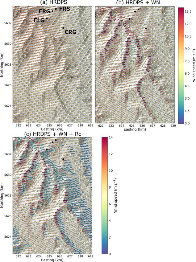
746                                      V. Vionnet et al.: Multi-scale snowdrift-permitting modelling of mountain snowpack

Figure 1. (a) Land cover map and (b) elevation map of the Kananaskis Valley, Alberta, Canada, study domain. The glacier mask is taken
from the Randolph Glacier Inventory version 6.0 (Pfeffer et al., 2014). The red-shaded area corresponds to the area shown in Figs. 2, 3, 6
and 10. The characteristics of the meteorological stations are given in Table 3. Areas labelled from 1 to 3 correspond to sub-regions used in
the analysis of the results (see Sect. 2.3.2).

resolution triangular mesh over the Kananaskis domain                    Marks, 2005; Pomeroy et al., 2016; Hedrick et al., 2018).
(Fig. 1). In mesher, triangles are bounded with minimum and              Snobal is a physically based snowpack model that approxi-
maximum areas and are generated to fulfil a given tolerance              mates the snowpack with two layers. The surface layer was
defined here as the root-mean-square error to the underlying             implemented here with a fixed thickness of 0.1 m and is used
topographic raster. This study uses a high-resolution mesh,              to estimate surface temperature for outgoing longwave ra-
denoted M50  15 with a minimum triangle area of 50 m × 50 m              diation and turbulent heat fluxes. The second lower layer
and a vertical tolerance of 15 m. The characteristics of the             represents the remaining snowpack. For each layer, Snobal
generated mesh are given in Table 1. For the Kananaskis do-              simulates the evolution of the snow water equivalent (SWE),
main, 383 200 raster grid cells with a 50 m resolution are               temperature, density, cold content and liquid water content.
required to represent the terrain, whereas 101 700 triangles             The version of Snobal used in this study includes an im-
are used in M50 15 (Fig. 2). Large triangles are found in valley         proved algorithm for snow compaction that accounts for bulk
bottoms of low topographic variability, whereas small trian-             compaction and temperature metamorphism (Hedrick et al.,
gles dominate in alpine terrain, close to ridges where wind-             2018). Snobal in CHM employs the snow albedo routine of
induced snow redistribution is common.                                   Verseghy et al. (1993). The ground heat flux assumes heat
   A dataset of tall vegetation (> 5 m) coverage, with a res-            flow to a single soil layer of known temperature and thermal
olution of 30 m (Fig. 1a), was obtained from Hansen et al.               conductivity. In these simulations, the soil temperature was
(2013). These fractional values were applied to the triangular           set to −4 ◦ C at 10 cm below the soil–snow interface. Marsh
mesh via mesher by averaging the raster cells that correspond            et al. (2020b) used the same value for Snobal simulations
to each triangle and assigning this average to the triangle. Tri-        with CHM at the Marmot Creek Research Basin located fur-
angles with an average fraction of high vegetation larger than           ther north in the Kananaskis Valley (Fig. 1).
0.5 were classified as forest.                                              CHM also includes a 3-D advection–diffusion blowing-
                                                                         snow transport and sublimation model (Marsh et al., 2020a):
2.2.2   Snowpack model                                                   the 3-D Prairie Blowing Snow Model (PBSM-3D). This
                                                                         scheme uses a finite-volume method discretization on the un-
Distributed snowpack simulations over the triangular mesh                structured mesh. It deploys the parameterization of Li and
of the study area were performed using the version of the                Pomeroy (1997) to determine the threshold wind speed for
Snobal scheme (Marks et al., 1999) implemented in CHM                    snow transport initiation as a function of air temperature and
(Marsh et al. 2020b). Snobal has been used in numerous                   snow presence. It does not depend on the properties of sur-
mountainous regions across North America (e.g., Garen and

The Cryosphere, 15, 743–769, 2021                                                              https://doi.org/10.5194/tc-15-743-2021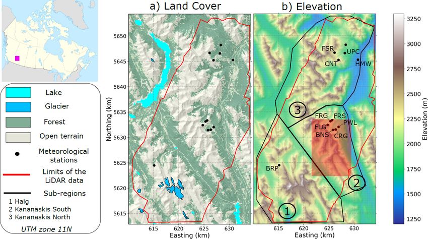
V. Vionnet et al.: Multi-scale snowdrift-permitting modelling of mountain snowpack                                                       747

Table 1. Characteristics of the mesh used in this study. The vertical error corresponds the root-mean-square error to the underlying reference
topographic raster.

                  Name of      Minimum triangle      Maximum triangle      Median triangle     Vertical error   Number of
                  the mesh        area (m2 )            area (m2 )           area (m2 )             (m)          triangles
                   15
                  M50               50 × 50              250 × 250             63 × 63              15           101 700

                                                                         concentration of blowing-snow particles accounting for ad-
                                                                         vection, turbulent diffusion, sedimentation and mass loss due
                                                                         to sublimation based on the parameterizations proposed by
                                                                         Pomeroy and Male (1992) and Pomeroy et al. (1993). At a
                                                                         given time step, erosion and deposition rates are computed as
                                                                         the spatial divergence of the saltation and suspension fluxes,
                                                                         and the snowpack simulated by Snobal is updated accord-
                                                                         ingly. In this study, 10 layers were used for a total height of
                                                                         the suspension layer of 5 m as in Marsh et al. (2020a). Snow-
                                                                         fall over complex terrain is calculated by GEM according
                                                                         to its microphysics scheme (Milbrandt et al., 2016). CHM
                                                                         does not simulate explicitly preferential deposition of snow-
                                                                         fall (Lehning et al., 2008; Mott et al., 2018). New snow is
                                                                         added to the surface layer in Snobal and, if wind speeds ex-
                                                                         ceed the threshold wind speed, it is transported in the salta-
                                                                         tion and suspension blowing-snow layers by PBSM-3D.
                                                                            In steep alpine terrain, gravitational snow transport
                                                                         strongly affects the spatial variability of the snowpack (e.g.,
                                                                         Sommer et al., 2015) and the mass balance of glaciers
                                                                         (Mott et al., 2019) and modifies the runoff behaviour of
                                                                         alpine basins (Warscher et al. 2013). For these reasons, the
                                                                         SnowSlide scheme (Bernhard and Schulz, 2010) was im-
                                                                         plemented in CHM. SnowSlide is a simple topographically
                                                                         driven model that simulates the effects of gravitational snow
Figure 2. Variable-resolution triangular mesh used in this study
                                                                         transport. SnowSlide uses a snow-holding depth that de-
over a sub-area of the Kananaskis domain. The location of this sub-      creases exponentially with increasing slope angle, limiting
area corresponds to the red-shaded area shown in Fig. 1b. The un-        snow accumulation in steep terrain. SnowSlide was initially
derlining DEM was taken from the SRTM mission at 1 arcsec.               developed for regular gridded rasters and has been adapted
                                                                         here to the unstructured triangular mesh used by CHM.
                                                                         SnowSlide operates from the highest triangle of the mesh to
face snow (e.g., density, liquid water content) simulated by             the lowest one. If the snow depth exceeds the snow-holding
Snobal (see Sect. 4.4 for a discussion on the limitation of              capacity for a given triangle, excess snow is redistributed to
this approach). In the case of blowing-snow occurrence, the              the lower adjacent triangles, proportionally to the elevation
steady-state saltation parameterization of Pomeroy and Gray              difference between the neighbouring triangles and the origi-
(1990) is used to compute the mass concentration in the salta-           nal one. SnowSlide uses the total elevation (snow depth plus
tion layer. The concentration in the saltation layer is impacted         surface elevation) to operate. In this study, the default formu-
by shear stress partitioning due to the presence of vegetation           lation of the snow-holding depth proposed by Bernhardt and
(such as shrubs) and the upwind fetch. Upwind fetch is cal-              Schulz (2010) is used, which leads to a maximal snow thick-
culated for each triangle of the mesh using the fetchr param-            ness (taken perpendicular to the slope) of 3.08 m, 1.11 m,
eterization of Lapen and Martz (1993) and is used to reduce              0.45 m and 0.15 m for slopes of 30◦ , 45◦ , 60◦ and 75◦ , re-
the mass concentration in the saltation layer in regions where           spectively.
flow is developing. The saltation layer acts as a lower bound-              The impact of the presence of forest vegetation on snow
ary condition for the suspension layer, which is discretized             interception, sublimation, snowpack accumulation and melt
with a user-defined number of layers to resolve the gradient             energetics is represented in CHM using the same canopy
of concentration of blowing-snow particles in the suspension             module as in the Cold Region Hydrological Model (CRHM;
layer. For each layer, PBSM-3D solves the evolution of the               Ellis et al., 2010; Pomeroy et al. 2012). This module used leaf

https://doi.org/10.5194/tc-15-743-2021                                                              The Cryosphere, 15, 743–769, 2021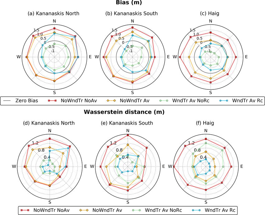
748                                  V. Vionnet et al.: Multi-scale snowdrift-permitting modelling of mountain snowpack

area index and canopy closure to compute the effect of forests   taken from the HRDPS forecast, and direct irradiance was
on shortwave and longwave irradiance at the snow surface.        corrected for slope and aspect as described in Marsh et al.
Snow interception and sublimation of intercepted snow are        (2012). Local terrain shadowing and its impact on shortwave
also represented following Hedstrom and Pomeroy (1998).          irradiance were calculated using the algorithm of Dozier and
In this study, the canopy module was activated for the trian-    Frew (1990) adapted for unstructured meshes as described
gles covered by forest as described in Sect. 2.2.1.              in Marsh et al. (2020b). Longwave irradiance was adjusted
                                                                 for elevation difference using the climatological lapse rate of
2.2.3   Atmospheric forcing                                      Marty et al. (2002). Finally, wind speed and direction were
                                                                 taken from the lowest HRDPS prognostic level at 40 m above
Snobal and PBSM-3D require the following atmospheric             the surface and were downscaled to the CHM mesh using the
forcing: air temperature, humidity, wind speed, wind di-         strategy described in the next section.
rection, liquid and solid precipitation rates, and longwave
and shortwave irradiance. Due to the scarcity of the net-        2.2.4   Wind field downscaling
work of meteorological stations in the region (Fig. 1),
hourly atmospheric forcings were obtained from the High-         Mountain wind fields are notoriously difficult to observe and
Resolution Deterministic System (HRDPS; Milbrandt et al.,        model (Davies et al., 1995), and obtaining high-resolution
2016). HRDPS is the high-resolution NWP system running           wind fields constitutes one of the greatest challenges for
the Global Environmental Multiscale Model (GEM) oper-            blowing-snow models in mountainous terrain (e.g., Mott and
ationally over Canada at 2.5 km grid spacing. Successive         Lehning, 2010; Vionnet et al., 2014; Musselman et al., 2015;
HRDPS forecasts from the 00:00 and 12:00 UTC analysis            Réveillet et al., 2020). In the context of this study, hourly
time at 6 to 17 h lead time were extracted over the region       HRDPS near-surface wind fields at the 2.5 km scale were
and combined together to generate a continuous atmospheric       downscaled to the CHM mesh over the full duration of the
forcing. Previous studies have also used distributed forcing     simulations (1 water year). This required a computationally
data from NWP systems to drive snowpack models in moun-          efficient wind-downscaling method. Therefore, the wind-
tainous terrain since these data can often represent the com-    downscaling strategy used in this study was derived from
plex interactions between topography and atmospheric flow        the method proposed by Barcons et al. (2018) for mesoscale-
better than sparse meteorological measurements (Quéno et         to-microscale downscaling of near-surface wind fields. This
al., 2016; Vionnet et al., 2016; Havens et al. 2019; Lundquist   method combines precomputed microscale simulations with
et al., 2019; Fang and Pomeroy, 2020).                           a mesoscale forecast using transfer functions. In their study,
   The HRDPS atmospheric forcing at 2.5 km grid spacing          Barcons et al. (2018) combined the Weather Research and
was downscaled to the triangles of the CHM mesh. Hori-           Forecast mesoscale model at 3 km grid spacing and the Alya-
zontal interpolation was first applied using inverse-distance    CFDWind microscale model at 40 m grid spacing. In our
weighting from the closest four HRDPS grid points. Cor-          study, microscale wind simulations were generated with the
rections for elevation differences were then applied to adapt    WindNinja model. WindNinja is a mass-conserving diag-
the HRDPS meteorological forcing to the high-resolution to-      nostic wind model, primarily designed to simulate mechan-
pography of the CHM mesh. Constant monthly lapse rates           ical effects of terrain on the flow (Forthofer et al., 2014).
were used to adjust HRDPS 2 m air temperature and humid-         Forthofer et al. (2014) showed that the model captures impor-
ity (Kunkel, 1989; Shea et al., 2004). HRDPS temperature         tant terrain-induced flow features, such as ridgetop accelera-
was reduced (increased) if the elevation of the triangle is      tion or terrain channelling, and can improve wildfire spread
higher (lower) than the elevation of the HRDPS grid points.      predictions in complex terrain. Wagenbrenner et al. (2016)
Precipitation amounts were not modified to account for ele-      used the model to directly downscale near-surface wind fore-
vation difference as it was assumed that HRDPS already cap-      casts from NWP systems in complex terrain.
tures the main orographic effects affecting mountain precip-        The application and extension of the Barcons et al. (2018)
itation (Lundquist et al., 2019). The precipitation adjustment   approach for use on an unstructured mesh and to account
function of Liston and Elder (2006) has been tested but it       for direction perturbations are detailed below. First, to build
led to strong overestimation of snow depth at high elevation     the wind map library, WindNinja was run at 50 m resolu-
(not shown), suggesting that this factor may not be adapted      tion over the Kananaskis domain (Fig. 1). As WindNinja
to account for the subgrid variability of precipitation amount   uses a regular grid, the input topography was taken from
within a 2.5 km grid. A cosine correction was then applied to    the same SRTM DEM at 30 m grid spacing that was used
adjust precipitation falling on an inclined triangle for mass-   to build the CHM mesh (Sect. 2.2.1). WindNinja used a spa-
conservation purposes (Kienzle, 2011). Downscaled temper-        tially constant roughness length (z0 = 0.01 m) representative
ature and humidity were finally used to compute the precip-      of snow-covered terrain in alpine topography (Mott et al.,
itation phase with the psychrometric energy balance method       2010; Mott and Lehning, 2010), and vegetation effects were
of Harder and Pomeroy (2013) that performed well in the          introduced later in the downscaling procedure, as described
Kananaskis Valley. Direct and diffuse solar irradiance were      below. WindNinja simulations were carried out for 24 initial

The Cryosphere, 15, 743–769, 2021                                                    https://doi.org/10.5194/tc-15-743-2021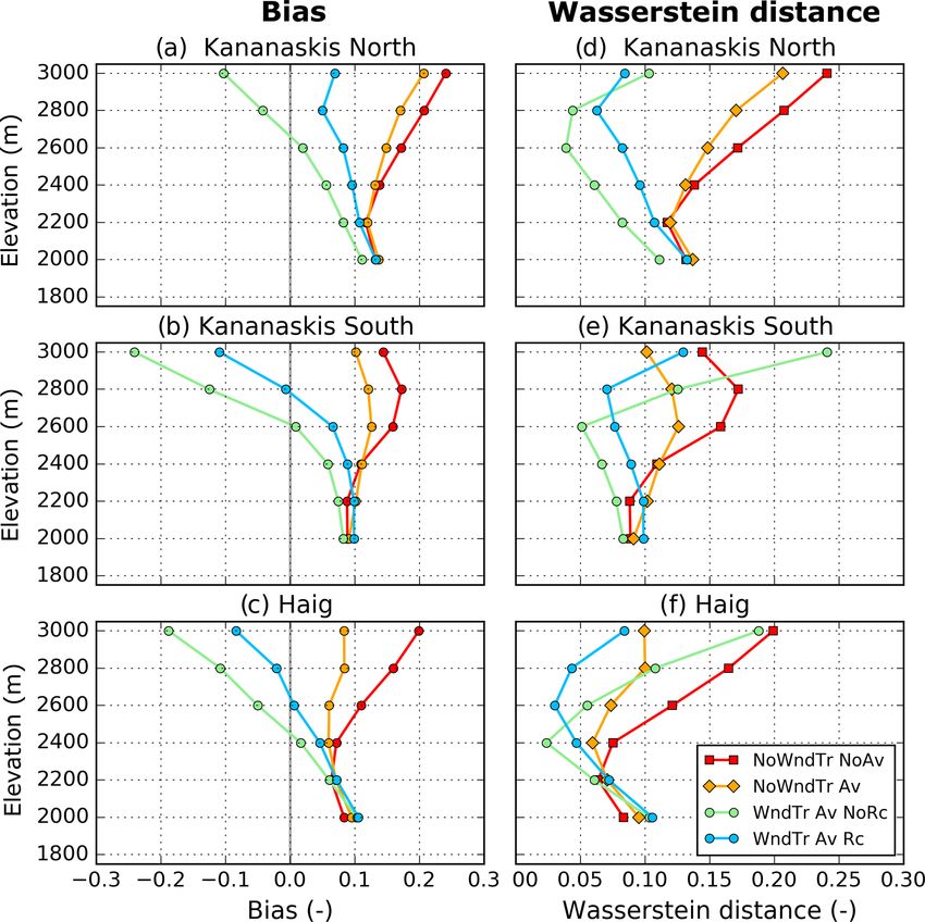
V. Vionnet et al.: Multi-scale snowdrift-permitting modelling of mountain snowpack                                           749

wind directions (each 15◦ ) with an initial wind speed at 40 m     cover of the triangle as defined in Sect. 2.2.1. Fetch effects
above the surface set to 10 m s−1 . The height of 40 m corre-      due to the presence of upstream vegetation are not taken into
sponds to the lowest HRDPS prognostic level.                       account when adjusting the wind speed.
   Then, for each wind direction in the wind map library, the         Forthofer et al. (2014) and Wagenbrenner et al. (2016,
transfer function f was computed for use in the downscaling        2019) showed that the mass-conserving version of Wind-
procedure given as                                                 Ninja has difficulties simulating lee-side recirculation where
                                                                   flow separation occurs. This difficulty is due to the absence
      UWN                                                          of a momentum equation in the WindNinja flow simulation
f=           ,                                              (1)
     hUWN iL                                                       (Forthofer et al., 2014). As lee-side flow strongly influences
                                                 q                 snow accumulation (e.g., Gerber et al., 2017), an additional
where UWN is the local wind speed (UWN = u2WN + vWN        2 ),    and optional step was added to the wind-downscaling proce-
uWN and vWN are the horizontal components of the wind at           dure described above. It consisted of a modification of the
50 m resolution, and hUWN iL is the spatial average of UWN         transfer functions fdown to reduce wind speed in leeward ar-
over an area of size L × L. By construction, when L tends          eas prone to flow separation. At each CHM time step, lee-
towards 0, f tends towards 1. As L increases, f incorporates       ward areas were identified using the Winstral topographic pa-
the local wind fluctuation induced by the microscale terrain       rameter Sx (Winstral and Marks, 2002; Winstral et al., 2017),
features (Barcons et al., 2018). A value of L = 1000 m was         computed at each triangle using the downscaled wind direc-
used in this study in agreement with the finding of Barcons et     tion, θDown . The Sx algorithm examines all triangles along a
al. (2018) in complex terrain. Note that Barcons et al. (2018)     fixed search line emanating from the triangle of interest to
used a circle instead of a square to compute the spatial aver-     determine which triangle has the greatest upward slope rel-
age of the wind speed. Thus, f acts as a speedup/slowdown          ative to the triangle of interest. Positive Sx values indicate
factor that accounts for topographic impacts on wind speed.        sheltering features whereas negative Sx values indicate that
Only one value for the initial wind speed was used to build        the triangle of interest height is the highest cell along the
the wind library due to the insensitivity of the transfer func-    search line and is topographically exposed. In this study, the
tion to the initial wind speed found with WindNinja.               Sx algorithm used a search distance of 300 m, as in Winstral
   To account for impacts on direction, the following ap-          et al. (2017). Triangles with Sx values larger than 20◦ were
proach was taken. The rasters of the wind map library con-         considered susceptible to flow separation in agreement with
taining the horizontal u and v wind components and the             previous studies on the onset of flow separation in complex
transfer function f for each initial wind direction were ap-       terrain (e.g., Wood, 1995). For these triangles, the transfer
plied to the triangles of the unstructured mesh using the          function, fdown , was set to a value of 0.25 (Winstral et al.,
mesher code (Marsh et al., 2018). At each CHM time step,           2009). Note finally that a mass- and momentum-conserving
the HRDPS uHRDPS and vHRDPS wind components were spa-              version of WindNinja is also available (Wagenbrenner et al.,
tially interpolated to the triangles’ centres with an inverse-     2019). Wagenbrenner et al. (2019) have shown that momen-
distance interpolant using the four closest HRDPS grid             tum conservation improved flow simulation at windward and
points. For each triangle, the interpolated HRDPS wind di-         leeward locations compared to the mass-conserving version,
rection, θHRDPS , was then reconstructed from the interpolated     but numerical instabilities made this version of the code un-
HRDPS wind components, uHRDPS_int and vHRDPS_int . This            usable in the complex topography of the Canadian Rockies.
direction was used to select the two sets of precomputed mi-
croscale wind components with the wind directions ϕ1 and           2.2.5   Model experiments
ϕ2 that bound θHRDPS (i.e., ϕ1 < θHRDPS < ϕ2 ). These se-
lected microscale wind components including the local ter-         A set of CHM experiments were designed to assess the ef-
rain effect were then linearly interpolated and recombined         fect of the wind field downscaling and the impact of pro-
to obtain the downscaled wind direction θDown . The trans-         cess representation on snowpack simulations at snowdrift-
fer functions corresponding to the wind directions ϕ1 and ϕ2       permitting scales (Table 2). A reference CHM configura-
were also linearly combined to obtain the final transfer func-     tion including wind downscaling accounting for recircula-
tion, fdown . It was finally applied to scale the modulus of the   tion and gravitational and blowing-snow redistribution was
interpolated HRDPS wind speed and derive the final down-           first defined (WndTr Av Rc). A stepwise model falsification
scaled wind speed as in Barons et al. (2018):                      was then used, removing the following processes from the
                                                                   model: (i) recirculation effects in the wind-downscaling pro-
             q                                                     cedure (WndTr Av NoRc), (ii) blowing-snow redistribution
UDown = fdown u2HRDPS_int + vHRDPS_int
                             2         .                    (2)    with PBSM-3D (NoWndTr Av), (iii) gravitational snow redis-
                                                                   tribution with SnowSlide (NoWndTr NoAv), (iv) wind down-
   Wind speeds were then adjusted to 10 m wind speeds using        scaling with WindNinja (NoDown). Note that all the CHM
the Prandtl–von Kármán logarithmic wind profile and mod-           experiments considered in this study account for the effects
ified to include vegetation interactions using the vegetation      of terrain slope and aspect on incoming shortwave radiation.

https://doi.org/10.5194/tc-15-743-2021                                                    The Cryosphere, 15, 743–769, 2021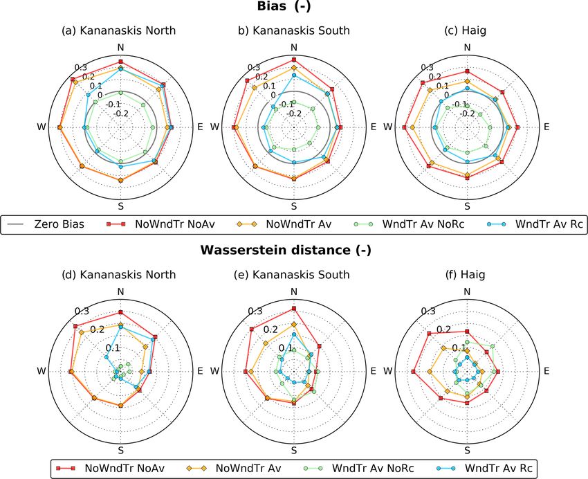
750                                    V. Vionnet et al.: Multi-scale snowdrift-permitting modelling of mountain snowpack

These simulations covered the period from 1 September 2017          files, and LAStools (https://rapidlasso.com/lastools/, last ac-
to 31 August 2018 to fully capture snow accumulation and            cess: 29 January 2021) was used to generate 5 m resolu-
ablation in the region. For each experiment, CHM outputs            tion digital elevation models (DEMs). The summer and win-
were rasterized to a 50 m × 50 m raster for model evaluation.       ter DEMs were co-registered to minimize slope and aspect-
This rasterization was done via the GDAL rasterization ca-          induced errors (Nuth and Kääb, 2011). Additional details
pabilities (GDAL/OGR contributors, 2020). In short, this al-        about the processing workflow over snow-covered terrain can
gorithm takes the triangle geometry in conjunction with an          be found in Pelto et al. (2019). To estimate uncertainties
output raster (with given cell sizes and domain extent) and         on the snow depth retrieval, snow-free areas that included
resolves which raster cells correspond to each triangle. In the     peaks and road surfaces were identified in a 3 m satellite im-
case that two triangles share an output cell, an overwrite is       agery (Planet Scope) for 27 April 2018. Analysis of eleva-
used by the algorithm. The 50 m × 50 m area was selected as         tion change over these snow-free surfaces (34 comparison
it corresponds to the minimal triangle area for high resolution     points across all elevation) indicated an average (median) el-
used in this study (Table 1).                                       evation change of −4.1 cm (0.5 cm) and a standard deviation
                                                                    of 19.8 cm. The median absolute deviation reached 8.0 cm.
2.3     Data and evaluation methods                                 The DEM of snow depth was masked to only include non-
                                                                    glacierized terrain (Fig. 1b) and to exclude any areas of ele-
2.3.1    Meteorological observations                                vation change that was less than 0 m and greater than 20 m;
                                                                    elevation change beyond these values is considered an out-
Hourly meteorological data collected at CRHO stations were          lier (Grünewald et al., 2014) and can arise from steep terrain
used to evaluate the precipitation and wind fields driving          that was effectively in the shadow of the laser scanner. For
CHM (Table 3). These stations include those in Marmot               model evaluation, the 5 m snow depth map was then resam-
Creek Research Basin (Fang et al., 2019) and Fortress Moun-         pled over the same 50 m raster as the CHM output, taking
tain Snow Laboratory (Harder et al., 2016) (Table 3 and             for each cell of the 50 m raster the average of all non-masked
Fig. 1), covering an elevation range from 1492 to 2565 m.           cells in the 5 m snow depth map. Cells of the 50 m raster that
Table 3 also provides the topographic position index (TPI) at       contained more than 75 % of masked cells in the 5 m snow
the position of the stations (Table 3) as this metric provides      depth map were masked out. In addition, grid points cov-
a quantification of each station’s elevation relative to its sur-   ered by glaciers identified in the Randolph Glacier Inventory
roundings. In this study, TPI was defined as in Winstral et al.     (Pfeffer et al., 2014) were removed from the analysis since
(2017) and consists of the difference between each station’s        elevation change over these surfaces is also influenced by ice
elevation on a 50 m raster minus the mean of all pixel eleva-       dynamics (Pelto et al., 2019). Finally, forested pixels identi-
tions located within a 2 km radius from the station. Hourly         fied using the global database of Hansen et al. (2013) at 30 m
meteorological data were obtained from quality-controlled           grid spacing were masked out as well since this study focuses
15 min observations using the same method as in Fang et al.         on snow redistribution processes in open terrain.
(2019). In particular, solid precipitation data were corrected         The distributions of simulated and observed snow depths
from wind-induced undercatch using the method proposed              were compared for different 200 m elevation bands for three
by Smith (2007). Simulated wind speeds were corrected to            sub-areas of the Kananaskis domain (Fig. 1b): (i) Kananaskis
the sensor height of each station (including snow depth) us-        North, (ii) Kananaskis South and (iii) Haig. These three
ing a standard log-law for the vertical profile of wind speed       sub-areas were characterized by a different mean (standard
near the surface and an aerodynamic roughness of 1 mm typi-         deviation) of observed snow depths: 0.90 m (0.82 m) for
cally found in snow-covered alpine terrain (e.g., Naaim Bou-        Kananaskis North, 1.32 m (1.03 m) for Kananaskis South and
vet et al., 2010).                                                  2.00 m (1.33 m) for Haig. For each elevation band, the root-
                                                                    mean-squared error (RMSE) and the Wasserstein distance of
2.3.2    Airborne lidar snow depth data                             order 1, W1 (Rüschendorf, 1985), were used to quantify the
                                                                    agreement between the simulated and the observed distribu-
Airborne laser scanning (ALS) surveys were performed over           tions. W1 is defined as
the Kananaskis region on 5 October 2017 (late summer                            Z+∞
scan) and on 27 April 2018 (winter scan) using a Riegl Q-
                                                                    W1 (s, o) =    |S(s) − O(o)| ,                             (3)
780 infrared (1024 nm) laser scanner with a dedicated Ap-
planix POS AV Global Navigation Satellite System (GNSS)                        −∞

inertial measurement unit (IMU). The Q-780 scanner was              where s and o are the simulated and observed snow depth
flown at heights of approximately 2500 m above the ter-             distributions and S and O the corresponding cumulative dis-
rain that yielded swath widths of 2000 to 3000 m. Post-             tribution functions. W1 has the same unit as the variable con-
processing of the ALS survey flight trajectory yielded verti-       sidered (here metres for snow depth), d and a perfect match
cal and horizontal positional uncertainties of ±15 cm (1σ ).        between the distribution led to W1 = 0. For each sub-area,
Post-processed point cloud data were exported into LAS              simulated and observed snow depth distributions were also

The Cryosphere, 15, 743–769, 2021                                                       https://doi.org/10.5194/tc-15-743-2021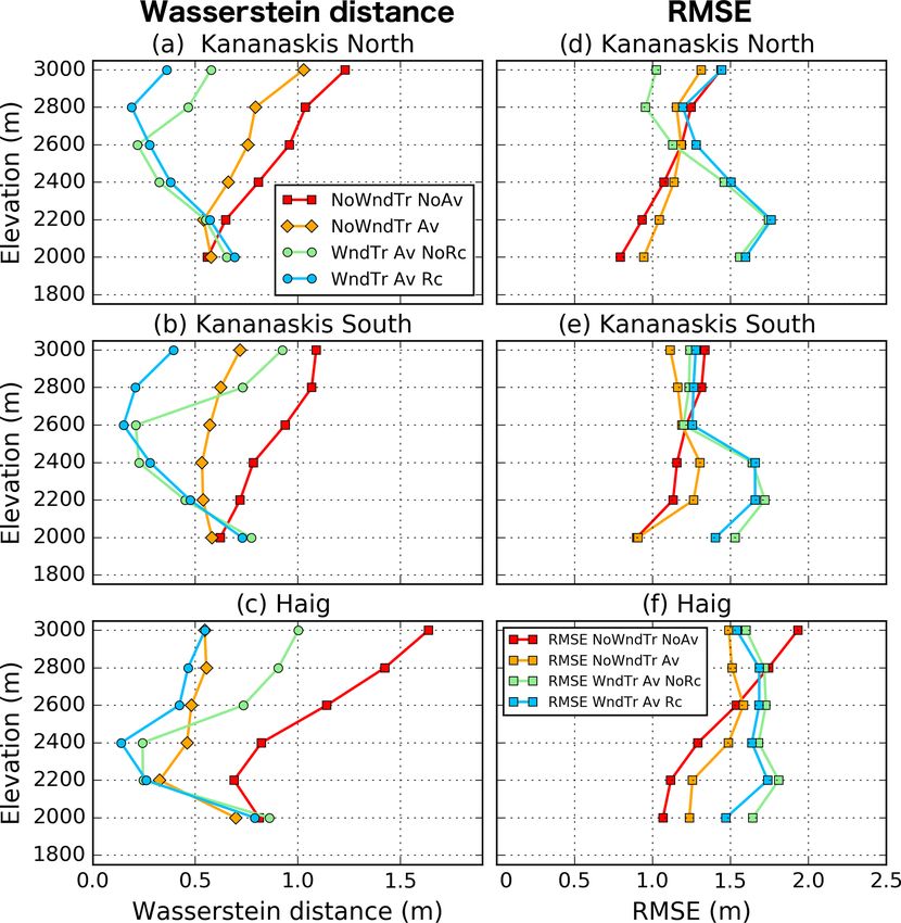
V. Vionnet et al.: Multi-scale snowdrift-permitting modelling of mountain snowpack 751
Table 2. CHM simulations (experiments) used in this study. Rc indicates CHM simulations using wind fields from the downscaling method
accounting for wind speed reduction in leeward areas. HRDPS refers to the High Resolution Deterministic Prediction System and WN to
WindNinja. See text for more details.
Name Driving wind field Gravitational Wind-induced
redistribution snow transport
NoDown HRDPS No No
NoWndTr NoAv HRDPS + WN + Rc No No
NoWndTr Av HRDPS + WN + Rc Yes No
WndTr Av NoRc HRDPS + WN Yes Yes
WndTr Av Rc HRDPS + WN+ Rc Yes Yes
Table 3. Meteorological stations used for wind evaluation. TPI refers to the topographic position index and is defined as the difference
between the elevation of the station minus the mean elevation within a 2 km radius from this station. The location of the stations is shown in
Fig. 1.
Full name Code Latitude Longitude Elevation TPI
(◦ ) (◦ ) (m) (m)
Centennial Ridge CNT 50.9447 −115.9370 2470 248
Fisera Ridge FSR 50.9568 −115.2044 2325 −10
Hay Meadow HMW 50.9441 −115.1389 1492 −33
Fortress Ledge FLG 50.8300 −115.2285 2565 216
Fortress Ridge FRG 50.8364 −115.2209 2327 99
Fortress Ridge South FRS 50.8382 −115.2158 2306 129
Canadian Ridge CRG 50.8215 −115.2063 2211 68
Burtsall Pass BRP 50.7606 −115.3671 2260 −90
compared as a function of slope orientation in the upper et al., 2019). Hansen et al. (2013) global forest product was
slopes using bias and W1 to provide a specific assessment of used to mask out pixels with a tree cover density larger than
model performances in regions particularly exposed to wind- 50 % since the snow retrieval algorithm is not adapted to the
induced snow transport. Upper slopes in the 50 m raster were detection of the snow cover in dense forest areas where the
identified using the TPI as defined above. Regions with TPI ground is obstructed by the canopy. To further avoid misclas-
greater than 150 m were classified as upper slopes. sifications due to forest obstruction or turbid water surfaces,
the DEM was used to mask out pixels below 2000 m. The
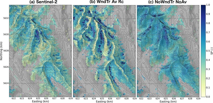
2.3.3 Sentinel-2 snow cover maps final snow product provided the following classification for
each pixel: (i) no snow, (ii) snow, (iii) cloud including cloud
Wayand et al. (2018) suggested that snow persistence in- shadows and (iv) no data.
dices from Sentinel-2 images present a strong potential for Sentinel-2 snow cover maps at 20 m resolution were re-
the evaluation of distributed snow models in mountainous ar- sampled to the same 50 m raster as the CHM output using
eas. Hence, maps of the snow-covered area from the Coper- a median filter. Maps of observed snow persistence (SP) in-
nicus Sentinel-2 satellite mission (Drusch et al., 2012) at dices at 50 m resolution were then derived following Macan-
20 m resolution and at 5 d revisit time were considered as der et al. (2015) and Wayand et al. (2018). SP represents
complementary data to evaluate CHM simulations. Sentinel- for each pixel the ratio between the number of snow-covered
2 images from 1 September 2017 to 31 August 2018 were days and the total number of clear-sky observations (snow or
processed using the snow retrieval algorithm that is cur- no snow). SP was computed using images from 1 April 2018
rently used to produce the Theia Snow collection (Gascoin to 31 August 2018 and SP ranges from 0 (always snow-free)
et al., 2019). First, orthorectified top-of-atmosphere (level to 1 (always snow-covered). Over the study period, the mean
1C) products were processed to bottom-of-atmosphere re- number of clear-sky observations per pixel reached 18.6 d.
flectances (level 2A) using the MAJA software version 3.1 The same calculation was carried out with CHM outputs to
(Hagolle et al., 2017). MAJA output cloud mask and flat- derive maps of simulated snow persistence indices. The same
surface reflectances were used as input to the LIS software dates as the Sentinel-2 maps were used, and for each date, the
version 1.5. The LIS algorithm is based on the normalized Sentinel-2 cloud and no-data masks were applied to make
difference snow index (Dozier, 1989) and uses a digital ele- sure that the same pixels and dates were considered when
vation model to better constrain the snow detection (Gascoin
https://doi.org/10.5194/tc-15-743-2021 The Cryosphere, 15, 743–769, 2021752 V. Vionnet et al.: Multi-scale snowdrift-permitting modelling of mountain snowpack
computing observed and simulated SP indices. A grid cell Figure 4 gives the error metrics for the wind speed (bias
was considered snow-covered if the snow thickness exceeded and RMSE) between the CHM simulations and observations
5 cm (Gascoin et al., 2019). The agreement between the sim- at eight automatic weather stations. The HRDPS without
ulated and the observed SP distributions was quantified as downscaling overestimated wind speed (positive bias) at all
a function of elevation and slope orientation in the upper stations, except the CNT station. This station is located on an
slopes for the same three sub-regions considered for snow exposed crest and presents the largest TPI value among the
depth (i.e., Kananaskis North, Kananaskis South and Haig). stations used for model evaluation (Table 3). Downscaling
Grid cells that were not covered by forest in the observations wind to the CHM mesh using WindNinja microscale winds
and in the simulations were considered for the analysis. (experiment HRDPS + WN) improved the error metrics (de-
crease in bias in absolute value and decrease in RMSE) at
four of the stations (BRP, HMW, FSR and CNT). In partic-
ular, the wind downscaling reduced the negative bias found
3 Results in the HRDPS for the wind-exposed CNT station, presum-
ably because the downscaling captures ridge crest speed-up
The evaluation of the different wind-downscaling methods is of wind velocity. Decreased model performances were found
described in Sect. 3.1. The quality of the snowpack simula- at four neighbouring stations located around the Fortress
tions is then assessed in Sect. 3.2 using airborne lidar snow Mountain Snow Laboratory, however (CRG, FRG, FRS and
depth data and snow persistence indexes. A special emphasis FLG; Fig. 3a). At these stations located along local ridges,
is placed on the ability of the model to capture the elevation– the wind downscaling, accounting for crest speed-up, in-
snow depth relation as well as snow redistribution around creased the wind speed and led to a larger positive bias than
wind-exposed ridges. the default HRDPS (Fig. 3b). Accounting for the formation
of zones of low wind speed in leeward areas in the downscal-
3.1 Wind field downscaling ing method (experiment HRDPS + WN + Rc) was neutral at
two stations located at low elevation (BRP and HMW) and
Figure 3 compares the near-surface wind field obtained from improved results at all remaining stations, except at CNT. In-
a simple bilinear interpolation of the HRDPS wind field deed, a strong degradation of model performance was found
(Fig. 3a) with the downscaled wind field obtained with at this station since it is placed on a sheltered triangle next to
(Fig. 3c) and without (Fig. 3b) the wind speed reduction in the crest on the CHM mesh, leading to an unrealistic reduc-
leeward areas. HRDPS provided a smooth wind field with tion of downscaled wind speed.
relatively higher wind speeds in the northwestern part of the The wind-downscaling method also modified the general
region characterized by high relief (Fig. 3a) compared to the wind direction (Figs. 3 and 5). Prevailing winds during the
rest of the area. HRDPS did not reflect the local terrain infor- study originated from the south (S; 180◦ ) to southwest (SW,
mation due to a horizontal resolution of 2.5 km. Combining 225◦ ) at most of the stations, whereas the HRDPS with-
the HRDPS wind field with precomputed microscale Wind- out downscaling provided wind mainly from the SW–west
Ninja simulations strongly altered the near-surface wind field (W, 270◦ ). Improvements in wind direction when combin-
(Fig. 3b). The downscaled field contained the general pat- ing HRDPS and WindNinja were found for about half of the
tern from the HRDPS modulated by the local-scale terrain meteorological stations. The large error at the CRG station il-
information added by WindNinja and reproduced some typ- lustrated that none of the wind simulation considered in this
ical features of atmospheric flow in complex terrain (e.g., study captured the complex features of the atmospheric flow
Raderschall et al., 2008). In particular, the topography sur- around the Fortress Mountain Snow Laboratory (Fig. 3a).
rounding the main valleys channelled the downscaled atmo-
spheric flow, as illustrated by downscaled wind directions 3.2 Snowpack simulations
aligned parallel to the main valley axes. The presence of
ridge crests generated cross-ridge downscaled flow and as- 3.2.1 Observed and simulated snow distributions
sociated crest wind speed-up. Downscaled wind speeds were
the same on the windward and leeward sides of crests, how- To assess the ability of CHM to simulate small-scale features
ever, as expected with the mass-conserving version of Wind- of snow accumulation and transport in alpine terrain, ALS-
Ninja (Wagenbrenner et al., 2016, 2019). For this reason, an derived snow depths were compared with simulated snow
additional downscaling step using the Winstral parameter to depths for different CHM experiments for a sub-region of
reduce the wind speed in leeward areas was considered as approximately 77 km2 (Fig. 6). Observed snow depth was
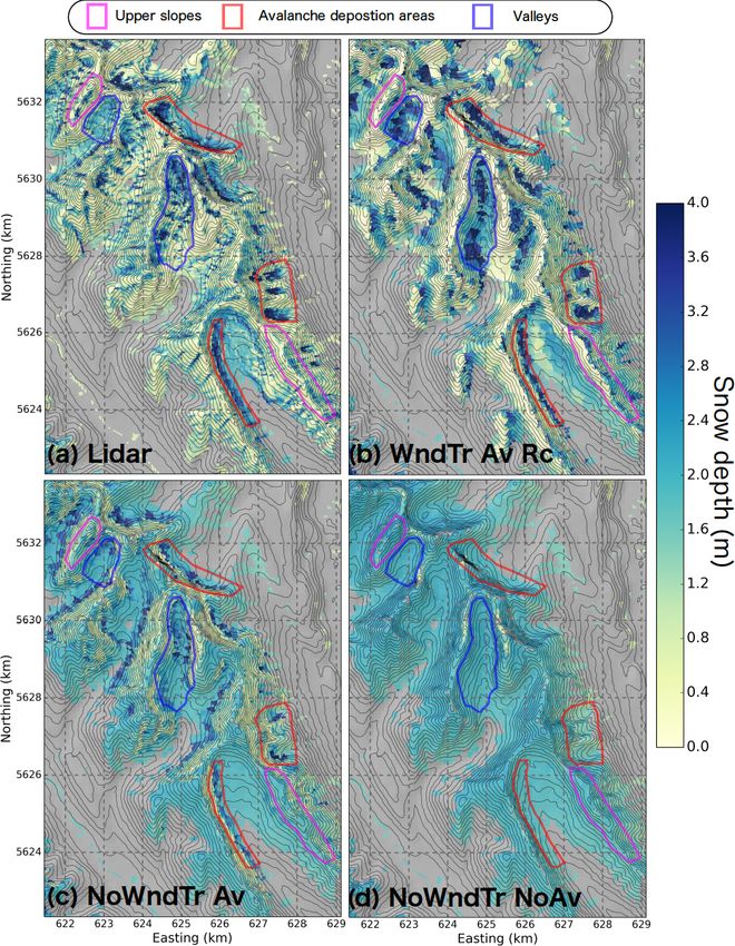
described in Sect. 2.2.4 (Fig. 3c). Blue arrows in Fig. 3c cor- characterized by strong spatial variability (Fig. 6a). Shallow
respond to leeward areas sheltered from the atmospheric flow snow cover (generally less than 1 m) was found in the up-
and characterized by low downscaled wind speed. This addi- per south- to northeast-facing slopes that were primarily ex-
tional downscaling step did not modify the wind direction in posed to wind (Fig. 5). Snow accumulated on the leeward
these areas. side of these slopes (purple contours in Fig. 6a). Thick snow
The Cryosphere, 15, 743–769, 2021 https://doi.org/10.5194/tc-15-743-2021V. Vionnet et al.: Multi-scale snowdrift-permitting modelling of mountain snowpack 753 Figure 3. Near-surface wind field on 10 September 2017 at 18:00 UTC from (a) HRDPS without downscaling, (b) HRDPS downscaled to the CHM mesh M50 15 using WindNinja and (c) same as (b) but including a parameterization for the formation of recirculation zones on leeward slopes (see Sect. 2.2.4 for more details). The location of this sub-area corresponds to the red-shaded area shown in Fig. 1b. Arrows indicate wind direction while colours indicate wind speed. One arrow is shown every 250 m for clarity. The underlying topography is shown using hill shading. Effects of vegetation on the simulated wind fields are not shown in these maps. cover (> 4 m) existed at the bottom of steep slopes and in A better visual agreement with observations was found when large concave cirques corresponding to avalanche deposi- accounting for gravitational snow redistribution in CHM tion areas (red contours in Fig. 6a). The CHM simulation (Fig. 6c). In this configuration, CHM partially reproduced without lateral redistribution of snow (blowing snow and reduced snow accumulation on steep slopes, and avalanche avalanching), NoWndTr NoAv, did not capture these fea- deposits were simulated at the bottom of these slopes (red tures (Fig. 6d). CHM without blowing-snow and avalanche contour in Fig. 6c). However, the model mostly underesti- routines simulated a homogenous snow cover with reduced mated the snow depth in these deposits compared to the ob- snow accumulation for some of the crest regions that are ex- servations (red contours in Fig. 6a) and did not capture the posed to wind and prone to large surface snow sublimation. snow depth distribution in the upper slopes (purple regions https://doi.org/10.5194/tc-15-743-2021 The Cryosphere, 15, 743–769, 2021
754                                       V. Vionnet et al.: Multi-scale snowdrift-permitting modelling of mountain snowpack

                                                                         the region (blue contours in Fig. 6) where avalanche deposi-
                                                                         tion seemed to be overestimated.

                                                                         3.2.2   Elevation dependency of snow depth

                                                                         The agreement between observed and simulated snow depth
                                                                         distributions was examined as a function of elevation for
                                                                         three sub-regions (see Fig. 1) of the Kananaskis domain:
                                                                         Kananaskis North, Kananaskis South and Haig (Figs. 7 and
                                                                         8). For each sub-region, the median of observed snow depth
                                                                         increased with elevation up to 2400 m followed by a decrease
                                                                         at the highest elevations (Fig. 7), a relationship reported else-
                                                                         where (Grünewald et al., 2014; Kirchner et al., 2014). The
                                                                         same trend was found for the other percentiles shown on
Figure 4. Evaluation of simulated wind speed using different down-
                                                                         the whisker plots of the observed distributions of snow depth
scaling methods: (a) bias and (b) root-mean-square error (RMSE).
                                                                         (Fig. 7). All CHM simulations overestimated the snow depth
Grey colours show the HRDPS wind speed without downscaling,
blue colours show the HRDPS wind speed combined with Wind-               below 2100 m for each sub-region, partly explained by the
Ninja microscale winds (HRDPS + WN) and red colours show the             tendency of HRDPS to overestimate precipitation at valley
same configuration as HRDPS+WN including in addition the wind            stations (see stations HMW and UPC in Fig. S1 in the Sup-
speed reduction on leeward slopes. Stations used for evaluation are      plement). The CHM simulation without lateral redistribu-
classified by increasing TPI (Table 3). Their location is shown in       tion of snow (NoWndTr NoAv) did not capture the observed
Fig. 1.                                                                  spatial variability within each elevation band (Fig. 7). In-
                                                                         stead, simulated average snow depth increased with elevation
                                                                         and diverged with observed decreased snow depth recorded
                                                                         with the ALS survey. Therefore, the experiment NoWndTr
                                                                         NoAv presented an increase in the Wasserstein distance and
                                                                         RMSE with elevation (Fig. 8) associated with a continuous
                                                                         decrease in model performance with increasing elevation.
                                                                         Accounting for gravitational redistribution in CHM (exper-
                                                                         iment NoWndTr Av; orange boxes in Fig. 7) increased the
                                                                         spatial variability within each elevation band and reduced
                                                                         snow accumulation above 2400 m, especially for the Haig
                                                                         sub-region (Fig. 7c) characterized by steep slopes prone to
                                                                         avalanching (Fig. 1b). The experiment NoWndTr Av led to
                                                                         improved Wasserstein distance at all elevations for each sub-
                                                                         region compared to the experiment NoWndTr NoAv (Fig. 8).
                                                                         Snow depth above 2300 m for all sub-regions was still over-
Figure 5. Same as Fig. 4 for wind direction: (a) preferential wind di-   estimated, however (Fig. 7). The increase in RMSE below
rection and (b) root-mean-square error (RMSE). Error metrics were        2400 m (Fig. 8) suggested that experiment NoWndTr Av did
computed for wind direction only when observed wind speed was            not capture the location of avalanche deposits well.
larger than 3 m s−1 . Configuration HRDPS+WN+Rc is not shown                Including blowing-snow redistribution strongly affected
since the wind direction is unchanged compared to HRDPS + WN.            model results. As expected, it increased the spatial variability
                                                                         of simulated snow depth within each elevation band com-
                                                                         pared to experiments NoWndTr NoAv and NoWndTr Av
in Fig. 6c). The reference CHM with lateral redistribution of            (Fig. 7). When the wind speed reduction in leeward areas
snow and wind speed reduction in leeward slopes, WndTr                   was not simulated (experiment WndTr Av NoRc), CHM un-
Av Rc, brought large improvements (Fig. 6b). Accounting                  derestimated the median snow depth (as well as the first and
for blowing-snow redistribution reduced snow accumulation                third quartiles) above 2500 m compared to observations. This
on windward slopes and locally increased snow deposition                 underestimation increased with elevation and was largest for
in the upper parts of leeward slopes (purple contours in                 the elevation band 2900–3100 m. Including the recirculation
Fig. 6b). It also led to a large increase in snow accumula-              effect when simulating blowing snow (experiment WndTr Av
tion in avalanche deposition areas (red contours in Fig. 6b)             Rc) strongly improved the ability of the model to capture the
that better corresponded with observed features of snow ac-              distribution of snow depth at high elevation (above 2700 m
cumulation (Fig. 6a). However, WndTr Av Rc presented an                  for Kananaskis North, Fig. 8a; above 2500 m for Kananaskis
overestimation of snow depth in some of the large valleys of             South, Fig. 8b; and above 2100 m for Haig, Fig. 8c). Over-

The Cryosphere, 15, 743–769, 2021                                                             https://doi.org/10.5194/tc-15-743-2021
You can also read