The fractional energy balance equation for climate projections through 2100
←
→
Page content transcription
If your browser does not render page correctly, please read the page content below
Research article
Earth Syst. Dynam., 13, 81–107, 2022
https://doi.org/10.5194/esd-13-81-2022
© Author(s) 2022. This work is distributed under
the Creative Commons Attribution 4.0 License.

                          The fractional energy balance equation
                           for climate projections through 2100
                                  Roman Procyk1 , Shaun Lovejoy1 , and Raphael Hébert2,3
            1 Physics  Department, McGill University, 3600 rue University, Montreal, Quebec, H3A 2T8, Canada
                          2 Alfred-Wegener Institute Helmholtz Centre for Polar and Marine Research,

                                        Telegrafenberg A45, 14473 Potsdam, Germany
          3 Institute of Geosciences, University of Potsdam, Karl-Liebknecht-Str. 24/25, 14476 Potsdam, Germany

                            Correspondence: Roman Procyk (roman.procyk@mail.mcgill.ca) and
                                           Shaun Lovejoy (lovejoy@physics.mcgill.ca)

                                       Received: 2 July 2020 – Discussion started: 4 August 2020
                        Revised: 10 November 2021 – Accepted: 11 November 2021 – Published: 19 January 2022

      Abstract. We produce climate projections through the 21st century using the fractional energy balance equa-
      tion (FEBE): a generalization of the standard energy balance equation (EBE). The FEBE can be derived from
      Budyko–Sellers models or phenomenologically through the application of the scaling symmetry to energy stor-
      age processes, easily implemented by changing the integer order of the storage (derivative) term in the EBE to a
      fractional value.
         The FEBE is defined by three parameters: a fundamental shape parameter, a timescale and an amplitude,
      corresponding to, respectively, the scaling exponent h, the relaxation time τ and the equilibrium climate sensi-
      tivity (ECS). Two additional parameters were needed for the forcing: an aerosol recalibration factor α to account
      for the large aerosol uncertainty and a volcanic intermittency correction exponent ν. A Bayesian framework
      based on historical temperatures and natural and anthropogenic forcing series was used for parameter estima-
      tion. Significantly, the error model was not ad hoc but rather predicted by the model itself: the internal variability
      response to white noise internal forcing.
         The 90 % credible interval (CI) of the exponent and relaxation time were h = [0.33, 0.44] (median = 0.38)
      and τ = [2.4, 7.0] (median = 4.7) years compared to the usual EBE h = 1, and literature values of τ typically
      in the range 2–8 years. Aerosol forcings were too strong, requiring a decrease by an average factor α = [0.2,
      1.0] (median = 0.6); the volcanic intermittency correction exponent was ν = [0.15, 0.41] (median = 0.28) com-
      pared to standard values α = ν = 1. The overpowered aerosols support a revision of the global modern (2005)
      aerosol forcing 90 % CI to a narrower range [−1.0, −0.2] W m−2 . The key parameter ECS in comparison to
      IPCC AR5 (and to the CMIP6 MME), the 90 % CI range is reduced from [1.5, 4.5] K ([2.0, 5.5] K) to [1.6, 2.4] K
      ([1.5, 2.2] K), with median value lowered from 3.0 K (3.7 K) to 2.0 K (1.8 K). Similarly we found for the transient
      climate response (TCR), the 90 % CI range shrinks from [1.0, 2.5] K ([1.2, 2.8] K) to [1.2, 1.8] K ([1.1, 1.6] K)
      and the median estimate decreases from 1.8 K (2.0 K) to 1.5 K (1.4 K). As often seen in other observational-based
      studies, the FEBE values for climate sensitivities are therefore somewhat lower but still consistent with those in
      IPCC AR5 and the CMIP6 MME.
         Using these parameters, we made projections to 2100 using both the Representative Concentration Path-
      way (RCP) and Shared Socioeconomic Pathway (SSP) scenarios, and compared them to the corresponding
      CMIP5 and CMIP6 multi-model ensembles (MMEs). The FEBE historical reconstructions (1880–2020) closely
      follow observations, notably during the 1998–2014 slowdown (“hiatus”). We also reproduce the internal vari-
      ability with the FEBE and statistically validate this against centennial-scale temperature observations. Overall,
      the FEBE projections were 10 %–15 % lower but due to their smaller uncertainties, their 90 % CIs lie completely
      within the GCM 90 % CIs. This agreement means that the FEBE validates the MME, and vice versa.

Published by Copernicus Publications on behalf of the European Geosciences Union.
82                             R. Procyk et al.: The fractional energy balance equation for climate projections through 2100

1    Introduction                                                   els usually involve at least two boxes and they assume New-
                                                                    ton’s law of cooling as well as ad hoc assumptions relating
                                                                    surface temperature gradients to the rate of heat exchange.
The Earth is a complex, heterogenous system with turbu-                Energy conservation is an important symmetry principle,
lent atmospheric and oceanic processes operating over scales        yet when implemented in box-type models, it violates an-
ranging from millimetres up to planetary scales. When con-          other symmetry: scale invariance. This is because box mod-
sidered by timescale, there are three main regimes: the             els are integer ordered differential equations whose response
weather, macroweather and climate (Lovejoy and Schertzer,           functions (Green’s functions) are exponentials (see Ghil and
2013; Lovejoy, 2013). From dissipation times up until the           Lucarini, 2020, for a discussion on the exponential decay of
scale of 10 d (days) – the lifetime of planetary structures –       Green’s function in the climate context). In order to respect
fluctuations in the temperature and other atmospheric quan-         the scaling, these “climate response functions” (CRFs) have
tities increase with timescale: this is the weather regime.         therefore been postulated to be scaling (power law). How-
Beyond this – in macroweather – fluctuations generally              ever, the use of pure power-law CRFs (e.g. Rypdal, 2012;
decrease with scale: averaging anomalies over longer and            Myrvoll-Nilsen et al., 2020) leads to divergences: the “run-
longer times decrease their average. Eventually, this is re-        away Green’s function effect” (Hébert and Lovejoy, 2015)
versed and fluctuations again tend to increase, marking the         which states that if the Earth is perturbed by even an infinites-
beginning of the climate regime. In the industrial epoch,           imal step function forcing, its temperature monotonically in-
this occurs at a scale of ≈ 20 years, while in the pre-             creases without ever attaining thermodynamic equilibrium:
industrial epoch the transition is at centuries or millennia        its equilibrium climate sensitivity (ECS) is infinite. Whereas
and the regime continues up to Milankovitch scales (Love-           the classical EBMs conserve energy but violate scaling, the
joy, 2015b, 2019).                                                  pure scaling CRF models are scaling but violate energy con-
    A major challenge is to determine the Earth’s decadal and       servation. Such models can only make projections by using
centennial response to anthropogenic and natural perturba-          forcings that start and then return to zero.
tions. At the moment, projection uncertainties – famously              Hébert et al. (2021) proposed taming the divergences by
exemplified in the range 1.5–4.5 K for a CO2 doubling –             cutting off the power-law CRFs at small scales. The re-
are so large that for many purposes, including the develop-         sulting model was scaling at long times and, when forced
ment of mitigation policies, the development of complemen-          by step functions, reaches thermodynamic equilibrium. With
tary approaches are needed. When considering alternatives,          this truncated power-law CRF and using Bayesian tech-
although perturbations to the Earth system can be quite var-        niques, Hébert et al. (2021) were able to make climate pro-
ied, when compared to the mean solar radiation, over the past       jections through 2100 with the Intergovernmental Panel on
and future decades, those of interest are of the order of only a    Climate Change (IPCC) Representative Concentration Path-
few percent. This allows diverse forcings to be conveniently        way (RCP) scenario forcings that were coherent with the
approximated by their equivalent radiative forcings. It also        multi-model ensemble (MME) 90 % credible interval (CI).
explains why – in spite of their highly non-linear weather          Furthermore, using the historical part of each GCM simula-
dynamics – that to a good approximation, general circulation        tion, the corresponding GCM climate projections were accu-
model (GCM) macroweather and climate responses to deter-            rately reproduced, meaning (in regards to the Earth’s glob-
ministic external perturbations are typically linear (as quan-      ally averaged temperature) that both models were effectively
tified for CMIP5 models in Hébert and Lovejoy, 2018) but            equivalent. The caveat was that the CRF model truncation
with stochastic internal variability.                               was somewhat ad hoc and therefore only useful at decadal or
    In order to construct macroweather and climate mod-             longer scales.
els, beyond linearity and stochasticity, we require additional         To make more realistic models, the key issue is energy
model constraints, the classical one being energy balance.          storage. Storage is a consequence of imbalances in incom-
Starting with the first energy balance models (EBMs) pro-           ing short wave and outgoing long wave radiation and it must
posed by Budyko (1969) and Sellers (1969), EBMs and                 be accounted for in applications of the energy balance prin-
stochastic climate models have been extensively used for            ciple (Trenberth et al., 2009). As pointed out in Lovejoy
understanding the climate (North, 1975; Hasselmann, 1976;           (2019, 2022) and developed in Lovejoy et al. (2021), it is
North et al., 1981; Imkeller and Von Storch, 2001; Trenberth        sufficient that the scaling principle not be applied to the CRF
et al., 2014; North and Kim, 2017; Proistosescu et al., 2018;       but rather to the storage term in the EBE. In lieu of the en-
Ziegler and Rehfeld, 2021). In this paper, we will only con-        ergy being stored by uniformly heating a box, energy is in-
sider EBMs for the globally averaged temperature. The re-           stead stored in a hierarchy of structures from small to large,
sulting “zero-dimensional” energy balance equation (EBE) is         each with time constants that are power laws of their sizes.
a first-order linear differential equation; it can be obtained by   This conceptual shift can be implemented simply by chang-
considering the Earth to be a uniform slab of material (“box”)      ing the integer order of the storage (derivative) term in the
radiatively exchanging heat with outer space. Such box mod-

Earth Syst. Dynam., 13, 81–107, 2022                                                    https://doi.org/10.5194/esd-13-81-2022
R. Procyk et al.: The fractional energy balance equation for climate projections through 2100                                              83

EBE to a fractional value: the fractional energy balance equa-     (Lovejoy, 2022; Lovejoy et al., 2021), where T (t) is the Earth
tion (FEBE). While Lovejoy et al. (2021) derived the FEBE          temperature anomaly with respect to a reference temperature
in a phenomenological manner, Lovejoy (2021a, b) showed            (limt→−∞ T (t) = 0), τ is the relaxation time, s is the climate
how it could instead be derived from the classical continuum       sensitivity, F(t) is the anomalous external radiative forcing
mechanics heat equation used in the Budyko–Sellers models.         which is the sum of stochastic f (t) and deterministic F (t)
Indeed, by extending Budyko–Sellers models from 2-D to 3-          components, and h is the order of the Weyl fractional deriva-
D (i.e. to include the vertical) and imposing the (correct) con-   tive (see, e.g. Podlubny, 1999):
ductive – radiative surface boundary conditions, one immedi-
ately obtains fractional-order equations for the surface tem-                                 Zt
                                                                       h            1                                               dT
perature. In other words, nonclassical fractional equations        −∞ Dt T     =                   (t − u)−h T 0 (u)du, T 0 (u) =      ,   (2)
                                                                                 0(1 − h)                                           du
and long memories turn out to be necessary consequences                                      −∞
of the classical Budyko–Sellers approach.
                                                                   where 0 is the gamma function. If this derivative is integrated
   To understand the FEBE’s key new features, recall that lin-
                                                                   by parts and the limit h → 1 is taken, using limt→−∞ T (t) =
ear differential equations can be solved with Green’s func-
                                                                   0, −∞ Dth T = dTdt so that we recover the standard box EBE
tions; in the classical integer-ordered case, these are based
                                                                   (Lovejoy et al., 2021).
on exponentials. However, in the general case where one or
                                                                      If we solve the FEBE using Green’s functions, we obtain
more terms are of fractional order, they are instead based
on “generalized exponentials”, themselves based on power                       Zt
laws. In the FEBE, there are two distinct power-law regimes        T (t) = s         G0,h (t − u)F(u)du,                                   (3)
with a transition at the relaxation time (estimated to be of the
                                                                             −∞
order of a few years; see below). While the low-frequency
Green’s function can be very close to Hébert et al. (2021)’s       where G0,h is the impulse (Dirac) response Green’s function.
truncated power-law CRF, the high-frequency regime is able         For the FEBE, it is given by
to produce internal variability coherent with the observed                    (         h−1          h
scaling and fractional Gaussian noise used for skilfully fore-                  τ −1 τt      Eh,h − τt      ; t ≥0
                                                                   G0,h (t) =                                               (4)
casting the stochastic (internal) variability at monthly, sea-                  0;                            t < 0,
sonal and interannual (macroweather) scales (Lovejoy et al.,
2015; Del Rio Amador and Lovejoy, 2019, 2021a). In short,          where
there are theoretical arguments as well as empirical evi-                       ∞
                                                                                X           zk
dence that the FEBE accurately models the Earth’s tem-             Eα,β (z) =                                                              (5)
perature response to both internal and external forcing over                        k
                                                                                         0(αk + β)
macroweather and climate timescales.
   The following text introduces the FEBE (Sect. 2.1), de-         is the “α, β-order Mittag–Leffler function” (these and most
scribes the radiative forcing, temperature and GCM simu-           of the following results are in the notation of Podlubny,
lations that are used (Sect. 2.2), and introduces Bayesian         1999). The condition G0,h (t) = 0 for t < 0 is needed to re-
inference for determining the model and forcing parame-            spect causality; in what follows, this is implicitly assumed for
ters (Sect. 2.3). Using these, we present the probability dis-     all Green’s functions. The Mittag–Leffler functions are of-
tribution functions for the parameters (Sect. 3.1 and 3.2)         ten called “generalized exponentials”; the classical h = 1 box
and estimate the ECS and transient climate response (TCR)          model is the (exceptional) ordinary exponential: E1,1 (z) =
(Sect. 3.3). Using our parameters, we discuss the model reli-      ez .
ability and statistically analyse the FEBE (Sect. 4), produce          Mathematically, when 0 < h < 1, the FEBE is a “frac-
global projections to 2100 using the RCPs and Shared So-           tional relaxation equation” where τ quantifies the slow,
cioeconomic Pathways (SSPs), and estimate the probabil-            power-law approach to a new thermodynamic equilibrium.
ity of exceeding various warming thresholds all of which           Rather than express solutions in terms of the impulse re-
we compare to the corresponding CMIP5 and CMIP6 GCM                sponse G0,h , it is often more convenient to use the step re-
MMEs (readers only wanting results can skip to Sect. 5).           sponse G1,h :

                                                                                Zt                    h           h !
                                                                                                      t             t
                                                                   G1,h (t) =           G0,h (u)du =      Eh,h+1 −        ,                (6)
2     Methods and material                                                                            τ             τ
                                                                                0

2.1    The FEBE                                                    such that the temperature response can be written as
The zero-dimensional FEBE may be written as                                    Zt
                                                                                                                         dF
                                                                   T (t) = s         G1,h (t − u)F 0 (u)du, F 0 (u) =       .              (7)
 h
τ−∞ Dth T   + T = sF, F(t) = F (t) + f (t), 0 ≤ h ≤ 1       (1)                                                          du
                                                                             −∞

https://doi.org/10.5194/esd-13-81-2022                                                       Earth Syst. Dynam., 13, 81–107, 2022
84                            R. Procyk et al.: The fractional energy balance equation for climate projections through 2100

G1,h has the advantage of being dimensionless, and it also
has a simple interpretation as being the response to a step                                     ρ
                                                                   FCO2 (ρ) = 3.71 W m−2 log                                  (10)
forcing such as that found in numerical CO2 doubling exper-                                     ρ0
iments. At high frequencies (t  τ ), important for modelling
                                                                   where FCO2 is the forcing due to carbon dioxide, ρ is the con-
and predicting the internal variability, we have
                                                                   centration of carbon dioxide, and ρ0 is the pre-industrial con-
                   1
                        h−1
                        t                                          centration of carbon dioxide, which we take to be 277 ppm
G0,h,high (t) =                ,                                   (Solomon, 2007).
                τ 0(h) τ
                          h                                         We follow the CMIP5 recommendations for anthro-
                     1     t                                       pogenic and solar forcing, while volcanic forcing is unpre-
G1,h,high (t) =                ; t  τ.                   (8)
                0(h + 1) τ                                         scribed (Taylor et al., 2012). The anthropogenic CMIP6 ra-
                                                                   diative forcings follow C. J. Smith et al. (2018).
These correspond to taking the first terms in the series ex-
pansions for the Mittag–Leffler functions in Eqs. (4) and (6).
                                                                   2.2.2   Greenhouse gas forcing
If we consider the response to Gaussian white noise forc-
ing, γ (t), then G0,h (t) ∝ t h−1 implies that T (t) is approxi-   The global climate is warming and most of the observed
mately a fractional Gaussian noise (fGn) with statistical scal-    changes are due to increases in the concentration of anthro-
ing exponent h − 1/2 (when forced by a Gaussian white              pogenic greenhouse gases (GHGs) (IPCC, 2013). Future an-
noise, the FEBE response is exactly a fractional Relaxation        thropogenic forcing is prescribed in the Representative Con-
noise, see Lovejoy, 2022). In Lovejoy et al. (2015); Lovejoy       centration Pathways (RCPs), established by the IPCC for
(2015a), the high-frequency approximation with an exponent         CMIP5 simulations: we considered RCP2.6, RCP4.5 and
corresponding to h = 0.3 was used; in Del Rio Amador and           RCP8.5 (Meinshausen et al., 2011b). RCP6.0 was omitted in
Lovejoy (2019), forecasts with the more accurate estimate          this study since fewer CMIP5 modelling groups performed
h ≈ 0.4 ± 0.05 (see below) were used.                              the associated run. In the CMIP6 simulations, the anthro-
   To see if this is compatible with the value estimated from      pogenic forcings are prescribed in the Shared Socioeconomic
the low-frequency response to external forcings, consider the      Pathways (SSPs) (Meinshausen et al., 2020); we investigate
low-frequency behaviour (t  τ ) important for modelling           the SSP1-26 (strong mitigation), SSP2-45 (middle of the
and projecting the multidecadal responses to external forc-        road) and SSP5-85 (strong emission) scenarios, designated
ing:                                                               as high priority for IPCC AR6 and counterparts to the previ-
                          −1−h                                   ous RCP scenarios above.
                   −1      t                                          The RCP scenarios are derived from estimates of emis-
G0,h,low (t) =                     ,
                τ 0(−h) τ                                          sions computed by a set of integrated assessment mod-
                        1
                               −h
                                t                                  els (IAMs); these emissions are converted to concentra-
G1,h,low (t) = 1 −                   ; t τ                  (9)   tions using the Model for the Assessment of Greenhouse-
                    0(1 − h) τ
                                                                   gas Induced Climate Change (MAGICC, Meinshausen et al.,
(note 0(−h) < 0 for 0 < h < 1). In the box model case,             2011a), while for the SSP scenarios the emissions are con-
h = 1, we have exactly G1,1 (t) = 1 − e−t/τ , whereas when         verted to forcings using the Finite Amplitude Impulse Re-
h < 1, the exponential approach to equilibrium is replaced by      sponse model (FAIR, C. J. Smith et al., 2018). These scenar-
                                                            H
a power law. Hébert et al. (2021) used G1 (t) = 1− 1 + τt F        ios will allow us to compare our results from the FEBE with
with HF ≈ −0.5−0.5+0.4
                       corresponding for t  τ to h = −HF ≈        CMIP5/6 simulations.
0.5, which is thus (within the uncertainty) the same h value as       The wide spread between the scenarios allows for the in-
that corresponding to the internal forcing. It is thus plausible   vestigation of the consequences of various future policies,
that the FEBE models both high- and low-frequency regimes          from strong mitigation (RCP2.6, SSP1-26) to no-policy ref-
with the unique exponent h ≈ 0.4. Indeed, it was this empir-       erence (RCP8.5, SSP5-85) shown in Fig. 1a. For RCP2.6 and
ical finding that predated and motivated the discovery of the      SSP1-26, the strongest mitigation scenarios, the total radia-
FEBE.                                                              tive forcing has a peak at approximately 3 W m−2 around the
                                                                   year 2050 and declines thereafter due to large-scale deploy-
                                                                   ment of negative emission technologies. RCP4.5 and SSP2-
2.2     Data
                                                                   45 are stabilization scenarios, with the total radiative forcing
2.2.1    Radiative forcing data                                    rising until the year 2070 and with stable concentrations after
                                                                   the year 2070. In contrast, RCP8.5 and SSP5-85 are contin-
We consider natural and anthropogenic sources of ex-               uously rising radiative forcing pathways in which the radia-
ternal forcing: solar and volcanic, greenhouse gases and           tive forcing levels by the end of the 21st century reach ap-
aerosols. We use the standard semi-empirical carbon-               proximately 8.5 W m−2 . Current emissions fall somewhere
dioxide-concentration-to-forcing relationship (Myhre et al.,       between the 4.5 and 8.5 W m−2 scenarios.
1998):

Earth Syst. Dynam., 13, 81–107, 2022                                                   https://doi.org/10.5194/esd-13-81-2022
R. Procyk et al.: The fractional energy balance equation for climate projections through 2100                                    85

                                                                        We obtained the CMIP5 aerosol forcing from the to-
                                                                     tal CO2eq forcing by subtracting the combined effective ra-
                                                                     diative forcing of the gases controlled by the Kyoto proto-
                                                                     col, FKyt , and from those controlled under the Montreal pro-
                                                                     tocol, FMtl . FMtl is given in CFC-12 equivalent concentration
                                                                     and we use the relation from Ramaswamy et al. (2001) to
                                                                     convert this to W m−2 .
                                                                        The total amount of aerosol forcing in 2005 given at
                                                                     the 90 % CI in the IPCC Fifth Assessment Report (AR5) is
                                                                     [−1.9, −0.1] W m−2 . However, since then, attempts have
                                                                     been made to better constrain this value; Stevens (2015)
                                                                     argues that extreme aerosol forcings (more negative than
                                                                     −1 W m−2 ) are implausible. Using results from Murphy
                                                                     et al. (2009), Stevens (2015) supports tightening the up-
                                                                     per and lower bounds of the aerosol forcing, revising it to
                                                                     [−1.0, −0.3] W m−2 , although the wider range from the
                                                                     IPCC’s AR5 is still supported by the more comprehensive
                                                                     study by Bellouin et al. (2020).
                                                                        The prescribed CMIP6 SSP aerosol forcing, FAerSSP , con-
                                                                     tains contributions from aerosol–radiation interactions and
Figure 1. (a) The anthropogenic forcing series, the sum of the
                                                                     from aerosol–cloud interactions: Fari and Faci (C. J. Smith
greenhouse gas forcing FGHG and respective aerosol forcing se-       et al., 2018). Fari includes the direct radiative effect of
ries FAerRCP (black) or FAerSSP (blue) are shown over the histor-    aerosols, in addition to rapid adjustments due to changes in
ical period and projection period until 2100 for RCP2.6/SSP1-26      the atmospheric temperature, humidity and cloud profile (for-
(solid), RCP4.5/SSP2-45 (dashed) and RCP8.5/SSP5-85 (dotted).        merly the “semi-direct effect”), and is calculated using multi-
(b) The anthropogenic aerosol forcing series used, FAerRCP (blue)    model results from AeroCom (Myhre et al., 2013). Faci de-
and FAerSSP (black), following the same scheme as above. Updated     scribes how aerosols affect clouds in the radiation budget
from Hébert et al. (2021).                                           and is calculated from the aerosol model of Stevens (2015),
                                                                     which includes a logarithmic dependence of Faci on sul-
                                                                     fates, black carbon and organic carbon emissions – the source
   In this paper, we use the forcing due to carbon dioxide           of the difference in aerosol forcing shapes between FAerRCP
equivalent, FCO2eq , as the measure of our anthropogenic forc-       and FAerSSP shown in Fig. 1b.
ing, FAnt , given in the RCP and SSP scenarios. The anthro-
pogenic forcing from gases corresponds to the effective ra-
diative forcing produced by long-lived GHGs FGHG : carbon            2.2.4   Solar forcing
dioxide, methane, nitrous oxide and fluorinated gases, con-          The other external forcings considered are solar and volcanic.
trolled under the Kyoto Protocol, and ozone-depleting sub-           Although there exist other natural forcings such as mineral
stances, controlled under the Montreal Protocol. We show             dust and sea salt, they are small and will be implicitly in-
the anthropogenic forcings for each RCP and SSP scenario             cluded with the internal variability. We use the CMIP5 rec-
in Fig. 1.                                                           ommendation for solar forcing, FSol , a reconstruction ob-
                                                                     tained by regressing sunspot and faculae time series with
2.2.3   Aerosol forcing                                              total solar irradiance (TSI) (Wang et al., 2005), shown in
                                                                     Fig. 2. Following Meinshausen et al. (2011b), the solar forc-
Aerosols are a strong component of radiative forcing associ-         ing anomaly is calculated as the change in solar constant over
ated with anthropogenic emissions, resulting from a combi-           the average value of the two 11-year solar cycles from 1882
nation of direct and indirect aerosol effects. There exists high     to 1904 divided by 4 (the effective fraction of the surface of
uncertainty of the aerosol forcing, arising from a poor un-          the Earth which is exposed to the Sun) and multiplied by 0.7
derstanding of how clouds respond to aerosol perturbations           (representing planetary co-albedo). To extend solar forcing
(Penner et al., 2001; Ramaswamy et al., 2001), compared to           to the future, we follow CMIP5 and reproduce solar cycle 23
the fairly well-constrained GHG forcing. We therefore fol-           (the last one prior to 2008) as the assumed future solar forc-
low Forest et al. (2002), Harvey and Kaufmann (2002), For-           ing.
est et al. (2006), Padilla et al. (2011) and Hébert et al. (2021);
we introduce the aerosol linear scaling factor α to account for
our poor knowledge of aerosol forcing.

https://doi.org/10.5194/esd-13-81-2022                                                   Earth Syst. Dynam., 13, 81–107, 2022
86                              R. Procyk et al.: The fractional energy balance equation for climate projections through 2100

                                                                         The normalization is such that the mean is unchanged:
                                                                      hFVolν i = hFVol i; the average volcanic forcing is conserved
                                                                      – this was done for simplicity and if needed future work
                                                                      could include another scaling parameter (this is slightly dif-
                                                                      ferent than the normalization used in Hébert et al., 2021).
                                                                      The volcanic intermittency correction exponent, ν, required
                                                                      to reduce the intermittency parameter of the volcanic forc-
                                                                      ing, C1,FV , to equal the corresponding parameter of the tem-
                                                                      perature response, C1,TV , can be calculated theoretically us-
                                                                      ing:

                                                                      C1,FV ν αMF = C1,TV ,                                        (12)
Figure 2. Volcanic forcing FVol1 (blue) is shown alongside two
transformed versions: linearly damped by a constant 0.5 coefficient   where αMF is the multifractality index of the volcanic forc-
(black) and non-linearly transformed using Eq. (11) with ν = 0.3      ing and C1 is the codimension of the mean (see Chapter 4,
(red). The solar forcing FSol (orange) has been shifted down by −9    Lovejoy and Schertzer, 2013).
and amplified by a factor of 10 for clarity. The figure has been         The volcanic response appears to be non-linear as the in-
adapted from Hébert et al. (2021).                                    termittency (“spikiness”, sparseness of the spikes) parame-
                                                                      ter C1 changes from about C1,FV ≈ 0.16 for the input vol-
2.2.5   Volcanic forcing                                              canic forcing to C1,T ≈ 0.03 for the temperature response:
                                                                      the latter is therefore much less intermittent than the for-
The volcanic forcing series, FVol , used in this study was            mer, although it is possible that the estimated C1 changes
generated from the volcanic optical depths, τV . Over the             slightly due to finite size effects and internal variability. As-
1850 to 2012 period, we use the approximate relation:                 suming αMF ≈ 1.5 (Lovejoy and Schertzer, 2013; Lovejoy
FVol ≈ −27 W m−2 τV , obtained from the Goddard Institute             and Varotsos, 2016), we find an approximate but plausible
for Space Science (GISS) website (Sato et al., 1993). We fol-         theoretical estimate of the volcanic intermittency correction
low Hébert et al. (2021), extending the series to 1765 using          exponent ν ≈ 0.3.
the optical depth reconstruction of Crowley et al. (2008) and
setting volcanic forcing to zero for the future.                      2.2.6   Internal stochastic forcing
   It is well established that volcanic forcing must be scaled
down by 40 %–50 % in order to produce a comparable effect             We consider the standard assumption about internal variabil-
on surface temperature, and thus most EBMs linearly scale             ity that it is forced by a Gaussian “delta-correlated” white
volcanic forcing (Tomassini et al., 2007; Ring et al., 2012;          noise (Hasselmann, 1976):
Lewis and Curry, 2015; Gregory and Andrews, 2016). How-
ever, the amplitude of the volcanic forcing is not the only           f (t) = σ γ (t); hγ (t)i = 0; hγ (t)γ (u)i = δ(t − u),       (13)
issue; volcanic forcings are highly intermittent (spiky). The         where f (t) is the noise at infinite resolution, γ (t) is a “unit”
intermittency can be quantified in a multifractal framework           white noise and σ is its amplitude. When averaged to res-
(Lovejoy and Schertzer, 2013; Lovejoy and Varotsos, 2016)             olution τr = 1 month, the average forcing has amplitude
by the intermittency parameter C1 which corresponds to the            hfτ2r i1/2 = στ = √στr . In comparison, the internal variability
fractal codimension (i.e. 1-D, where D is the fractal dimen-
                                                                      of the mean observational temperature series is equal to the
sion of the part of series that gives the dominant contribution
                                                                      observed series with the forced temperature response re-
to the mean of the series) characterizing the sparseness of
                                                                      moved. We take the global annually averaged monthly tem-
volcanic “spikes” of mean amplitude. There is also a mul-
                                                                      perature anomaly to be σT ,τr ≈ ±0.14 ◦ C, where τr is the res-
tifractal index αMF that describes how quickly the intermit-
                                                                      olution (taken to be monthly in this case).
tency changes as we move away from the mean. Since linear
                                                                         Using Lovejoy et al. (2021) and Lovejoy (2022) and σT ,τr ,
response models do not alter the intermittency, the volcanic
                                                                      we can relate σT ,τr and σf,τr :
series must first be non-linearly transformed before being in-
troduced into a linear response framework. With the effective
                                                                              σT ,τr Kh τ h

volcanic forcing FVolν , the volcanic intermittency correction        σf,τr =               ,                                      (14)
exponent ν and the mean of the whole volcanic series hFVol i,                     s      τr
                                                                             v
we follow Hébert et al. (2021) using a non-linear relation to                u              π
                                                                      Kh = u                             ,                         (15)
change the intermittency so that the transformed signal can                  t
                                                                               2 cos π h − 12 0(−1 − 2h)
be linearly related to the temperature:
FVolν    Fν                                                           where Kh is a standard normalization constant, τ is the relax-
       = Vol
          ν i.                                                (11)
hFVol i hFVol                                                         ation time, and s is the climate sensitivity parameter; Eq. (14)

Earth Syst. Dynam., 13, 81–107, 2022                                                       https://doi.org/10.5194/esd-13-81-2022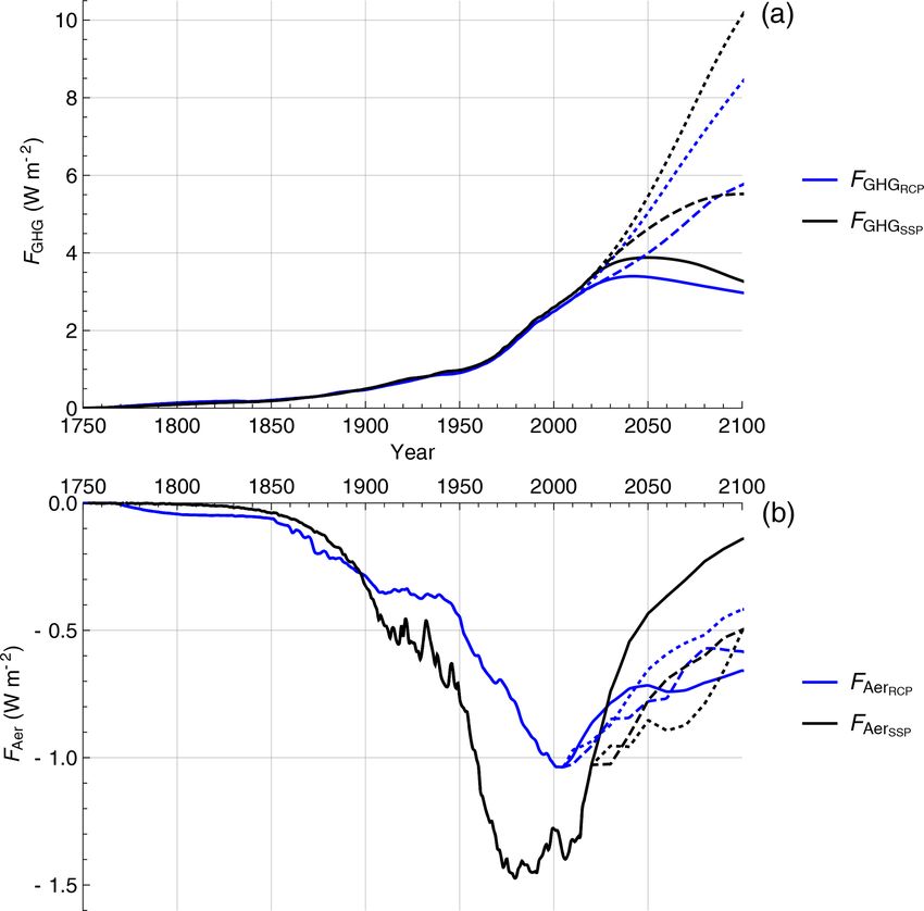
R. Procyk et al.: The fractional energy balance equation for climate projections through 2100                                        87

is an approximation to the FEBE response to white noise              The selected CMIP5 models have monthly historical sim-
forcing valid at short timescales τr  τ . If we introduce a      ulation outputs available over the 1860 to 2005 period
white noise forcing, with the standard deviation calculated       along with outputs of scenario runs from 2005 to 2100 for
using Eq. (14), the FEBE response will correspond to an in-       RCP2.6, RCP4.5 and RCP8.5, summarized in Table A1. The
ternal variability term with realistic amplitude and autocor-     CMIP6 model outputs have monthly historical simulations
relation structure.                                               from 1860 to 2014 and future projections based on the SSP
   Working in a linear framework, we write the forcing se-        scenarios 1-26, 2-45 and 5-85 (Forster et al., 2020) and the
ries, F, as the sum of the deterministic forcings, F , (GHG,      climate sensitivity of models are summarized in Table A2
aerosol, solar and volcanic) and the white noise forcing:         (Flynn and Mauritsen, 2020).

F(α, ν; t) = FGHG (t) + αFAer (t) + FSol (t) + FVolν (t)
                                                                  2.3   Bayesian parameter estimation
          + σf,τr γτr (t);
                                                                  In this section, we establish a procedure to estimate the prob-
F (t) = hF(t)i = FGHG (t) + αFAer (t) + FSol (t)                  ability distribution associated with the climate sensitivity: s,
                                                                  model parameters: τ , h and forcing parameters: α, ν. To es-
     + FVolν (t),                                          (16)   timate them, we relate the forcing to surface air temperature
                                                                  data using the FEBE with a multi-parameter Bayesian tech-
where γτr (t) is a unit of white noise at resolution τr and
                                                                  nique. To apply Bayesian inference, we require temperature
“h i” is the mean ensemble (statistical) average.
                                                                  observations, a statistical model that relates forcing data to
                                                                  temperature and prior information about the model parame-
2.2.7   Surface air temperature data and CMIP5/6                  ters (priors). Bayesian inference is chosen due to its ability to
        simulations                                               better constrain model parameters by using information from
We used five historical records of surface air temperature for    different sources including data and models.
our analysis each spanning the period 1880–2020, with me-            Through this framework, each parameter combination (h,
dian monthly temperature anomalies in relation to the refer-      τ for G0,h and α, ν for F as well as s) produces a time-
ence period of 1880–1910: Hadley Centre/Climatic Research         dependent forced response which is associated with a likeli-
Unit Temperature version 4 (HadCrut4, Morice et al., 2012),       hood that depends on how well the corresponding model out-
the Cowtan and Way reconstruction version 2.0 (C&W, Cow-          put matches the observational temperature records over the
tan and Way, 2014a, b; Cowtan et al., 2015), GISS Sur-            historic period. To see how this works, recall that the FEBE
face Temperature Analysis (GISTEMP, Lenssen et al., 2019),        describes the temperature response to the sum of the exter-
NOAA Merged Land Ocean Global Surface Temperature                 nal deterministic forcing F (t) and an amplitude σ internal
Analysis Dataset (NOAAGlobalTemp, Zhang et al., 2019;             stochastic forcing σ γ (t):
Huang et al., 2020) and Berkeley Earth Surface Temperature
                                                                                                 Text (t) = sG0,h (t) ∗ F (t)
(BEST, Rohde and Hausfather, 2020).                               T (t) = Text (t) + Tint (t);                                  ,   (17)
                                                                                                 Tint (t) = sG0,h (t) ∗ σ γ (t)
   The HadCRUT4 dataset is a combination of the sea-
surface temperature records: HadSST3 was compiled by the          where Text , Tint indicates the responses, and ∗ indicates con-
Hadley Centre of the UK Met Office along with land surface        volution (Eq. 3). Any given set of parameters defines a forced
station records: CRUTEM4 from the Climate Research Unit           temperature response Text (t), and when removed from the ob-
in East Anglia; the Cowtan and Way dataset uses HadCRUT4          servation temperature series, they define a series of residuals:
as raw data but interpolates missing data that would lead to
bias especially at high latitudes by infilling missing data us-   Tres (t) = T (t) − Text (t) = Tint (t) = sG0,h (t) ∗ σ γ (t).     (18)
ing an optimal interpolation algorithm (kriging); we use the
dataset with land air temperature anomalies interpolated over        The residuals are thus equal to the internal temperature
sea ice. The GISTEMP dataset combines the Global Histori-         variability, i.e. the response to the internal forcing σ γ (t).
cal Climate Network version 3 (GHCNv3) land surface air           Here, we make the usual assumption that γ (t) is a Gaus-
temperature records with the Extended Reconstructed Sea           sian white noise so that Tres (t) = Tint (t) is a fractional re-
Surface Temperature version 4 (ERSST) along with the tem-         laxation noise process (fRn, Lovejoy, 2022). However, for
perature dataset from the Scientific Community on Antarctic       scales shorter than the relaxation time τ (of the order of
Research (SCAR) and is compiled by the Goddard Institute          years), the fRn process is very close to a fGn process (due to
for Space Studies; the NOAA National Climate Data Center          the approximation G0,h ≈ G0,high,h , Eq. 8). Thus, rather than
uses GHCNv3 and ERSST but applies different quality con-          making an ad hoc assumption about the statistics of the resid-
trols and bias adjustments. The final dataset, BEST, makes        uals, in our approach the statistics are given by the model
use of its own land surface air temperature product along         itself (a key improvement from Hébert et al., 2021). The
with a modified version of HadSST.                                fGn approximation takes into account the strong power-law
                                                                  correlations induced by the fractional derivative term in the

https://doi.org/10.5194/esd-13-81-2022                                                   Earth Syst. Dynam., 13, 81–107, 2022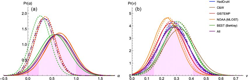
88                                  R. Procyk et al.: The fractional energy balance equation for climate projections through 2100

FEBE and it is generally valid except at the low frequencies                  modern value of aerosol forcing, FAer ≈ −1.0 W m−2 , in the
that only weakly influence the likelihood function. An fGn                    series we used. For the remaining two parameters, s and ν,
model for the residuals is more realistic with respect to the                 we assume non-informative uniform priors over the range of
autocorrelation function of temperature data (Lovejoy et al.,                 parameters; s ∈ [1.0, 4.0] and ν ∈ [0.0, 1.0]. All prior distri-
2015) and thus produces more conservative credible inter-                     butions are independent.
vals in comparison to other exponential decorrelation models                     Using Bayes, Eq. (20), we then fit a multivariate Gaussian
such as an AR(1) since the latter underestimate the decorre-                  distribution to our five-dimensional parameter space, poste-
lation time and thus overestimate the effective sample size.                  rior distribution Pr(s, h, τ, α, ν|T (t)), which will be used to
   To calibrate the FEBE, we take the time-dependent forced                   draw sets of parameters to generate future forced temperature
response calculated for each parameter combination and re-                    projections. The multivariate Gaussian approximation is built
move it from the temperature series to obtain a series of resid-              by using the means and variances of all parameters through
uals which represent an estimator of the historical internal                  integrating the joint probability to obtain five marginal prob-
variability. The likelihood function (L) corresponds to the                   abilities and calculating the covariance between all pairwise
probability (“Pr”) of observing the series T (t) conditioned                  parameters using their “joint” marginal distributions as to
on the parameters: s, h, τ , α, ν (right-hand side), assuming                 take into account potentially large correlations between pa-
the residuals are a fGn process with parameter h, and zero                    rameters. The five-dimensional posterior parameter space, (s,
mean:                                                                         h, τ , α, ν) is thus defined by a multivariate normal distribu-
                                                                              tion:
L(s, h, τ, α, ν|T (t)) = Pr(T (t)|s, h, τ, α, ν).                    (19)
                                                                                                   1                 T 6 −1 (x−µ)/2
                                                                              P (x; µ, 6) =                1
                                                                                                               e−(x−µ)                ,     (21)
   Using Bayes’ rule, we can obtain the posterior probability                                        5
                                                                                                     2 |6|
                                                                                                           2
                                                                                              (2π)
density function (PDF) for our parameters using the likeli-
hood function (an a priori probability) and the prior distribu-               where x = {s, τ, h, α, ν}, the vector of the means is µ and the
tion for the parameters, π (s, h, τ, α, ν):                                   5 × 5 covariance matrix 6.
                            Pr(T (t)|s, h, τ, α, ν)π (s, h, τ, α, ν)
Pr(s, h, τ, α, ν|T (t)) =                                            . (20)   3   Results
                                           Pr(T (t))

   We use the following Mathematica 12.2 (Wolfram Re-                         Using Bayes’ theorem as described above, we derive PDFs
search, Inc., 2020) functions: LogLikelihood[proc, data],                     for the model and forcing parameters of the FEBE from the
FractionalGaussianNoiseProcess[µ, σ 0 , h0 ] and Estimated-                   mean likelihood functions of the five observational datasets.
Process[data, proc] to calculate the maximum likelihood of                    The different observational datasets are treated as dependent
those residuals to be a fGn corresponding to our error model.                 due to the use of overlapping raw data, with the differences
Note that the Hurst exponent h0 used within Mathemat-                         between series coming partly from the different processing of
ica 12.2 describes the scaling behaviour of the associated                    the raw data by different teams. This corresponds to putting
fractional Brownian motion obtained by integrating the fGn                    the datasets into a Bayesian framework where each has equal
so that h = h0 − 1. The notation H = h−1/2 corresponds to                     a priori probability: HadCRUTv4, C&W, GISTEMP, NOAA-
the associated exponent in Lovejoy et al. (2015), which di-                   GlobalTemp and BEST (n = 5).
rectly describes the scaling associated with the fluctuations
                                                                                                             n
of the fGn itself.                                                                                        1X
                                                                              Pr(s, h, τ, α, ν|T (t)) =         Pr (s, h, τ, α, ν|Ti (t))   (22)
   The priors chosen here are intended to reflect knowl-                                                  n i=1
edge about the historical climate system. Following Del Rio
Amador and Lovejoy (2019), who estimated h from the                              Following IPCC methodologies, we report the “very
statistics of the response of the internal forcing, the prior                 likely” credible interval at the 90 % credible level throughout
distribution for the scaling parameter is taken to be a nor-                  this work along with median estimates for the all ensemble
mal distribution centred around 0.4 with a standard deviation                 spreads. The complete suite of model and forcing parameters
of 0.1 (twice that of Del Rio Amador and Lovejoy, 2019,                       and climate sensitivities are summarized in Tables 1 and 2. In
i.e. N(0.4, 0.1)). For the relaxation time τ , we use the nor-                addition, we include a comparison of the same parameters for
mal distribution of the fast time response of the “two-box”                   the half-order EBE (HEBE) (h = 1/2) that is a consequence
exponential model that corresponds to h = 1, found by Geof-                   of the classical continuum heat equation (Lovejoy, 2021a, b),
froy et al. (2013) for a suite of 12 CMIP5 GCMs: N (4, 2 yr),                 as well as with the precursor scaling climate response func-
with the standard deviation doubled of the original work so                   tion (SCRF) model (Hébert et al., 2021) which differs pri-
as to be a weakly informative prior. When considering the                     marily in the treatment of high frequencies in Table 3. The
aerosol scaling parameter, α, we take the prior distribution to               FEBE value of h is slightly less than 0.5 and corresponds to
be a normal distribution, N(1.00, 0.55), which has a 90 % CI                  energy balance with the fractional heat equation.
and mean coherent with the IPCC AR5 best range for the

Earth Syst. Dynam., 13, 81–107, 2022                                                                 https://doi.org/10.5194/esd-13-81-2022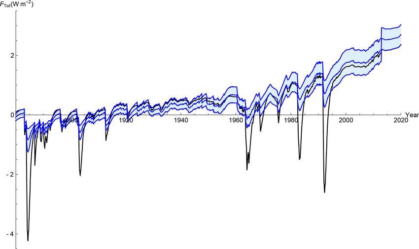
R. Procyk et al.: The fractional energy balance equation for climate projections through 2100                                                      89

Table 1. Model and forcing parameter medians for FEBE calibrated over the historical period (1880–2020) using FAerRCP and FAerSSP , along
with their corresponding 90 % credible intervals.

              Median           h           Median        τ        Median        α           Median         ν            Median           s
                h           90 % CI           τ       90 % CI       α        90 % CI          ν         90 % CI           s           90 % CI
                             range         [years]     range                  range                      range        K[W m−2 ]−1      range
                                                      [years]                                                                       K[W m−2 ]−1
   FAerRCP     0.38        [0.33, 0.44]      4.7     [2.4, 7.0]    0.60       [0.2, 1.0]      0.28     [0.15, 0.41]      0.56       [0.45, 0.67]
   FAerSSP     0.38        [0.32, 0.44]      4.7     [2.4, 7.0]    0.33    [0.05, 0.61]       0.28     [0.16, 0.40]      0.52       [0.43, 0.61]

Table 2. The calculated ECS and TCR medians using both parameters corresponding to FAerRCP and FAerSSP , along with their corresponding
90 % credible intervals.

                                          Median       TCR        Median      ECS             Median        TCR / ECS ratio
                                           TCR        90 % CI      ECS       90 % CI         TCR / ECS       90 % CI range
                                           [K]       range [K]     [K]      range [K]          ratio
                           FAerRCP         1.5       [1.2, 1.8]     2.0     [1.6, 2.4]          0.73           [0.70, 0.78]
                           FAerSSP         1.4       [1.1, 1.6]     1.8     [1.5, 2.2]          0.74           [0.71, 0.79]

3.1     The model: Green’s function parameters: h, τ                          model Green’s function (Held et al., 2010; Geoffroy et al.,
                                                                              2013; IPCC, 2013). Considering G1 (blue), at scales below a
3.1.1    The scaling exponent h                                               few years where the box models or the Hébert et al. (2021)
The model is characterized by h and τ , where the expo-                       truncated scaling model are smooth, the FEBE has a singular
nent h of the FEBE is the most fundamental. For h, we found                   response. This enables it to reproduce the statistics of the in-
a 90 % CI of [0.33, 0.44] shown in Fig. 3a, with a median                     ternal variability as well as to be more sensitive to volcanic
value of 0.38 when using FAerRCP , and while using FAerSSP we                 forcings. Even at scales of up to 25 years, the G1 (blue) re-
found a similar median of 0.38 with 90 % CI of [0.32, 0.44].                  sponds much faster than the IPCC (black), yet the approach
We can already note that it is close to the HEBE value h = 21                 to the asymptotic value of 1 corresponding to energy bal-
and other empirical estimates for power-law impulse Green’s                   ance is substantially slower. This can also be seen in the
functions (G(t) ≈ t −HF −1 ) with h = −HF ≈ 0.5−0.4                           ramp-response Green’s functions (Fig. 4b), G2 , the integral
                                                    +0.5 (Love-
joy et al., 2017; Hébert et al., 2021). The NOAA dataset dif-                 of G1 . For comparison, each was normalized by the value at
fers the most from all others; the exact cause of the difference              70 years – the standard ramp time for TCR (Collins et al.,
is not clear, although it arises from the Merged Land–Ocean                   2013). At multi-year resolution (ignoring the high-frequency
Surface Temperature Analysis (MLOST) dataset’s use of a                       variability), over the scale of the Anthropocene, there is lit-
complex algorithm with low-frequency tuning (Smith et al.,                    tle difference between the FEBE and IPCC, with FEBE hav-
2008). This low-frequency tuning along with the spatiotem-                    ing a more gradual response. This contributes to the some-
poral smoothing applied in the MLOST dataset is likely the                    what cooler FEBE centennial-scale projections when com-
cause of a slightly higher h (i.e. a smoother temperature se-                 pared with those from the two-box model.
ries).
                                                                              3.2      Characterizing the forcing
3.1.2    The relaxation time τ                                                3.2.1        Aerosol linear scaling factor α

The second model parameter is the relaxation time τ that                      The aerosol linear scaling factor α that effectively recali-
characterizes the approach to equilibrium. From the point of                  brates the aerosol forcing (Fig. 5a, solid line) was found to
view of parameter estimation, τ is a difficult parameter to de-               have a median value of 0.6 with a 90 % CI of [0.2, 1.0] for
termine since it is inversely correlated with s: a large τ can                the CMIP5 FAerRCP series. However, when using the CMIP6
be somewhat compensated by a smaller s, and vice versa.                       sulfate-emissions-based aerosol forcing series, FAerSSP , we
As shown in Fig. 3b, we obtained the a posteriori median                      find support for a weaker and better-constrained aerosol
value of 4.7 years and 90 % CI of [2.4, 7.0] years when us-                   forcing, recalibration α with a median of 0.33 and 90 % CI
ing FAerRCP and nearly identical results using FAerSSP .                      of [0.05, 0.61] (Fig. 5a, dashed line). In both cases, an aerosol
   Presented in Fig. 4a is the step-response Green’s func-                    recalibration factor of 1 corresponds to the modern (2005)
tion, G1 (h, τ ; t), of the FEBE with the parameters h and τ                  aerosol forcing value of about −1.0 W m−2 , but we find
along with its 90 % CI, shown alongside the IPCC two-box-                     in both cases that α < 1. The result from two independent

https://doi.org/10.5194/esd-13-81-2022                                                                  Earth Syst. Dynam., 13, 81–107, 2022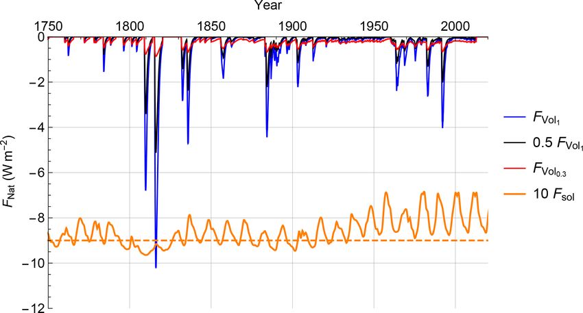
90                               R. Procyk et al.: The fractional energy balance equation for climate projections through 2100

Table 3. Model and forcing parameter medians using FAerRCP for FEBE, the classical continuum mechanics HEBE (h = 21 ) and the SCRF
model (Hébert et al., 2021) calibrated over the historical period, along with their corresponding 90 % credible intervals.

               Median          h          Median        τ        Median          α          Median          ν       Median     ECS
                 h          90 % CI          τ       90 % CI       α          90 % CI         ν          90 % CI     ECS     90 % CI
                             range        [years]     range                    range                      range      [K]      range
                                                     [years]                                                                   [K]
        FEBE       0.38   [0.33, 0.44]      4.7     [2.4, 7.0]       0.6       [0.2, 1.0]    0.28    [0.15, 0.41]     2.0    [1.6, 2.4]
        HEBE        1/2               –     4.7     [2.4, 7.0]      0.48    [0.10, 0.86]     0.33    [0.16, 0.51]     1.8    [1.4, 2.3]
        SCRF        0.5      [0.3, 0.7]     2.0         –            0.8       [0.1, 1.3]    0.55    [0.25, 0.85]     2.3    [1.8, 3.7]

Figure 3. For each observational dataset and their average, PDFs are shown for the model parameters: the scaling parameter h (a) and the
transition time τ (b). Shown are the PDFs for parameter estimation based on both FAerRCP (solid) and FAerSSP (dashed). The average PDF
of the five observation datasets using FAerRCP is shown as the main result with shading, with darker 5 % tails.

aerosol forcing series again shows that the forcing associ-                likely the cause of a lower ν (i.e. a smoother volcanic forc-
ated with aerosols is still widely uncertain and overpowered,              ing).
supporting post-AR5 studies that found aerosol forcings sim-                  In Fig. 6, we compare the total forcing series,
ulated by GCMs were unrealistic (Zhou and Penner, 2017;                    FTot (t) (black), IPCC AR5, Eq. (16), where α = ν = 1, with
Sato et al., 2018; Bellouin et al., 2020) and that aerosol                 the adjusted forcing series, FTot (α, ν; t) (blue). During the
forcing was weaker when climate feedbacks were allowed                     historical period, the intermittency and strength of the strong
(Nazarenko et al., 2017).                                                  volcanic events are greatly reduced, and in the recent past the
                                                                           median-adjusted forcing series is higher than the unadjusted
                                                                           forcing due to the reduced aerosol forcing strength. This ad-
                                                                           justed forcing series consequently contributes to a lower cli-
3.2.2    Volcanic intermittency correction exponent ν                      mate sensitivity, presented in the following section, due to
                                                                           the historic negative forcings of volcanoes and aerosols being
The volcanic intermittency correction exponent ν was found
                                                                           adjusted to closer match historical observations, eliminating
to have a posterior median value of 0.28 with 90 % CI
                                                                           the need for a high climate sensitivity to compensate.
of [0.15, 0.41] when using FAerRCP and similar median
value 0.28 with 90 % CI of [0.16, 0.40] when using FAerSSP
(recall ν = 0 implies a constant mean forcing and the original             3.3     Climate sensitivity
series is recovered with ν = 1). Both contain the theoretically            3.3.1    Climate sensitivity parameter, s
calculated ν within their 90 % CI (ν = 0.32). This result con-
firms that volcanic forcing is generally overpowered since                 The climate sensitivity parameter s refers to the equilib-
ν = 1 has nearly null probability as seen in Fig. 5b. Thus,                rium change in the annual global mean surface temper-
the original volcanic series described without the intermit-               ature (GMST) following a unit change in radiative forc-
tency correction does not reproduce well, within the FEBE                  ing. Its inverse is the climate feedback parameter, the in-
model presented, the cooling events observed in instrumen-                 crease in radiation to space per unit of global warming.
tal records following eruptions: volcanic cooling would be                 We find s to have a median value of 0.56 K(W m−2 )−1
overestimated. As noted in the case for the exponent, h,                   with 90 % CI [0.45, 0.67] K(W m−2 )−1 using FAerRCP , and
the NOAA dataset noticeably differs from the others; the                   when using FAerSSP we find median 0.52 K (W m−2 )−1 with
spatiotemporal smoothing applied in the MLOST dataset is                   90 % CI [0.43, 0.61] K(W m−2 )−1 (Fig. 7), both on the lower

Earth Syst. Dynam., 13, 81–107, 2022                                                            https://doi.org/10.5194/esd-13-81-2022
R. Procyk et al.: The fractional energy balance equation for climate projections through 2100 91
perature response to external forcings in Eq. (7), the climate
sensitivity parameter is the equilibrium climate sensitivity.
The two are equivalent to within a constant factor: the num-
ber of W m−2 per CO2 doubling, the standard value being
3.71 W m−2 /(CO2 doubling) (IPCC, 2013).
The PDF for ECS shown in Fig. 8a, for both aerosols se-
ries, was found to have a 90 % CI of [1.6, 2.4] K and a median
value of 2.0 K when using FAerRCP , and median of 1.8 K and
90 % CI [1.5, 2.2] using FAerSSP (see Table 2). These results
are lower than those found in the CMIP5 MME which had
a best value of 3.2 K, but our 90 % CI bounds are more nar-
row, laying within the CMIP5 MME range of [1.9, 4.5] K.
Although when we consider the expanded ECS 90 % CI of
[1.5, 4.5] K considered in IPCC (2013), which takes into ac-
count both the CMIP5 MME and historical estimates, we
see that the FEBE estimates are wholly within this range
and much less uncertain. For the CMIP6 MME which has
a 90 % CI of [2.0, 5.5] K and mean estimate 3.7 K, our best
estimate using the corresponding FAerSSP is slightly below the
lower credible interval due to the upward shift of ECS esti-
mates seen in CMIP6 models (Zelinka et al., 2020) but again
has a more narrow CI.
3.3.3 Transient climate response
Conventionally, TCR quantifies the temperature change that
would occur if CO2 levels increase by 1 % (compounded) per
Figure 4. (a) The median and 90 % CI of the FEBE step-response year until they double (≈ 70 years). Since the CO2 forcing is
Green’s function, G1 (h, τ ; t), compared to the IPCC two-box- logarithmically dependent on CO2 concentration, the TCR is
model Green’s function (black). (b) The median and 90 % CI of then simply the global temperature increase that has occurred
the FEBE normalized ramp-response Green’s function, G2 (h, τ ; t), at the point in time that a linearly increasing forcing reaches
compared to the IPCC two-box-model Green’s function (black). double pre-industrial levels.
The derived PDFs for TCR are shown in Fig. 8b and sum-
marized in Table 2. Our TCR was found to have a 90 % CI of
end of the CMIP5 MME climate sensitivity parameter of me- [1.2, 1.8] K with a median of 1.5 K when using FAerRCP , while
dian 1 K(W m−2 )−1 and 90 % CI [0.5, 1.5] K(W m−2 )−1 but when using FAerSSP we find a median 1.4 K and 90 % CI of
within the 90 % CI. However, both estimates are below the [1.1, 1.6] K. Both estimates are lower and more constrained
CMIP6 MME 90 % CI [0.63, 1.50] K(W m−2 )−1 , with a me- but within the 90 % CI given by the CMIP5 MME: a 90 % CI
dian of 0.92 K(W m−2 )−1 , which has been criticized as being of [1.2, 2.4] K and a best value of 1.8 K, and by the CMIP6
too high (Zelinka et al., 2020; Tokarska et al., 2020; Flynn MME: 90 % CI of [1.2, 2.8] K with best value of 2.0 K.
and Mauritsen, 2020). The ECS and TCR estimates using the SSP scenarios with
the FEBE are lower than those using RCPs due to the overly
3.3.2 Equilibrium climate sensitivity strong aerosols over the historical period in the SSPs which
require a lower aerosol linear factor along with lower ECS to
Two standard types of climate sensitivity used for inter- best match the historical temperature record. The difference
model comparisons: ECS and TCR – our results are sum- between the shape of the RCP and SSP aerosol forcing can
marized in Table 2. also account for this.
If atmospheric CO2 was increased to double pre-industrial The TCR-to-ECS ratio is a non-dimensional measure of
concentrations and then held there, the planet would only the fraction of committed warming already realized after a
slowly reach a new equilibrium. This delay is largely be- steady increase in radiative forcing; in this case, with a dou-
cause the world’s oceans take a long time to heat up in re- bling of CO2 , this quantity is generally referred to as re-
sponse to the enhanced greenhouse effect. The ECS is the alized warming fraction (RWF) (Stouffer, 2004; Solomon
amount of warming achieved when the entire climate sys- et al., 2009; Millar et al., 2015); it is a non-dimensional mem-
tem reaches “equilibrium” or the steady-state temperature ory parameter. A model with a low RWF will indicate that
response to a doubling of CO2 . By the definition of the tem- global warming may continue for centuries after emissions
https://doi.org/10.5194/esd-13-81-2022 Earth Syst. Dynam., 13, 81–107, 202292 R. Procyk et al.: The fractional energy balance equation for climate projections through 2100
Figure 5. For each observational dataset and their average, PDFs are shown for the forcing parameters: the aerosol scaling factor α (a) and
the volcanic intermittency correction exponent ν (b). Again, shown are the PDFs for parameter estimation based on both FAerRCP (solid) and
FAerSSP (dashed). The average PDF of the five observation datasets using FAerRCP is shown as the main result with shading, with darker 5 %
tails.
Figure 6. The total historical (1880–2020) forcing series prescribed by the IPCC using, FAerRCP (black) compared to the adjusted forcing,
FTot (α, ν; t) (blue), which takes into account aerosol and volcanic corrections, shown with 90 % CI.
have stopped. We present the TCR-to-ECS ratio in Fig. 8c,
with a 90 % CI [0.70, 0.78] and median 0.73 using FRCP pa-
rameters. Similar results are found using FSSP parameters, a
median of 0.72 and 90 % CI [0.71, 0.79]. From Fig. 8 and Ta-
ble 2, we see that the TCR-to-ECS ratio is higher than both
generations of MME 90 % CI, a consequence of lower ECS
and TCR values, and similar uncertainty.
In the next section, we show that with a lower and more
constrained climate sensitivity parameter (Figs. 7 and 8), the
adjusted forcings (Fig. 6) and long memory process of the
FEBE produce future projections that tend to be cooler than
Figure 7. For each observational dataset and their average, PDFs the CMIP5/6 projections, yet remain within their 90 % CI.
are shown for the climate sensitivity parameter s (the ECS, here in
units of K (W m−2 )−1 ), FAerRCP (solid) and FAerSSP (dashed).
Earth Syst. Dynam., 13, 81–107, 2022 https://doi.org/10.5194/esd-13-81-2022You can also read