A framework to evaluate and elucidate the driving mechanisms of coastal sea surface pCO2 seasonality using an ocean general circulation model ...
←
→
Page content transcription
If your browser does not render page correctly, please read the page content below
Ocean Sci., 18, 67–88, 2022
https://doi.org/10.5194/os-18-67-2022
© Author(s) 2022. This work is distributed under
the Creative Commons Attribution 4.0 License.

A framework to evaluate and elucidate the driving mechanisms of
coastal sea surface pCO2 seasonality using an ocean general
circulation model (MOM6-COBALT)
Alizée Roobaert1 , Laure Resplandy2,3 , Goulven G. Laruelle1 , Enhui Liao2 , and Pierre Regnier1
1 Departmentof Geosciences, Environment & Society-BGEOSYS, Université Libre de Bruxelles, Brussels, Belgium
2 Departmentof Geosciences, Princeton University, Princeton, NJ, USA
3 High Meadows Environmental Institute, Princeton University, Princeton, NJ, USA

Correspondence: Alizée Roobaert (alizee.roobaert@ulb.be)

Received: 17 July 2021 – Discussion started: 18 August 2021
Revised: 22 October 2021 – Accepted: 16 November 2021 – Published: 10 January 2022

Abstract. The temporal variability of the sea surface par-        logical and thermal changes. Circulation controls the pCO2
tial pressure of CO2 (pCO2 ) and the underlying processes         seasonality in the Californian Current; biological activity
driving this variability are poorly understood in the coastal     controls pCO2 in the Norwegian Basin; and the interplay
ocean. In this study, we tailor an existing method that quanti-   between biological processes and thermal and circulation
fies the effects of thermal changes, biological activity, ocean   changes is key on the US East Coast. The refined approach
circulation and freshwater fluxes to examine seasonal pCO2        presented here allows the attribution of pCO2 changes with
changes in highly variable coastal environments. We first         small residual biases in the coastal ocean, allowing for fu-
use the Modular Ocean Model version 6 (MOM6) and bio-             ture work on the mechanisms controlling coastal air–sea CO2
geochemical module Carbon Ocean Biogeochemistry And               exchanges and how they are likely to be affected by future
Lower Trophics version 2 (COBALTv2) at a half-degree res-         changes in sea surface temperature, hydrodynamics and bio-
olution to simulate coastal CO2 dynamics and evaluate them        logical dynamics.
against pCO2 from the Surface Ocean CO2 Atlas database
(SOCAT) and from the continuous coastal pCO2 product
generated from SOCAT by a two-step neuronal network
interpolation method (coastal Self-Organizing Map Feed-           1   Introduction
Forward neural Network SOM-FFN, Laruelle et al., 2017).
The MOM6-COBALT model reproduces the observed spa-                The ocean plays an important role in offsetting human-
tiotemporal variability not only in pCO2 but also in sea sur-     induced carbon dioxide (CO2 ) emissions associated with ce-
face temperature, salinity and nutrients in most coastal envi-    ment production and fossil fuel combustion (Friedlingstein
ronments, except in a few specific regions such as marginal       et al., 2019). Globally, the ocean is a net sink that absorbs
seas. Based on this evaluation, we identify coastal regions       roughly one-quarter of the anthropogenic CO2 emitted into
of “high” and “medium” agreement between model and                the atmosphere (−2.5 ± 0.6 petagram of carbon per year
coastal SOM-FFN where the drivers of coastal pCO2 sea-            (Pg C yr−1 ) for the 2009–2018 decade, Friedlingstein et al.,
sonal changes can be examined with reasonable confidence.         2019). The spatiotemporal variability of this oceanic CO2 up-
Second, we apply our decomposition method in three con-           take is relatively well constrained in the open ocean thanks
trasted coastal regions: an eastern (US East Coast) and a         to several methods including sea surface CO2 data-derived
western (the Californian Current) boundary current and a po-      interpolations (e.g., Landschützer et al., 2014; Rödenbeck
lar coastal region (the Norwegian Basin). Results show that       et al., 2014, 2015; Takahashi et al., 2002), models and at-
differences in pCO2 seasonality in the three regions are con-     mospheric inversions (e.g., Gruber et al., 2009, 2019; Keel-
trolled by the balance between ocean circulation and bio-         ing and Manning, 2014; Manning and Keeling, 2006), but

Published by Copernicus Publications on behalf of the European Geosciences Union.
68                                  A. Roobaert et al.: A framework to evaluate and elucidate the driving mechanisms of...

it is less constrained and understood in the coastal ocean.         2013), the southern and southeastern Brazilian shelves, the
Nonetheless, in recent decades, significant progress has been       Uruguayan and Patagonia shelves, and shelves in the SW
made with regard to the quantification and analysis of the          Atlantic Ocean (Arruda et al., 2015). In the California Cur-
spatial distribution of the coastal air–sea CO2 exchange            rent, the strong upwelling of carbon-rich waters was identi-
(F CO2 ) globally and regionally (e.g., Borges et al., 2005;        fied as the main control of the pCO2 seasonality (Turi et al.,
Cai, 2011; Chen et al., 2013; Laruelle et al., 2010, 2014;          2014). On the Patagonia shelf, the thermal effect and bio-
Roobaert et al., 2019). The F CO2 seasonal cycle was also           logical pumps were found to be the main drivers of the sea-
recently analyzed in coastal regions worldwide by Roobaert          sonal pCO2 variability, with only a small contribution from
et al. (2019). This study identified that at the annual timescale   the ocean circulation (Arruda et al., 2015), while along the
the global coastal ocean acts as an atmospheric CO2 sink            US East Coast seasonal thermal changes play the major role
(−0.2 ± 0.02 Pg C yr−1 ), with a more intense CO2 uptake            (Shadwick et al., 2010, 2011; Laruelle et al., 2015; Signorini
occurring in boreal summer because of the disproportionate          et al., 2013). These studies are, however, confined to spe-
contribution of high-latitude coastal regions in the Northern       cific regions and a global picture of the mechanisms driving
Hemisphere, which cover 25 % of the total coastal area and          the coastal pCO2 dynamics is still missing. In addition, the
are characterized by an intense CO2 sink in summer. A more          attribution analysis of specific physical and biological pro-
in-depth analysis also revealed that the majority of the coastal    cesses is incomplete. Indeed, the attribution relies on a linear
seasonal F CO2 variations stems from the air–sea gradient in        decomposition linking variations in sea surface ocean pCO2
partial pressure of CO2 (pCO2 ), although changes in wind           to seasonal changes in DIC, ALK, SST and SSS (e.g., Sig-
speed and sea ice cover can be significant regionally.              norini et al., 2013, Doney et al., 2009; Lovenduski et al.,
   Several processes influence the seasonal variations of sur-      2007; Takahashi et al., 1993; Turi et al., 2014) or on a se-
face ocean pCO2 and thus the seasonality in F CO2 . These           ries of sequential simulations isolating biological and physi-
processes include changes in sea surface temperature (SST)          cal terms and thus ignores how covariations between the dif-
tied to air–sea heat fluxes and ocean circulation, changes in       ferent terms dampen or reinforce each other (e.g., Arruda et
sea surface salinity (SSS) associated with evaporation, fresh-      al., 2015; Turi et al., 2014).
water fluxes (from land, ice melt, precipitation and evapora-          In this study, we develop a new framework to elucidate
tion) and ocean circulation, as well as variations in sea sur-      the seasonal pCO2 dynamics of the global coastal ocean.
face alkalinity (ALK) and dissolved inorganic carbon (DIC)          This framework relies on the global Modular Ocean Model
tied to biological activity, freshwater fluxes and ocean cir-       version 6 (MOM6, Adcroft et al., 2019) from the NOAA
culation (Sarmiento and Gruber, 2006). In the open ocean,           Geophysical Fluid Dynamics Laboratory coupled to the bio-
the respective influence of these processes on the pCO2 vari-       geochemical module Carbon Ocean Biogeochemistry And
ability has been interpreted using changes in SST, SSS, ALK         Lower Trophics version 2 (COBALTv2, Stock et al., 2014,
and DIC observed in situ (e.g., Landschützer et al., 2018;          2020). MOM6-COBALT model outputs provide the relevant
Takahashi et al., 1993) or based on global and regional ocean       variables and processes that are required to perform an ex-
biogeochemical models relying on a mechanistic, quantita-           plicit decomposition of the inorganic carbon dynamics (Liao
tive description of the physical, chemical and biological pro-      et al., 2020) in the entire coastal domain. These outputs are
cesses controlling the ocean carbon cycle (e.g., Doney et al.,      then analyzed using a novel approach to attribute seasonal
2009). These investigations reveal that changes in SST (i.e.,       variations in surface ocean pCO2 to changes in biological ac-
the thermal effect) are the main driver of the seasonal pCO2        tivity, ocean circulation, SST, air–sea CO2 fluxes and fresh-
in tropical oceanic regions, while non-thermal components           water fluxes (Liao et al., 2020) and which is here enhanced
(change associated with DIC, ALK and SSS) dominate at               for the coastal ocean. The decomposition method constitutes
midlatitudes and high latitudes (poleward of 40◦ N and 40◦ S,       a significant improvement upon previous studies. First, it ac-
e.g., Landschützer et al., 2018; Takahashi et al., 2002).           counts for co-variations in biological and physical processes
   In the coastal ocean, the processes controlling the pCO2         and how their evolution jointly modulates the pCO2 signal.
seasonal dynamics were mostly investigated regionally (e.g.,        Second, it improves on the traditional linear approaches de-
Arruda et al., 2015; Frankignoulle and Borges, 2001; Laru-          veloped for the open ocean (Sarmiento and Gruber, 2006;
elle et al., 2014; Nakaoka et al., 2006; Shadwick et al., 2010,     Takahashi et al., 1993) and used since then (e.g. Lovenduski
2011; Signorini et al., 2013; Turi et al., 2014; Yasunaka et al.,   et al., 2007) because, as shown later in this study, the linear
2016), and only a few observation-based studies attempted           decomposition introduces significant biases in coastal waters
to analyze the coastal pCO2 seasonal variability into pro-          due to the larger range in DIC, ALK, pH and salinity values
cesses at the global scale (Cao et al., 2020; Chen and Hu,          encountered in the variable coastal environment (Egleston et
2019; Laruelle et al., 2017). Regional studies using either         al., 2010).
observations or model results have covered, e.g., the shelves          In light of these knowledge gaps, the objective of this pa-
of the entire Atlantic Basin (Laruelle et al., 2014), the US        per are twofold.
West Coast (California Current, Turi et al., 2014), US East
Coast (e.g., Shadwick et al., 2010, 2011; Signorini et al.,

Ocean Sci., 18, 67–88, 2022                                                               https://doi.org/10.5194/os-18-67-2022
A. Roobaert et al.: A framework to evaluate and elucidate the driving mechanisms of...                                          69

    – First, we evaluate the performance of the MOM6-              pogenic carbon content of Khatiwala et al. (2013). At the
      COBALT model in its ability to reproduce the observed        end of an 81-year spin-up repeating the year 1959, the model
      spatiotemporal fields of SSS, SST, sea surface nutrients     reached a near-equilibrium between atmospheric pCO2 and
      and pCO2 in the global coastal domain. In particular,        surface ocean pCO2 , with a drift in global air–sea CO2 flux
      we identify the coastal regions where the model best re-     < 0.004 Pg C yr−1 over the last 10 years of the spin-up. Fur-
      produces the observed ocean pCO2 variability and can         ther details on the configuration, spin-up and simulation can
      thus be considered most suitable for a detailed analysis     be found in Liao et al. (2020).
      of the drivers of the pCO2 seasonal changes.
                                                                   2.2   Observational products and model evaluation
    – Second, to illustrate the capabilities of our upgraded de-
      composition framework, we examine the drivers of the         We first evaluate the ability of MOM6-COBALT to repro-
      pCO2 seasonality in three contrasted coastal regions:        duce the observed spatial distribution of environmental vari-
      the US East Coast, the US West Coast and the Norwe-          ables in the coastal domain, namely the SST, SSS and sea
      gian Basin.                                                  surface nutrients (nitrate, phosphate and silicate). The ob-
                                                                   servational SST and SSS fields are from the daily NOAA
2     Methodology                                                  OI SST V2 (Reynolds et al., 2007) and the daily Hadley
                                                                   center EN4 SSS (Good et al., 2013), respectively. The ob-
2.1    Ocean biogeochemical model description                      served nutrient fields in the sea surface are extracted from
                                                                   the World Ocean Atlas version 2018 (Garcia et al., 2019).
In this study, we used the ocean model MOM6 and the Sea            We also compare the simulated coastal pCO2 directly to un-
Ice Simulator version 2 (fourth generation of ocean ice mod-       interpolated observations extracted from the Surface Ocean
els, OM4) detailed in Adcroft et al. (2019). The version of        CO2 Atlas database (SOCAT) using monthly observations
OM4 adopted here is OM4p5 which has a nominal hori-                from SOCAT version 6 gridded at the spatial resolution of
zontal resolution of 0.5◦ (i.e., with a finer latitudinal reso-    0.25◦ (SOCATv6, Bakker et al., 2016). For the evaluation
lution of 0.26◦ in the tropical region). In the vertical, it in-   period used in this study (1998–2015), this database con-
cludes 75 hybrid coordinates with a z∗ coordinate near the         tains 9.8 million pCO2 observations within the coastal do-
surface (geopotential coordinate allowing free surface undu-       main. All data from SOCATv6 are converted from fugacity
lations) and a modified potential density coordinate below.        of CO2 in water to pCO2 using the formulation of Taka-
The vertical spacing increases from 2 m in the upper 20 m          hashi et al. (2012). We finally compare the pCO2 simu-
(i.e., first 10 layers) to larger isopycnal layers below. Lay-     lated by the MOM6-COBALT model to the 0.25◦ continu-
ers in z∗ broadly deepen towards high latitudes (see Ad-           ous monthly pCO2 fields generated from the SOCAT obser-
croft et al., 2019, for details on the grid). This ocean ice       vations by the two-step neuronal network (Self-Organizing
model is coupled to the biogeochemical module COBALT               Map Feed-Forward neural Network, SOM-FFN) in coastal
version 2 (COBALTv2), which includes 33 state variables to         regions (Laruelle et al., 2017). The SOM-FFN data prod-
resolve global-scale cycles of carbon, nitrogen, phosphate,        uct of Laruelle et al. (2017) is thus not “raw” and implies
silicate, iron, calcium carbonate, oxygen and lithogenic ma-       a significant amount of statistical modeling. It is also derived
terials (Stock et al., 2020). Details about the planktonic food    from an earlier version of SOCAT (SOCATv4, Laruelle et
web dynamics in COBALT, and global assessments of large-           al., 2017) than the one used in this study. In what follows,
scale carbon fluxes through the food web, such as net pri-         the pCO2 products generated by the model, the statistical in-
mary production, can be found in Stock et al. (2014, 2020).        terpolation of observations, and the un-interpolated observa-
The ocean model is forced by the 55 km horizontal resolu-          tions will be referred to as MOM6-COBALT, coastal SOM-
tion Japanese atmospheric reanalysis (JRA55-do) version 1.3        FFN and SOCATv6, respectively. All observational and sim-
at a 3 h frequency between 1959 and 2018 (Tsujino et al.,          ulated fields are converted from their original spatiotempo-
2018), and the atmospheric CO2 concentration data (xCO2 )          ral resolution to monthly 0.25◦ gridded climatologies for the
from the Earth System Research Laboratory (Conway et al.,          1998–2015 period to match the one used by the coastal SOM-
1994; Masarie, 2012). The xCO2 is converted to pCO2 using          FFN. Cells that are covered by more than 95 % sea ice are re-
atmospheric and water vapor pressures by the model. SST,           moved from the comparison since we assume no transfer of
SSS, sea surface nutrients (nitrate, phosphate, silicate) and      our master variable (pCO2 ) through sea ice. In our analysis,
oxygen were initialized from the World Ocean Atlas ver-            we apply the broad definition of the coastal zone by Laruelle
sion 2013 (Garcia et al., 2013a, b; Locarnini et al., 2013;        et al. (2017), using a global mask that excludes estuaries and
Zweng et al., 2013). Initial DIC and ALK conditions are            inland water bodies, while its outer limit is set 300 km away
taken from GLODAPv2 (Olsen et al., 2016). The initial DIC          from the shoreline. This definition leads to a total surface
is corrected for the accumulation of anthropogenic carbon          area of 77 million km2 , which is split into 45 coastal regions
to match the level expected in the first year of the simula-       using the MARgins and CATchment Segmentation (MAR-
tion (1959) using the data-based estimate of ocean anthro-         CATS, Laruelle et al., 2013). These 45 regions are grouped

https://doi.org/10.5194/os-18-67-2022                                                               Ocean Sci., 18, 67–88, 2022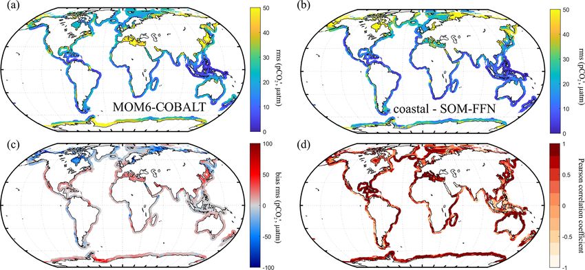
70                                 A. Roobaert et al.: A framework to evaluate and elucidate the driving mechanisms of...

into seven broad classes with similar hydrological and cli-       “high” when the three criteria are fulfilled, “medium” when
matic settings (Liu et al., 2010): (1) an Eastern Boundary        criteria 2 and 3 are satisfied, and “low” when only one (or
Current and (2) Western Boundary Current (EBC and WBC,            no) criterion is met for the seasonality.
respectively), (3) tropical margins, (4) subpolar and (5) polar
margins, (6) marginal seas, and (7) Indian margins.               2.3   Processes controlling seasonal pCO2 variability: a
   The model evaluation of all gridded environmental vari-              method tailored for coastal regions
ables including pCO2 is performed for the annual mean
and the seasonal cycle both globally and within each of           The pCO2 in surface sea water can be computed from DIC
the 45 MARCATS regions. For the seasonal analysis a cli-          and ALK following Eq. (1) (Sarmiento and Gruber, 2006;
matological monthly anomaly is calculated, for each vari-         Wolf-Gladrow et al., 2007):
able, as the difference between the variable x for a given                  K20 (2DIC − ALK)2
month and its climatological annual mean. The evaluation          pCO2 =                      ,                              (1)
                                                                           K00 K10 ALK − DIC
of the seasonal amplitude is then performed using the bias
between observed and simulated root mean square (rms) of          where K00 is the aqueous-phase solubility constant of CO2
their monthly anomalies. A positive bias represents a larger      in water and K10 and K20 represent the apparent equilibrium
simulated seasonal amplitude than derived from the observa-       dissociation constants of the carbonate system. Several phys-
tions. The temporal shift between the observed and simulated      ical and biogeochemical processes can thus affect pCO2 via
                                                                                                           K0
seasonal cycles is also assessed from the Pearson correla-        changes in DIC, ALK and/or via the K 0 K2 0 term, which de-
                                                                                                           0 1
tion coefficient (no units) of the regression between monthly     pends on SST and SSS. To quantify the processes control-
times series simulated by MOM6-COBALT and those ex-               ling the pCO2 variability at the seasonal timescale of inter-
tracted from the observations. These comparisons not only         est to this study, we adopt the method of Liao et al. (2020).
serve to assess the overall model performance in reproducing      The method starts from the traditional approach that links
observations but also help to identify potential discrepancies    variations in sea surface ocean pCO2 to changes in DIC,
between observed and simulated environmental fields (e.g.,        ALK, SST and SSS using the following linear decomposi-
SST, SSS) that are used by the two-step neuronal network          tion (Doney et al., 2009; Lovenduski et al., 2007; Takahashi
coastal SOM-FFN to generate the continuous pCO2 clima-            et al., 1993; Turi et al., 2014):
tology. We use two metrics to evaluate SOCATv6 spatial and                     ∂pCO2             ∂pCO2
temporal coverage. First, we evaluate the spatial coverage at     1pCO2 ≈              1DIC +          1ALK
                                                                                ∂DIC              ∂ALK
the MARCATS region scale by computing the percent sur-
                                                                               ∂pCO2             ∂pCO2
face area sampled by SOCATv6 data for each MARCATS re-                      +         1SST +           1SSS,                 (2)
gion. A 50 % spatial coverage means that SOCATv6 data are                       ∂SST              ∂SSS
available in 50 % of the 0.25◦ × 0.25◦ cells included in this     where 1x terms represent the seasonal anomaly of x (i.e.,
specific MARCATS region (this metric is used in Fig. 1a).         the departure from the annual mean) and ∂pCO        2  ∂pCO2
                                                                                                                  ∂DIC , ∂ALK ,
                                                                  ∂pCO2        ∂pCO2
Second, we evaluate the ability of SOCATv6 to capture the          ∂SST and ∂SSS are coefficients that describe the sensitivity
seasonality at the grid cell scale by computing the number of     of pCO2 to changes in DIC, ALK, SST and SSS, respec-
months where there is at least one SOCATv6 pCO2 measure-          tively. The coefficients for DIC, SST and SSS are always
ment for each 0.25◦ × 0.25◦ grid cell. An 8-month temporal        positive as pCO2 increases with increases in DIC, SST or
coverage means that 8 out of the 12 months are sampled at         SSS, while the coefficient for ALK is always negative as
least once in this grid cell (this metric is used in Fig. 6a).    pCO2 systematically decreases with increasing ALK. These
   Finally, from this global and regional spatiotemporal eval-    coefficients are generally estimated using the approach of
uation, we label the agreement between the model and              Sarmiento and Gruber (2006) (see Eqs. S1–S4 in the Supple-
coastal SOM-FFN (“high”, “medium” and “low”) for each             ment), which has been widely used in the open ocean (Liao
MARCATS region and identify regions for which our re-             et al., 2020; Sarmiento and Gruber, 2006; Takahashi et al.,
sults are the most robust for further in-depth analysis of        1993). In this study, we refine the estimation of the coeffi-
the processes driving the coastal pCO2 dynamics. The la-          cients so they can be used for the wide range of DIC / ALK
bels of agreement are based on three criteria. First, we assess   ratios that can be encountered in the coastal waters. This in-
whether the simulated annual mean pCO2 is within 20 µatm          cludes conditions when the DIC / ALK ratio is close to 1,
of the one extracted from the coastal SOM-FFN. This thresh-       such as in regions with significant freshwater discharge like
old of 20 µatm roughly corresponds to the globally averaged       those found near estuarine mouths or on polar shelves sub-
pCO2 gradient between the atmosphere and the coastal sea          ject to sea ice melting when pH is around 7.5 (Egleston et al.,
surface (Laruelle et al., 2018). The second and third criteria    2010). In these cases, the traditional approximation method
evaluate the magnitude and phasing of the simulated pCO2          using mean DIC, ALK, SSS and SST fields breaks down
seasonal cycle against the coastal SOM-FFN using an abso-         (see Eqs. S1–S2 and Fig. S1 in the Supplement). To cir-
lute bias in the seasonal magnitude  0.5 as a threshold. The agreement is considered     cients of the pCO2 dependency using a regression approach

Ocean Sci., 18, 67–88, 2022                                                            https://doi.org/10.5194/os-18-67-2022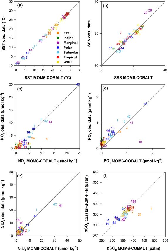
A. Roobaert et al.: A framework to evaluate and elucidate the driving mechanisms of...                                                    71

Figure 1. (a) SOCATv6 spatial coverage (color) and agreement between model and coastal SOM-FFN product (symbols) in coastal MAR-
CATS (Margins and CATchment Segmentation) regions. The blue intensity indicates the fraction of the MARCATS region’s surface area
covered by SOCATv6 observations (from light to dark blue). Dots indicate where the model fulfills three evaluation criteria (“high” agreement
regions) of the spatiotemporal pCO2 distribution (i.e., annual mean mismatch  0.5, and seasonal amplitude mismatch
72                                    A. Roobaert et al.: A framework to evaluate and elucidate the driving mechanisms of...

Table 1. Model vs. coastal SOM-FFN agreement level. For each MARCATS region, the agreement (“high”, “medium” and “low”) is at-
tributed by the pCO2 spatiotemporal analysis. Regions where the model fulfills criteria on the annual mean and seasonality are labeled
as high-agreement regions (i.e., annual mean mismatch 0.5, and seasonal amplitude mismatch 20 µatm on the
comparison with SOCATv6 (see Table S1 in the Supplement). Medium-agreement regions represent MARCATS regions where the model
only fulfills seasonal criteria (seasonal amplitude and phase, dashed in Fig. 1a). Other regions (low agreement) do not fulfill the two criteria
associated with the seasonality (no symbol in Fig. 1a). Regions with high agreement are considered the most robust for an in-depth analysis
of the processes driving the coastal pCO2 dynamics and are highlighted in bold.

                                                                Annual mean pCO2 (µatm)              Seasonal pCO2
                                                                                             Amplitude (µatm)
 MARCATS        MARCATS                        MARCATS               Coastal       Model      Coastal    Model       Phasing     Model vs.
 number (Mx)    name                           category         SOM-FFN rms         bias    SOM-FFN       bias      (Pearson     coastal SOM-FFN
                                                                                                                  coefficient)   agreement
 2              Californian Current            EBC                       360.0      34.5          8.3     16.2           1.0     Medium
 4              Peruvian Upwelling Current     EBC                       377.6     106.4          4.1      6.6          −0.4     Low
 19             Iberian upwelling              EBC                       354.8       9.3          7.5     15.6           0.8     High
 22             Moroccan upwelling             EBC                       379.4      10.2          7.4      8.7           0.9     High
 24             SW Africa                      EBC                       349.1      79.3          7.2      4.2           0.9     Medium
 33             Leeuwin Current                EBC                       349.4       4.2          5.6     12.7           0.9     High
 27             W Arabian Sea                  Indian margins            383.5      11.6          8.7      3.6           0.3     Low
 30             E Arabian Sea                  Indian margins            388.4      −8.3          4.8      6.2           0.7     High
 31             Bay of Bengal                  Indian margins            377.3     −24.1          7.4     13.5          −0.2     Low
 32             Tropical E Indian Ocean        Indian margins            373.3       0.3          2.3      5.4           0.9     High
 9              Gulf of Mexico                 Marginal sea              384.3      −9.1         13.9     12.9           1.0     High
 12             Hudson Bay                     Marginal sea              326.4       5.7         65.3    −46.4           0.4     Low
 18             Baltic Sea                     Marginal sea              336.2      21.4         79.4    −44.4           0.9     Low
 20             Mediterranean Sea              Marginal sea              388.1     −11.9         25.1     20.6           1.0     Low
 21             Black Sea                      Marginal sea              325.0      25.2        141.9   −116.9          −0.5     Low
 28             Red Sea                        Marginal sea              412.2     −16.5         25.0     −0.4          −0.9     Low
 29             Persian Gulf                   Marginal sea              411.2      −7.6         31.3     30.7          −0.9     Low
 40             Sea of Japan                   Marginal sea              330.3      −9.3         21.1     28.0           0.9     Low
 41             Sea of Okhotsk                 Marginal sea              321.2      29.2         28.6     −6.5           0.7     Medium
 13             Canadian Archipelago           Polar                     325.4     −53.1         43.4    −18.0           0.9     Medium
 14             N Greenland                    Polar                     306.0     −24.3         21.7     −9.0           0.8     Medium
 15             S Greenland                    Polar                     325.2       1.3         24.5     −8.5           1.0     High
 16             Norwegian Basin                Polar                     328.1      −0.7         19.9     −6.1           0.9     High
 43             Siberian shelves               Polar                     338.2     −19.7         57.4    −15.7           0.9     High*
 44             Barents and Kara seas          Polar                     311.6      −3.3         24.9     −7.4           0.7     High
 45             Antarctic shelves              Polar                     373.7     −17.6         22.6     13.3           1.0     High*
 1              NE Pacific                     Subpolar                  342.5      16.8         15.8     −4.5           0.8     High*
 5              South America                  Subpolar                  351.1      14.0         12.1     −6.4           0.8     High
 11             Sea of Labrador                Subpolar                  326.3       5.5         17.0      0.8           0.2     Low
 17             NE Atlantic                    Subpolar                  354.4      −4.5         14.9     −8.2           0.6     High
 34             S Australia                    Subpolar                  352.7      13.5          3.7     12.8           0.9     High
 36             New Zealand                    Subpolar                  352.4       6.1          2.6      6.2          −0.5     Low
 42             NW Pacific                     Subpolar                  337.7      25.2         36.5    −19.2           1.0     Medium
 3              Tropical E Pacific             Tropical                  382.2      17.2          6.9      3.1           0.3     Low
 7              Tropical W Atlantic            Tropical                  380.3     −19.8          2.8      9.6           1.0     High
 8              Caribbean Sea                  Tropical                  387.6      −1.7          6.6      2.2           1.0     High
 23             Tropical E Atlantic            Tropical                  374.6      15.9          2.9      1.5           0.6     High*
 26             Tropical W Indian Ocean        Tropical                  384.8       4.8          7.1      5.6           0.9     High*
 37             N Australia                    Tropical                  378.5      −4.0          4.3      5.2           1.0     High
 38             SE Asia                        Tropical                  373.5       0.6          2.6      8.9           0.2     Low
 6              Brazilian Current              WBC                       374.8       7.0          6.7      7.5           0.9     High
 10             US East Coast                  WBC                       368.1      −9.6         12.0     12.4           0.9     High
 25             Agulhas Current                WBC                       367.1       5.7          7.1      8.1           1.0     High
 35             E Australian Current           WBC                       343.9       2.9          3.3      7.4           1.0     High
 39             East China Sea and Kuroshio    WBC                       359.6      −4.1         10.3     13.2           0.9     High

Ocean Sci., 18, 67–88, 2022                                                                       https://doi.org/10.5194/os-18-67-2022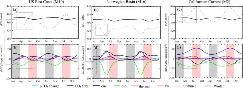
A. Roobaert et al.: A framework to evaluate and elucidate the driving mechanisms of...                                                                      73

based on the CO2SYS program (Lewis and Wallace, 1998).            SST (∂t SST) and SSS (∂t SSS):
At each point in space, pCO2 was computed using the 1998–
                                                                                 ∂pCO2          ∂pCO2
2015 average of DIC, ALK, SSS and SST with CO2SYS                 ∂t pCO2 ≈            ∂t DIC +       ∂t ALK
(method 14 in the CO2SYS MATLAB program, Millero,                                 ∂DIC           ∂ALK
2010). The ∂pCO   2                                                              ∂pCO2          ∂pCO2
              ∂DIC coefficient was then computed as the slope                  +       ∂t SST +       ∂t SSS.                                               (3)
of the linear regression between pCO2 and DIC obtained by                         ∂SST           ∂SSS
allowing DIC to vary around the local mean DIC value while        Temporal changes in DIC, ALK, SST and SSS (∂t DIC,
keeping other tracers (ALK, SST, SSS) constant. The DIC           ∂t ALK, ∂t SST and ∂t SSS) are controlled by surface heat flux,
range used to compute the slope was set to the ± 2 SD of          ocean transport, freshwater fluxes, biological processes and
the 1998–2015 monthly values at that location with an up-         the air–sea CO2 flux. Using the model results, we further ex-
per bound at ± 60 µmol kg−1 (see the Supplement for fur-          pand the decomposition to quantify the contribution of these
ther details). The same approach was repeated to compute          physical and biological processes (see Liao et al, 2020, for
the coefficients for the pCO2 dependence on ALK, SST and          details about the derivation):
SSS, respectively. Our methodology leads to coefficients that
are constant in time but are space dependent. In Fig. S1, we          ∂t pCO2 ≈
                                                                      | {z }
compare the coastal pCO2 reconstructed from the traditional       pCO2 change
decomposition (using the space-varying coefficients reported
                                                                    ∂pCO2           ∂pCO2           ∂pCO2            ∂pCO2           ∂pCO2           ∂pCO2

                                                                          ∂t DICh +       ∂t ALKh +       ∂t SSSh +        ∂t DICv +       ∂t ALKv +       ∂t SSSv
by Sarmiento and Gruber, 2006) with those computed here           |
                                                                     ∂DIC           ∂ALK             ∂SSS
                                                                                                                  {z
                                                                                                                      ∂DIC           ∂ALK             ∂SSS
                                                                                                                                                                   }
using the CO2SYS regression. For the global coastal ocean,
                                                                                                                 circ

we find a large bias (global mean root-mean-square error              ∂pCO2            ∂pCO2            ∂pCO2
                                                                  +         ∂t DICfw +       ∂t ALKfw +       ∂t SSSfw
(RMSE) of fitting pCO2 anomaly in Eq. (2) = 14.6 µatm),                ∂DIC            ∂ALK              ∂SSS
which is especially pronounced at high latitudes. In contrast,      |                       {z                         }
                                                                                                                  fw
the decomposition method based on our methodology dras-
                                                                      ∂pCO2              ∂pCO2
tically reduce the biases (global mean RMSE = 2.8 µatm) in        +         ∂t DICbio +        ∂t ALKbio
coastal regions and allows a more robust reconstruction of             ∂DIC              ∂ALK
                                                                    |                 {z                 }
the pCO2 variability.                                                                              bio
   We further evaluated how using coefficients that vary in

                                                                      ∂pCO2
both time and space could reduce the residual biases be-          +         ∂t SSTh + ∂t SSTv + ∂t SSTq
                                                                       ∂SST
tween our pCO2 decomposition (using space-dependent co-             |               {z                    }
                                                                                                 thermal
efficients that are constant in time) and the pCO2 simulated
in the model that are found in regions with large freshwater             ∂pCO2
                                                                  +            ∂t DICCO2 flux ,
discharge, such as the mouth of the Amazon River or Arctic                ∂DIC
                                                                       |          {z         }
coastal waters. We compare the pCO2 seasonality simulated                           CO2 flux
by the model to the pCO2 reconstructed by the following                                                                                                     (4)
three methods: space-varying coefficients from Sarmiento
and Gruber (2006), regression-based space-varying coeffi-         where the temporal changes in pCO2 (time tendency called
cients, and regression-based space- and time-varying coeffi-      pCO2 change) are on the left-hand side (LHS) of the equa-
cients, all of which used a point in the Amazon River plume       tion and the five terms that control this change in pCO2 are
(1◦ N, 310.25◦ E, Fig. S1d and e). At this location, the use      on the right-hand side (RHS) of the equation. Subscripted
of the regression-based coefficients greatly improves the re-     h and v denote the contribution from horizontal (advec-
covery of the simulated pCO2 compared to using the tradi-         tion and diffusivity in the meridional and zonal directions)
tional coefficients of Sarmiento and Gruber (2006), reducing      and vertical (vertical advection and diffusivity) transports
the RMSE from 83 to 24 µatm, corresponding to a bias re-          on SST, SSS, DIC, and ALK; “bio” denotes the DIC and
duction of 71 %. The use of both space- and time-dependent        ALK changes induced by biological processes (photosynthe-
regression-based coefficients further reduces this bias, bring-   sis, respiration, calcium carbonate dissolution and precipita-
ing down the RMSE from 24 to 18 µatm corresponding to an          tion, denitrification, and nitrification); q denotes the effect of
additional 7 % reduction of the initial bias (83 µatm). Based     surface heat flux on SST; “fw” denotes the effect of fresh-
on these results, we chose to use space dependent only coef-      water fluxes (i.e., precipitation, evaporation, river runoff, and
ficients, which is a simpler approach to implement here and       sea ice formation and melting) on SSS, DIC, and ALK; and
in future studies.                                                the term CO2 flux denotes the DIC change induced by air–sea
   Here we assume that the coefficients are constant in           CO2 exchange.
time, and the temporal change in pCO2 (∂t pCO2 in                    Here we examine changes in pCO2 attributed to three
µatm per month) can therefore be expressed as a simple func-      oceanic processes that modify the concentration in dissolved
tion of the temporal changes in DIC (∂t DIC), ALK (∂t ALK),       species (i.e., DIC, ALK and SSS), namely their transport by
                                                                  oceanic circulation (“circ”, which includes horizontal and

https://doi.org/10.5194/os-18-67-2022                                                                               Ocean Sci., 18, 67–88, 2022
74 A. Roobaert et al.: A framework to evaluate and elucidate the driving mechanisms of...
vertical transport), the effect of dilution and concentration lantic (M17) to 1.3 ◦ C on the US East Coast (M10, Fig. 3a
due to freshwater fluxes (fw), and the effect of biological ac- and Table S1). With a global median bias value of 0.2, the
tivity (bio), and these processes isolate the thermal influence model also correctly reproduces the observed SSS patterns
tied to SST changes induced by both oceanic transport and that are mainly regulated by evaporation and freshwater in-
air–sea exchange of heat. Finally, the air–sea CO2 exchange puts from precipitation, riverine runoff and ice melt, with
(CO2 flux) pushes the surface pCO2 concentration towards lower SSS values in polar regions and along the coasts of
its equilibrium with the atmosphere and systematically acts Southeast Asia and higher SSS values along the coasts of
to offset the pCO2 changes associated with the sum of the evaporation basins such as in the Arabian Sea or the Mediter-
internal oceanic processes (circ, bio, fw and thermal). In this ranean Sea (Fig. 2d–f). The SSS analysis at the MARCATS
study, we apply Eq. (4) using averages between the sea sur- scale reveals absolute SSS biases that are generally less than
face and the mixed-layer depth (MLD), defined here as the or close to 1, except for five MARCATS regions where ab-
depth where the water density is 0.01 kg m−3 denser than the solute biases exceed 2. These MARCATS regions are mainly
water at the surface (minimum MLD is 5 m). Positive contri- located in marginal seas (the Baltic Sea, M18; the Black Sea,
butions on the RHS would yield an increase in pCO2 (posi- M21; and the Persian Gulf, M29) but also include one po-
tive pCO2 response on the LHS). Positive values of the CO2 lar region (the Canadian Archipelago, M13) and one tropi-
flux correspond to an ocean CO2 uptake. This method to de- cal region (Tropical West Atlantic, M7; see Fig. 3b and Ta-
compose the pCO2 seasonality into controlling processes in ble S1). Similar to SSS, largest the model–data discrepancies
the coastal domain is illustrated in three coastal regions: the for nutrients are mostly found in marginal seas (Fig. 3c–e
US East Coast, the US West Coast and the Norwegian Basin. and Table S1). For instance, the largest PO4 and SiO4 bi-
ases are encountered in the Black Sea (M21, absolute bi-
ases of 3 and 75 µmol kg−1 , respectively). The Peruvian Up-
3 Results and discussion welling Current (M4), the Bay of Bengal (M31) and the NE
Pacific (M1) also present large biases in NO3 and PO4 (e.g.,
3.1 Annual mean state and seasonal cycle model
NO3 bias of 8 µmol kg−1 for M4). However, the global me-
evaluation and identification of coastal regions
dian nutrients biases are much smaller, reaching 0.3, −0.2
Figure 1a identifies the coastal regions where the perfor- and −0.4 µmol kg−1 for nitrate (NO3 , Fig. 2i), phosphate
mance of MOM6-COBALT is satisfactory for both the an- (PO4 , Fig. 2l) and silicate (SiO4 , Fig. 2o), respectively.
nual mean and the seasonal cycle of pCO2 . The analysis, The model–data seasonal evaluation reveals that MOM6-
performed at the MARCATS scale (see Fig. 1b for nomencla- COBALT reproduces the global SST and SSS amplitudes re-
ture), distinguishes regions of low, medium and high agree- markably well (median absolute bias of 0.1 ◦ C and 0.0, re-
ment between the model and coastal SOM-FFN, the latter spectively; see Table S2 in the Supplement). Some excep-
being areas for which our confidence in the identification of tions can nevertheless be diagnosed, such as in the marginal
the dominant biophysical drivers of the coastal pCO2 dy- Black Sea (M21), where the bias in SST seasonal ampli-
namics is highest. This figure will be analyzed in detail in tude reaches −1.3 ◦ C, and in three MARCATS regions (Bay
Sect. 3.1.3, but before we do so we first perform a data– of Bengal, M31; tropical West Atlantic, M7; and Siberian
model evaluation according to the following procedure. We shelves, M43) where the SSS seasonal biases are larger
first evaluate the model by comparing simulated fields of than 0.4. The model–data comparison also reveals that the
SSS, SST and sea surface nutrients to global and regional ob- phasing of the SST and SSS seasonal cycles are in very
servations (Sect. 3.1.1, Figs. 2 and 3). Second, the ability of good agreement (Pearson correlation close to 1) for all 45
the model to capture the coastal pCO2 annual mean and sea- MARCATS regions, with the exception of four for which
sonality is assessed against the SOCATv6 data and the con- significant deviations in SSS are found, i.e., two marginal
tinuous monthly observation-based pCO2 product (coastal seas (Hudson Bay, M12, and the Red Sea, M28) and along
SOM-FFN, Laruelle et al., 2017; see Sect. 3.1.2 and Figs. 3– the Californian Current (M2) and Brazilian Current (M6).
6). The nutrients analysis shows absolute global median bi-
ases in seasonal amplitude of 0.1, 0.0 and 0.7 µmol kg−1
3.1.1 Model evaluation for coastal waters for NO3 , PO4 and SiO4 , respectively. Seven MARCATS re-
environmental variables gions present absolute biases larger than 1.5 µmol kg−1 that
are mainly located in marginal seas (Baltic Sea, M18; Sea
MOM6-COBALT captures the main spatial patterns of key of Japan M40; and Sea of Okhotsk, M41) but also in po-
environmental parameters (SST, SSS and sea surface nutri- lar (Siberian, M43, and Antarctic, M45, shelves) and sub-
ents) fairly well in the coastal domain (Fig. 2). The global polar (NE Pacific, M1) regions and in the Bay of Ben-
SST field simulated by the model reproduces the strong gal (M31). The model–data comparison sometimes shows
large-scale tropical to polar SST gradients, with a global significant phase shifts in their seasonal signal (Pearson co-
median bias of −0.2 ◦ C (Fig. 2a–c), and biases at the scale efficient < 0.5), such as for MARCATS regions located in
of MARCATS regions ranging from 0 ◦ C in the NE At- Indian and tropical margins, marginal seas, and EBCs.
Ocean Sci., 18, 67–88, 2022 https://doi.org/10.5194/os-18-67-2022A. Roobaert et al.: A framework to evaluate and elucidate the driving mechanisms of... 75
Figure 2. Observed (center) and modeled (left) spatial distributions of the annual mean state of SST (◦ C), SSS (no unit), nitrate (NO3 ,
µmol kg−1 ), phosphate (PO4 , µmol kg−1 ) and silicate (SiO4 , µmol kg−1 ) and model annual mean bias (right). Observational SST and SSS
fields are from the NOAA OI SST V2 (Reynolds et al., 2007) and the EN4 SSS (Good et al., 2013). Observational nutrients are from the
World Ocean Atlas version 2018 (Garcia et al., 2019). The bias is the difference between MOM6-COBALT and observed values (red indicates
regions where the simulated variables by MOM6-COBALT exceed observed values).
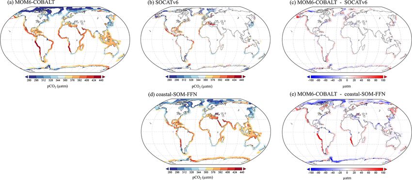
3.1.2 Model evaluation for coastal pCO2 that in some MARCATS regions, in particular in marginal
seas and Indian seas, there are no SOCATv6 observations to
perform the comparison (e.g., the Bay of Bengal, M31; see
The spatial distribution of the annual mean pCO2 simulated
Fig. 4b and Table S1). Hence, we also evaluate the perfor-
by MOM6-COBALT is in good agreement with the observa-
mance of MOM6-COBALT against the continuous coastal
tional pCO2 values extracted from the SOCATv6 database
SOM-FFN pCO2 product, which uses a neural network inter-
with generally low pCO2 values (blue colors) in temperate
polation method to fill data gaps and resolve the spatiotem-
and high latitudes and high pCO2 values (yellow and red
poral coastal pCO2 variability globally.
colors) in tropical and sub-tropical regions (Fig. 4a–c). The
Our results show that MOM6-COBALT reproduces the
model–data pCO2 evaluation at the regional scale shows that
main spatial features of the annual mean pCO2 field cap-
33 of the 45 MARCATS present absolute biases lower than
tured by the coastal SOM-FFN product, as revealed by the
20 µatm (Table S1). The regions where the bias exceeds this
relatively low globally averaged bias of 2.5 µatm (Fig. 4a and
threshold include two EBCs (the Californian Current, M2,
d). In both the model and the SOM-FFN product, low coastal
and the Peruvian Upwelling Current, M4), two marginal seas
pCO2 values are consistently found in temperate and high-
(Sea of Japan, M40, and Sea of Okhotsk, M41), and one polar
latitude regions in both hemispheres, while high pCO2 val-
region (Antarctic shelves, M45), a subpolar region (NW Pa-
ues are largely limited to (sub-)tropical regions. The largest
cific, M42) and the tropical East Atlantic (M23) shelf. Note
https://doi.org/10.5194/os-18-67-2022 Ocean Sci., 18, 67–88, 202276 A. Roobaert et al.: A framework to evaluate and elucidate the driving mechanisms of...
At the regional scale, differences in annual mean pCO2
between MOM6-COBALT and coastal SOM-FFN are lower
than 20 µatm in 35 MARCATS (Table S1, Fig. 3f), which
partly is a reflection of the low annual mean biases ob-
served in the environmental driver variables in these regions
(see Sect. 3.1.1). In EBC, WBC and subpolar coastal re-
gions, the model tends to overestimate the regional mean
pCO2 compared to coastal SOM-FFN (positive bias), except
along the US East Coast (M10), in the East China Sea and
Kuroshio (M39), and in the NE Atlantic (M17, Table S1).
In polar regions, the model generally underestimates the
mean pCO2 compared to coastal SOM-FFN, except around
S Greenland (M15). In Indian, marginal, and tropical coastal
regions, no general trend can be identified regarding the sign
of the bias, which can be positive or negative.
Quantitatively, the 10 MARCATS regions with absolute
biases > 20 µatm are mainly located in regions for which
very limited or no observational data have been compiled in
the SOCATv6 database (Table S1) and/or for which large dis-
crepancies can already be identified at the level of the master
environmental variables (Sect. 3.1.1). These regions mainly
belong to EBCs (three out of the six EBC MARCATS re-
gions) and marginal seas (three out of the nine marginal seas
MARCATS regions), with the remaining four being either
polar (the Canadian Archipelago, M13, and the N Green-
land, M14), subpolar (NW Pacific, M42) or Indian margins
(the Bay of Bengal, M31). The largest biases are found in
the Peruvian Upwelling Current (M4), SW Africa (M24),
the Californian Upwelling Current (M2) and the Canadian
Archipelago (M13), with biases of 106, 79, 35 and −53 µatm,
Figure 3. Comparison between observed and simulated annual respectively.
mean fields in the 45 MARCATS regions: (a) SST (◦ C), (b) SSS Our analysis reveals that the seasonal amplitudes simu-
(no unit), (c) NO3 (µmol kg−1 ), (d) PO4 (µmol kg−1 ), (e) SiO4 lated by MOM6-COBALT are systematically larger than the
(µmol kg−1 ) and (f) pCO2 (µatm). Observational datasets are as ones estimated by the coastal SOM-FFN product (Fig. 5a–
follows: SST and SSS are from the NOAA OI SST V2 (Reynolds b, red colors in Fig. 5c and positive biases in Table S2) for
et al., 2007) and the EN4 SSS (Good et al., 2013), nutrients are all coastal regions belonging to EBC, WBC, and Indian and
from the World Ocean Atlas 2018 (Garcia et al., 2019), and pCO2 tropical margins. For the majority of the polar and subpo-
is from the coastal SOM-FFN product (Laruelle et al., 2017). Col-
lar margins and for some marginal seas, the model simu-
ors correspond to the seven major MARCATS classes (see Fig. 1b).
lates lower seasonal pCO2 amplitudes (blue colors in Fig. 5c
In panels (d) and (e), the Black Sea (M21) is not represented and
has xy coordinates of (0.2; 3.5 µmol kg−1 ) in panel (d) and (10.3; and negative biases in Table S2). Quantitatively, absolute bi-
83.1 µmol kg−1 ) in panel (e). The Antarctic shelf (M45) is also not ases between the modeled and coastal SOM-FFN amplitudes
represented in panel (e) (55.0;49.1 µmol kg−1 ). do not exceed 20 µatm, except for in marginal seas where
larger discrepancies are calculated (six of the nine marginal
MARCATS regions, Table S2). The monthly mean pCO2
discrepancies (Fig. 4e) are found at high latitudes (poleward seasonal cycle simulated by MOM6-COBALT is also well
of 60◦ N and 60◦ S, negative bias), along the Peruvian and in phase (Pearson correlation coefficients > 0.5) with the
Namibian upwelling systems (high positive bias) and more one extracted from coastal SOM-FFN in 34 out of the 45
locally close to the mouth of some large rivers (e.g., the MARCATS regions (Fig. 5d and Table S2). The agreement
plume of the Amazon or the Rio de la Plata, high nega- is especially good in the best-monitored MARCATS regions
tive bias). We note, however, that these regions are poorly (MARCATS where > 50 % of the area is covered by SO-
sampled in the SOCATv6 dataset (Fig. 4b) and are thus CATv6 observations, Table S1). For instance, in regions with
likely weakly constrained in the coastal SOM-FFN product good data coverage, such as along the US East Coast (M10),
(Fig. 4d). the Norwegian Basin (M16), the Californian Current (M2),
the Leeuwin Current (M33) or the Brazilian Current (M6),
the Pearson correlation coefficient is higher than 0.9 (Ta-
Ocean Sci., 18, 67–88, 2022 https://doi.org/10.5194/os-18-67-2022A. Roobaert et al.: A framework to evaluate and elucidate the driving mechanisms of... 77
ble S2). In contrast, the seasonal pCO2 cycle simulated gions that are best covered by observations (MARCATS re-
by MOM6-COBALT substantially diverges from that of the gions where > 50 % of the surface area is covered by SO-
coastal SOM-FFN in four poorly monitored marginal seas CATv6 observations, Table S1), absolute biases for the an-
and in a few of regions of EBCs, Indian margins, subpo- nual mean are always < 20 µatm for the three product in-
lar margins, and tropical margins (Pearson correlation coef- tercomparison, except in the Californian Current (M2), in
ficient < 0.5, Table S2 and Fig. 5d). the Baltic Sea (M18) and along the NE Pacific (M1). The
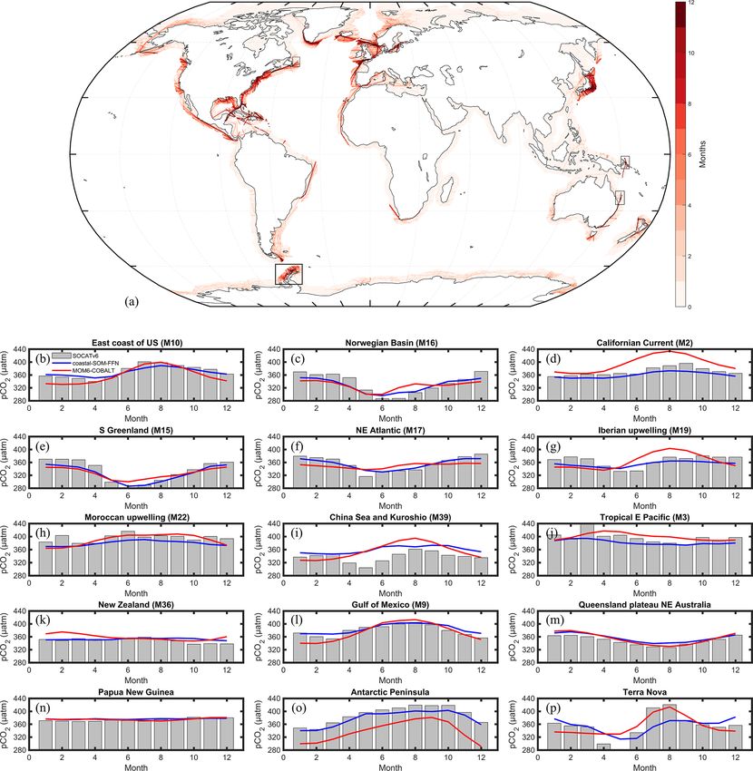
The model pCO2 seasonal evaluation against SOCATv6 seasonal MOM6-COBALT against coastal SOM-FFN eval-
is only performed in 11 MARCATS regions, namely the Cal- uation also reveals that 39 of the 45 MARCATS regions
ifornian Current (M2), tropical E Pacific (M3), the Gulf of have pCO2 seasonal amplitude biases < 20 µatm and that
Mexico (M9), the US East Coast (M10), S Greenland (M15), 34 MARCATS regions have a Pearson correlation coefficient
Norwegian Basin (M16), NE Atlantic (M17), Iberian up- > 0.5 (Table S2).
welling (M19), Moroccan upwelling (M22), China Sea and Based on this evaluation, we attribute for each MAR-
Kuroshio (M39), and New Zealand (M36). The modeled CATS region a level of confidence in the model to coastal
seasonal cycle is in good agreement with the one derived SOM-FFN agreement (“high”, “medium” and “low”; see
from SOCATv6 (Fig. 6b–l, Table S2) with absolute biases Table 1 and Fig. 1a). Out of the 45 MARCATS regions,
< 20 µatm for all of the 11 selected MARCATS and Pearson 25 are labeled with high agreement, meaning that they ful-
correlation coefficients close to 0.5 or higher except for the fill the following criteria regarding the annual mean and
Iberian Upwelling (M19, Pearson value of 0.2) and on the the seasonality (Table 1 and dotted MARCATS regions in
New Zealand shelf (M36, value of 0.3). We did not perform Fig. 1a): a bias < 20 µatm in the annual mean pCO2 between
the SOCATv6 model seasonal evaluation for the other MAR- MOM6-COBALT and coastal SOM-FFN, a bias < 20 µatm
CATS regions because the vast majority of grid cells only in the magnitude of the seasonal pCO2 cycle, and a sea-
include data for less than 4 climatological months (Fig. 6a). sonal phase characterized by a Pearson correlation coeffi-
However, we also evaluated the simulated pCO2 seasonality cient > 0.5. Note that the some MARCATS regions, i.e.,
against SOCATv6 in regions where this evaluation is not pos- the Siberian shelf (M43), the Antarctic shelf (M45), the NE
sible to be performed at the MARCATS scale. To do so, we Pacific (M1), the tropical E Atlantic (M23) and the trop-
selected four sites of smaller spatial extent than MARCATS ical W Indian Ocean(M26), also present an annual mean
for which we calculated climatological seasonal pCO2 sig- pCO2 bias < 20 µatm in the MOM6-COBALT-SOCATv6
nals from the SOCATv6 dataset and compared them with and coastal SOM-FFN-SOCATv6 comparisons (Table S1).
the model pCO2 . These sites are located off the Antarctic In addition, seven high-agreement MARCATS regions also
Peninsula, on the Queensland Plateau in NE Australia, in show a data density > 50 % (this comes to 13 MARCATS
coastal waters of Papua New Guinea and off Terra Nova in regions if we lower the data coverage to > 30 %, Fig. 1a).
Antarctica (see black boxes in Fig. 6a). In those regions, the These 7 MARCATS regions are located in contrasted coastal
absolute biases of the seasonal amplitude between MOM6- environments, i.e., three EBCs (Iberian upwelling, M19; Mo-
COBALT and SOCATv6 (Fig. 6m–p) are less than 20 µatm, roccan upwelling, M22; and the Leeuwin Current, M33),
and the phase in the seasonal cycles presents a good agree- one WBC (US East Coast, M10), one Polar region (Norwe-
ment with a Pearson correlation coefficient value of 0.8, ex- gian Basin, M16), one subpolar region (NE Atlantic, M17)
cept for the Papua New Guinea data (value of 0.5). Note and one marginal sea (Gulf of Mexico, M9). These seven
that the model SOCATv6 seasonal evaluation for Terra Nova high-agreement MARCATS regions could also result from
presents a good agreement, but the MARCATS scale (Sea the very good correspondence between the data–model an-
of Labrador, M11) evaluation to which this region belongs nual mean and seasonal patterns in environmental fields (Ta-
to reveals a low agreement, showing that a poor agreement ble S1 and Table S2, except M22, M33 and M9 for the nu-
between coastal SOM-FFN and the model does not equate trient phasing) and are therefore excellent potential candi-
to poor model skill when these regions are undersampled by dates for an analysis of the processes controlling the coastal
SOCATv6. pCO2 dynamics. A total of six additional MARCATS re-
gions fulfill the criteria related to the seasonal pCO2 eval-
3.1.3 Identifying coastal regions of high model to uation, but they fail to fulfill the annual mean pCO2 bias
coastal SOM-FFN agreement threshold of 20 µatm. These medium-agreement regions (Ta-
ble 1 and dashed regions in Fig. 1a) include two EBCs (Cal-
Overall, the pCO2 spatiotemporal analysis model–data eval- ifornian Current, M2, and SW Africa, M24), one marginal
uation shows that out of 45 MARCATS regions, 29 have an sea (Sea of Okhotsk, M41), two polar regions (Canadian
absolute bias for their annual mean < 20 µatm when MOM6- Archipelago, M13, and N Greenland, M14) and one subpolar
COBALT-coastal SOM-FFN, MOM6-COBALT-SOCATv6 region (NW Pacific, M42) shelves. The majority of marginal
and coastal SOM-FFN-SOCATv6 are compared (Table S1). seas are systematically associated with large biases relating
Together, these 29 MARCATS regions represent 65 % of the to either pCO2 or the main environmental variables. These
global coastal ocean surface area. For the 11 MARCATS re- regions fulfill only one criterion (or none of them) regard-
https://doi.org/10.5194/os-18-67-2022 Ocean Sci., 18, 67–88, 202278 A. Roobaert et al.: A framework to evaluate and elucidate the driving mechanisms of...
Figure 4. Spatial distributions of the annual mean pCO2 (µatm) generated by (a) MOM6-COBALT and (b) extracted from the SOCATv6
database, (c) model bias given as the difference between panels (a) and (b) (in µatm; red and blue colors correspond to regions in which the
pCO2 simulated by MOM6-COBALT is higher and lower than SOCATv6, respectively). (d) Spatial distribution of the annual mean pCO2
from the coastal SOM-FFN product (Laruelle et al., 2017). (e) Model bias given as the difference between panels (a) and (d).
Figure 5. Seasonal variability in ocean pCO2 (µatm). Seasonal amplitude (a) simulated by MOM6-COBALT model and (b) in the coastal
SOM-FFN product, and (c) bias between the model and coastal SOM-FFN seasonal amplitude (red indicates that simulated amplitude
exceeds coastal SOM-FFN). The seasonal amplitude is expressed as the root mean square of the monthly climatology pCO2 anomalies
(rmspCO0 , µatm). (d) Pearson correlation coefficient of the regression between the seasonal pCO2 cycles calculated by MOM6-COBALT
2
and coastal SOM-FFN. A value of 1 indicates that both signals are perfectly in phase with one another, while a value of −1 represents a
complete phase shift.
Ocean Sci., 18, 67–88, 2022 https://doi.org/10.5194/os-18-67-2022A. Roobaert et al.: A framework to evaluate and elucidate the driving mechanisms of... 79 Figure 6. (a) SOCATv6 temporal coverage evaluated as the number of months (1 to 12) where at least one pCO2 measurement is available (see details in Sect. 2). Seasonal pCO2 cycle (µatm) derived from SOCATv6 (bar in gray) and coastal SOM-FFN (in blue) and simulated by MOM6-COBALT (in red) for several MARCATS regions (b–l) and four coastal sites of smaller spatial extent than a MARCATS region (m– p). The location of the four coastal sites is represented by black boxes in panel (a). Month 1 corresponds to January. For consistency in the y axis between panels, the value of 276 µatm is not represented in panel (p) for month 5 for the SOCATv6 data. https://doi.org/10.5194/os-18-67-2022 Ocean Sci., 18, 67–88, 2022
80                                 A. Roobaert et al.: A framework to evaluate and elucidate the driving mechanisms of...

ing the pCO2 seasonality, and they are hence labeled as low-      most urgently needed, specifically those collected during pe-
agreement regions (Table 1, Fig. 1a). Other low-agreement         riods of the year that are currently not covered, to improve
regions include one EBC (Peruvian Upwelling Current, M4),         our understanding of the CO2 exchange between coastal re-
one Indian region (Bay of Bengal, M31), two tropical regions      gions and the atmosphere at the regional and global scales.
(tropical E Pacific, M3, and SE Asia, M38), two subpolar re-      In addition, only one global continuous pCO2 climatology
gions (Sea of Labrador, M11, and New Zealand, M36) and            derived by the SOM-FFN method currently exists for the
one WBC region (Brazilian Current, M6).                           coastal ocean. It would therefore be beneficial for the com-
                                                                  munity to develop other observation-based climatologies re-
3.1.4   Methodological limitations                                lying on other interpolation techniques, as is currently the
                                                                  case for the open ocean.
While our results show a relatively good agreement between           Second, the model–data comparison should also be ana-
MOM6-COBALT and coastal SOM-FFN regarding the spa-                lyzed in the light of the current limitations in the model it-
tial and temporal pCO2 distribution over the global coastal       self. OGCMs have been designed for global ocean applica-
ocean, the comparison remains challenging for several rea-        tions, and the coarse spatial resolution of these models, on
sons.                                                             the order of 0.5◦ in the present study, cannot accurately re-
   First, while the climatology of Laruelle et al. (2017,         solve mesoscale and sub-mesoscale processes and tidal mix-
coastal SOM-FFN) is currently the best available product for      ing in shelf regions even with a model configuration includ-
a model–data comparison, it has its own limitations. For in-      ing parameterizations for these processes. The coastal cur-
stance, in some regions, particularly for coastal upwellings      rents are also not always well resolved because of the coarse
such as the Moroccan (M22) and Peruvian (M4) upwellings,          resolution of the shelf bathymetry. These small-scale hydro-
the pCO2 fields generated by the coastal SOM-FFN do not           dynamic features are known to affect the spatiotemporal vari-
reproduce the high and variable pCO2 values measured in           ability of pCO2 and the air–sea CO2 exchange (Bourgeois et
situ well (see, e.g., Friederich et al., 2008; McGregor et al.,   al., 2016; Kelley et al., 1971; Lachkar et al., 2007; Laruelle
2007). Such poor performance of the coastal SOM-FFN al-           et al., 2010). Therefore, although MOM6-COBALT runs at
gorithm in these types of systems has already been identi-        0.5◦ , discrepancies between coastal SOM-FFN and MOM6-
fied by Laruelle et al. (2017). Indeed, upwelling regions are     COBALT in narrow EBCs such as the Peruvian Upwelling
still relatively poorly monitored and expand partly beyond        Current (M4) and along SW Africa (M33) could also be ex-
the coastal domain used by Laruelle et al. (2017), leading        plained by the limited spatial resolution of the model. More-
to locally skewed calibration of the SOM-FFN. Deficiencies        over, OGCMs such as MOM6-COBALT have a relatively
in the observation-based product can thus partly explain the      simple representation of biogeochemistry that does not fully
large model–data bias (106 µatm, the largest of all MAR-          capture some of the important processes of the carbon dy-
CATS regions) calculated in the Peruvian upwelling region.        namics in coastal waters, such as sea ice temporal dynam-
Moreover, although the Surface Ocean CO2 Atlas database           ics (Adcroft et al., 2019), neritic calcification (O’Mara and
(SOCAT) has expanded significantly over the past few years,       Dunne, 2019), or terrestrial and marine organic matter de-
some regions are still poorly monitored. In the coastal re-       composition and burial (Lacroix et al., 2021a, b). Moreover,
gions where no observational data exist (e.g., in the Black       the largest biases observed in marginal seas can partly be
Sea, the Sea of Okhotsk, the Bay of Bengal, Fig. 4b) in the       explained by large fluvial inputs and oceanic water flows
SOCAT database used here (SOCATv6, Bakker et al., 2016),          through fine-scale topography (e.g., straits) that are poorly
it is difficult to evaluate the performance of the SOM-FFN        represented in global OGCMs.
and thus of an Oceanic General Circulation Model (OGCM)              Finally, the annual mean and seasonal pCO2 biases be-
in reproducing the pCO2 field. In addition, for certain re-       tween the coastal SOM-FFN and MOM6-COBALT can also
gions subjected to complex dynamic biogeochemical settings        be traced back to divergences in the environmental fields sim-
(e.g., upwelling, seasonal cover of sea ice, influenced by        ulated by the model compared to observations (Tables S1 and
rivers, marginal seas), the pCO2 field reconstructed by the       S2). For instance, in most marginal seas, the model poorly re-
SOM-FFN suffers from poor performance, which can partly           solves the annual mean and seasonal cycle of SSS and nutri-
be explained by the lack of observational data. This lack         ents compared to the observations. These discrepancies im-
of observations could partly explain why MOM6-COBALT-             pact the simulated pCO2 via the controls of the SSS on the
coastal SOM-FFN pCO2 biases exceed 20 µatm in these               CO2 solubility and of nutrients on the biological pump and
regions. The seasonal model evaluation against SOCATv6            CO2 uptake. In the tropical W Atlantic (M7), which is un-
is limited at the MARCATS scale and mainly performed              der the influence of the Amazon River, the model simulates
against coastal SOM-FFN due to the very few coastal regions       lower annual mean SSS (and therefore lower pCO2 ) than the
that contain a continuous climatological seasonal pCO2 cy-        observations. In the tropical E Pacific (M3) and in South-
cle (Fig. 6a) in the SOCATv6 database. This study highlights      east Asia (M38), the poor agreement between simulated and
the regions (Fig. 1a, e.g., Indian ocean margins, the Peruvian    observed seasonal pCO2 cycle could be explained by signif-
upwelling, marginal seas) where new observational data are        icant biases in the nutrient seasonal cycles (low Pearson cor-

Ocean Sci., 18, 67–88, 2022                                                            https://doi.org/10.5194/os-18-67-2022
You can also read