Bromine from short-lived source gases in the extratropical northern hemispheric upper troposphere and lower stratosphere (UTLS)
←
→
Page content transcription
If your browser does not render page correctly, please read the page content below
Atmos. Chem. Phys., 20, 4105–4132, 2020
https://doi.org/10.5194/acp-20-4105-2020
© Author(s) 2020. This work is distributed under
the Creative Commons Attribution 4.0 License.

Bromine from short-lived source gases in the extratropical
northern hemispheric upper troposphere
and lower stratosphere (UTLS)
Timo Keber1 , Harald Bönisch1,a , Carl Hartick1,b , Marius Hauck1 , Fides Lefrancois1 , Florian Obersteiner1,a ,
Akima Ringsdorf1,c , Nils Schohl1 , Tanja Schuck1 , Ryan Hossaini2 , Phoebe Graf3 , Patrick Jöckel3 , and Andreas Engel1
1 Institute for Atmospheric and Environmental Sciences, University of Frankfurt,
Altenhöferallee 1, 60438 Frankfurt, Germany
2 Lancaster Environment Centre, Lancaster University, Lancaster, LA1 4YQ, UK
3 Institut für Physik der Atmosphäre, Deutsches Zentrum für Luft- und Raumfahrt (DLR), Oberpfaffenhofen, Germany
a now at: Karlsruhe Institute of Technology, Institute of Meteorology and Climate Research,

Hermann-von-Helmholtz-Platz 1, 76344 Eggenstein-Leopoldshafen, Germany
b now at: Research Centre Jülich, Institute for Agrosphere (IBG-3), Wilhelm-Johnen-Straße, 52428 Jülich, Germany
c now at: Atmospheric Chemistry Division, Max Planck Institute for Chemistry, Hahn-Meitner-Weg 1, 55128 Mainz, Germany

Correspondence: Timo Keber (keber@iau.uni-frankfurt.de) and Andreas Engel (an.engel@iau.uni-frankfurt.de)

Received: 4 September 2019 – Discussion started: 27 September 2019
Revised: 17 February 2020 – Accepted: 19 February 2020 – Published: 6 April 2020

Abstract. We present novel measurements of five short-              tratropical troposphere-to-stratosphere transport will result in
lived brominated source gases (CH2 Br2 , CHBr3 , CH2 ClBr,          elevated levels of organic bromine in comparison to air trans-
CHCl2 Br and CHClBr2 ). These rather short-lived gases are          ported over the tropical tropopause. The observations are
an important source of bromine to the stratosphere, where           compared to model estimates using different emission sce-
they can lead to depletion of ozone. The measurements have          narios. A scenario with emissions mainly confined to low lat-
been obtained using an in situ gas chromatography and mass          itudes cannot reproduce the observed latitudinal distributions
spectrometry (GC–MS) system on board the High Altitude              and will tend to overestimate organic bromine input through
and Long Range Research Aircraft (HALO). The instrument             the tropical tropopause from CH2 Br2 and CHBr3 . Conse-
is extremely sensitive due to the use of chemical ionization,       quently, the scenario also overestimates the amount of bromi-
allowing detection limits in the lower parts per quadrillion        nated organic gases in the stratosphere. The two scenarios
(ppq, 10−15 ) range. Data from three campaigns using HALO           with the highest overall emissions of CH2 Br2 tend to overes-
are presented, where the upper troposphere and lower strato-        timate mixing ratios at the tropical tropopause, but they are
sphere (UTLS) of the northern hemispheric mid-to-high lati-         in much better agreement with extratropical tropopause mix-
tudes were sampled during winter and during late summer to          ing ratios. This shows that not only total emissions but also
early fall. We show that an observed decrease with altitude in      latitudinal distributions in the emissions are of importance.
the stratosphere is consistent with the relative lifetimes of the   While an increase in tropopause mixing ratios with latitude
different compounds. Distributions of the five source gases         is reproduced with all emission scenarios during winter, the
and total organic bromine just below the tropopause show            simulated extratropical tropopause mixing ratios are on aver-
an increase in mixing ratio with latitude, in particular dur-       age lower than the observations during late summer to fall.
ing polar winter. This increase in mixing ratio is explained        We show that a good knowledge of the latitudinal distribu-
by increasing lifetimes at higher latitudes during winter. As       tion of tropopause mixing ratios and of the fractional con-
the mixing ratios at the extratropical tropopause are gener-        tributions of tropical and extratropical air is needed to de-
ally higher than those derived for the tropical tropopause, ex-     rive stratospheric inorganic bromine in the lowermost strato-

Published by Copernicus Publications on behalf of the European Geosciences Union.
4106                                                                 T. Keber et al.: Bromine from short-lived source gases

sphere from observations. In a sensitivity study we find max-     al., 2007; Harris et al., 2008; Dhomse et al., 2015). In the
imum differences of a factor 2 in inorganic bromine in the        lowermost stratosphere, the breakdown of VSLS provides a
lowermost stratosphere from source gas injection derived          significant bromine source in a region where (a) ozone loss
from observations and model outputs. The discrepancies de-        cycles involving bromine chemistry are known to be impor-
pend on the emission scenarios and the assumed contribu-          tant (e.g. Salawitch et al., 2005) and (b), on a per molecule
tions from different source regions. Using better emission        basis, ozone perturbations have a relatively large radiative
scenarios and reasonable assumptions on fractional contri-        effect (Hossaini et al., 2015). At present, VSLS are esti-
bution from the different source regions, the differences in      mated to supply a total of ∼ 5 (3–7) ppt (parts per trillion,
inorganic bromine from source gas injection between model         10−12 ) Br to the stratosphere, with source gas injection esti-
and observations is usually on the order of 1 ppt or less. We     mated to provide 2.2 (0.8–4.2) ppt Br and product gas injec-
conclude that a good representation of the contributions of       tion 2.7 (1.7–4.2) ppt Br (Engel and Rigby, 2018). Attribution
different source regions is required in models for a robust as-   of lower stratospheric ozone trends is complex and trends
sessment of the role of short-lived halogen source gases on       in this region are highly uncertain (Steinbrecht et al., 2017;
ozone depletion in the UTLS.                                      Ball et al., 2018; Chipperfield et al., 2018). It has been sug-
                                                                  gested that continuing negative ozone trends observed in the
                                                                  lower stratosphere (defined as about 13 to 24 km in the mid
                                                                  latitudes) may partly be related to increasing anthropogenic
1   Introduction                                                  and natural VSLS (Ball et al., 2018). While Chipperfield et
                                                                  al. (2018) suggested that the main driver for variability and
Following the detection of the ozone hole during springtime       trends in lower stratospheric ozone is dynamics rather than
over Antarctica (Farman et al., 1985) and the attribution of      chemistry, the bromine budget of the upper troposphere and
the decline in both polar and global ozone to the emissions       lower stratosphere (UTLS) needs to be well understood.
of anthropogenic halogenated compounds (see Molina and               In the past, the main focus of upper tropospheric bromine
Rowland, 1974; Solomon, 1999; Engel and Rigby, 2018),             studies for VSLS has been on the tropics, as this is the main
production and use of long-lived halogenated species, in par-     entry region for air masses to reach above 380 K potential
ticular chlorofluorocarbons (CFCs), have been regulated by        temperatures (see discussion in Engel and Rigby, 2018) and
the Montreal Protocol (WMO, 2018). This has led to de-            thus for the main part of the stratosphere. However, as many
creasing levels of chlorine in the atmosphere (Engel and          authors have shown, the lowermost stratosphere, i.e. the part
Rigby, 2018), despite recent concerns over ongoing emis-          of the stratosphere situated below 380 K but above the extrat-
sions of CFC-11, which have been attributed to unreported         ropical stratosphere, is influenced by transport from the trop-
and thus illegal production (Montzka et al., 2018; Engel          ics and from the extratropics (e.g. Holton et al., 1995; Get-
and Rigby, 2018; Rigby et al., 2019). Bromine reaching the        telman et al., 2011; Fischer et al., 2000; Hoor et al., 2005).
stratosphere has been identified as an even stronger cata-        Some authors have quantified the fraction of air in the lower-
lyst for the depletion of stratospheric ozone than chlorine       most stratosphere, which did not pass the tropical tropopause,
(Wofsy et al., 1975; Sinnhuber et al., 2009). Its relative ef-    from tracer measurements (Hoor et al., 2005; Bönisch et
ficiency on a per molecule basis is currently estimated to be     al., 2009; Ray et al., 1999; Werner et al., 2010) and oth-
60–65 times larger than that of chlorine (see discussion in       ers have used trajectory analyses to study mass fluxes and
Daniel and Velders, 2006). Long-lived bromine gases include       stratosphere–troposphere exchange (e.g. Stohl et al., 2003;
CH3 Br with partly natural and partly anthropogenic sources       Wernli and Bourqui, 2002; Škerlak et al., 2014; Appenzeller
and halons, which are of purely anthropogenic origin. Next        et al., 1996). Based on tracer measurements of mainly CO,
to long-lived gases, some chlorine and bromine from so-           Hoor et al. (2005) estimated that the fraction of air with extra-
called “very-short-lived substances” (VSLS), i.e. substances      tropical origin in the mid-latitude lowermost stratosphere of
with atmospheric lifetimes less than 6 months, can reach the      the Northern Hemisphere ranged between about 35 % during
stratosphere. It has been estimated that, for the year 2016,      winter and spring to about 55 % during summer and fall. Us-
about 25 % of the bromine entering the stratosphere is from       ing a different approach based on CO2 and SF6 observations,
VSLS (Engel and Rigby, 2018). Due to the decline in chlo-         Bönisch et al. (2009) found a similar seasonality but higher
rine and bromine from long-lived species, the relative con-       extratropical fractions, which were consistently higher than
tribution of short-lived species to stratospheric halogen load-   70 % during summer and fall and above 90 % in the entire
ing is expected to increase, which is also driven by increas-     lowermost stratosphere during October. Similarly, Bönisch
ing anthropogenic emissions of some short-lived chlorinated       et al. (2009) also derived much lower fractions of air with
halocarbons (Hossaini et al., 2017, 2019; Oram et al., 2017;      recent extratropical origin during winter and spring, which
Leedham Elvidge et al., 2015; Engel and Rigby, 2018).             were sometimes as low as 20 % during April. It has also been
   A number of factors control the abundance of ozone at mid      argued that the relative role of different source regions for the
latitudes, including influences from dynamics, chemical de-       UTLS could alter with a changing circulation (Boothe and
struction, aerosol loading and the solar cycle (e.g. Feng et      Homeyer, 2017).

Atmos. Chem. Phys., 20, 4105–4132, 2020                                            www.atmos-chem-phys.net/20/4105/2020/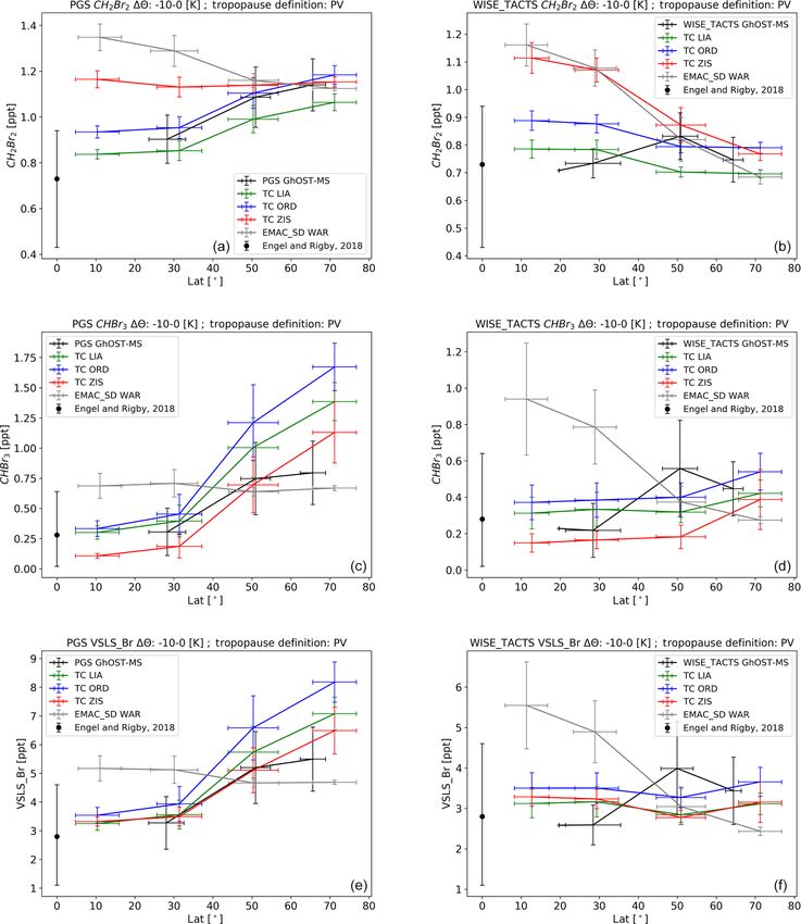
T. Keber et al.: Bromine from short-lived source gases                                                                        4107

   Both extratropical and tropical source regions are impor-        no observational evidence for this has been found (Engel and
tant for the lowermost stratosphere. A recent compilation of        Rigby, 2018). A further future increase has been suggested
entry mixing ratios of brominated VSLS to the stratosphere          (Ziska et al., 2017; Falk et al., 2017), although this projec-
(Engel and Rigby, 2018) has focused on mixing ratios rep-           tion is very uncertain and the processes associated with the
resentative of the tropical tropopause. Two pathways for in-        oceanic production of brominated VSLS are still poorly un-
put of halogens from short-lived gases are discussed. Halo-         derstood. It has also been proposed that certain source re-
gen atoms can be transported to the stratosphere in the form        gions could be more effective with respect to transport to
of the organic source gas (source gas injection (SGI)) or in        the stratosphere, in particular the Indian Ocean, the Maritime
the inorganic form as photochemical breakdown products of           Continent and the tropical western Pacific (Liang et al., 2014;
source gases (product gas injection (PGI)). Halogens from           Fernandez et al., 2014; Tegtmeier et al., 2012). The Asian
product gases are readily available for catalytic ozone deple-      monsoon has also been named as a possible pathway for
tion reactions. Source gases have to undergo a photochem-           transport of bromine from VSLS to the stratosphere (Liang
ical transformation into inorganic bromine, which can then          et al., 2014; Fiehn et al., 2017; Hossaini et al., 2016).
interact with ozone. Due to the short lifetimes of VSLS, this          While most investigations of natural VSLS focused on
release is expected to occur in the lowest part of the strato-      tropical injection of bromine to the stratosphere, this study
sphere. Therefore, brominated VSLS are particularly effec-          focuses on the extratropical bromine VSLS budget. In order
tive with respect to ozone chemistry in the lower and low-          to investigate the regional variability of bromine input into
ermost stratosphere, below about 20 km, with the associated         the lowermost stratosphere, we have performed a range of
ozone decreases exerting a significant radiative effect (Hos-       airborne measurement campaigns using an in situ gas chro-
saini et al., 2015). It has been shown that observed and mod-       matograph (GC) coupled to a mass spectrometer (MS) on
elled ozone show a better agreement if bromine from short-          board the High Altitude and Long Range Research Aircraft
lived species is included in models (Sinnhuber and Meul,            (HALO). The differences in stratospheric inorganic bromine
2015; Fernandez et al., 2017; Oman et al., 2016). In partic-        from observations and from models are discussed. In Sect. 2
ular for the Antarctic ozone hole, an enhancement in size by        we give a brief introduction to the instrument, the available
40 % and an enhancement in mass deficit by 75 % was sim-            observations and the models used for this study. Typical dis-
ulated due to VSLS (Fernandez et al., 2017) in comparison           tributions of brominated VSLS derived from these observa-
with a model run without VSLS. A delay in polar ozone re-           tions are then presented in Sect. 3 and compared to model
covery by about a decade has also been reported due to the          output from two different atmospheric models run with the
inclusion of brominated VSLS (Oman et al., 2016). In order          different emission scenarios mentioned above in Sect. 4. Fi-
to have solid projections on the effect of VSLS on ozone and        nally, in Sect. 5 the implications of the observations for inor-
climate, a good knowledge of their atmospheric distribution         ganic bromine in the stratosphere are discussed.
is thus needed for models.
   Observations indicate that the main source of brominated
VSLS is from oceans and in particular from coastal regions.         2     Observations and models
Four global emission scenarios of short-lived brominated
gases have been proposed (Warwick et al., 2006; Ordóñez             2.1    Instrumentation and observations
et al., 2012; Ziska et al., 2013; Liang et al., 2010), with vari-
ations in VSLS source strengths of more than a factor of 2          The data presented here have been measured with the in situ
between them (Engel and Rigby, 2018). In the past, these            Gas chromatograph for Observational Studies using Trac-
scenarios have been compared to each other and to obser-            ers – Mass Spectrometer (GhOST-MS) deployed on board
vations; large differences have been identified in modelled         HALO. GhOST-MS is a two-channel GC instrument. An
tropospheric mixing ratios of CHBr3 and CH2 Br2 , along             electron capture detector (ECD) is used in an isothermal
with estimates of stratospheric bromine input (Hossaini et          channel in a similar set-up as used during the SPURT cam-
al., 2013, 2016; Sinnhuber and Meul, 2015). Hossaini et             paign (Bönisch et al., 2009, 2008; Engel et al., 2006) to
al. (2013) concluded that the lowest suggested emissions of         measure SF6 and CFC-12 with a time resolution of 1 min.
CHBr3 (Ziska et al., 2013) and the lowest suggested emis-           The second channel is temperature programmed and uses a
sions of CH2 Br2 (Liang et al., 2014) yielded the overall best      cryogenic pre-concentration system (Obersteiner et al., 2016;
agreement in the tropics and thus the most realistic input          Sala et al., 2014) and a mass spectrometer (MS) for detection.
of stratospheric bromine from VSLS. They also concluded             It is similar to the set-up described by Sala et al. (2014) and
that “Averaged globally, the best agreement between mod-            measures halocarbons in the chemical ionization mode (e.g.
elled CHBr3 and CH2 Br2 with long-term surface observa-             Worton et al., 2008) with a time resolution of 4 min. As ex-
tions made by NOAA/ESRL is obtained using the top-down              plained in Sala et al. (2014), CH2 BrCl2 and CH2 Br2 are not
emissions proposed by Liang et al. (2010)”. It has also been        separated chromatographically during normal measurements
proposed that VSLS emissions may have increased by 6 %–             with GhOST-MS, as this would require too much time. In-
8 % between 1979 and 2013 (Ziska et al., 2017), although            stead, a correlation between the two species from either in-

www.atmos-chem-phys.net/20/4105/2020/                                                Atmos. Chem. Phys., 20, 4105–4132, 2020
4108                                                                 T. Keber et al.: Bromine from short-lived source gases

dependent measurements or measurements of the two species         separately in Fig. S1 in the Supplement. For this combined
from dedicated flights are used. Such dedicated flights have      dataset, some observations from the TACTS campaign have
been performed during the WISE and PGS campaigns (de-             been omitted, where some extremely high values of VSLS
fined below). The procedure of how CHBrCl2 and CH2 Br2            (up to a factor of 10 above typical tropospheric mixing ra-
are derived from the single chromatographic peak with this        tios) were observed in the UTLS, which are suspected of be-
additional information is explained in Sala et al. (2014).        ing contaminated. The source of the contamination is, how-
While CH4 has been used as chemical ionization gas for the        ever, unknown. Figure 3 shows an example time series of
TACTS campaign (defined below) and for the tropical mea-          halon 1301 (CF3 Br), CH2 Br2 and CHBr3 , ozone and mean
surements discussed in Sala et al. (2014), a change in chemi-     age of air calculated from the SF6 measurements obtained
cal ionization gas was necessary for later measurements due       during a typical flight in the Arctic in January 2016. It is
to safety reasons. During the PGS campaign pure Argon was         clearly visible that the halocarbons are correlated amongst
used, which resulted in very good sensitivities but also an in-   each other, whereas they are anticorrelated with ozone and
terference with water vapour. In order to avoid this interfer-    mean age. It is further evident from Fig. 3 that the shortest-
ence for the mid-latitude (more humid) measurements dur-          lived halocarbon measured by GhOST-MS, i.e. CHBr3 , de-
ing WISE, a mixture of Argon and methane (non-burnable,           creases much faster with increasing ozone than the longer-
below 5 % methane) was used as ionization gas. These (and         lived CH2 Br2 or the long- lived source gas halon 1301. Note
some other) changes resulted in different performances of the     that the local lifetimes of the halocarbons may differ signifi-
instrument during different campaigns. Typical performance        cantly from their typical mid-latitude lifetimes shown in Ta-
details of the instrument are given for the WISE and PGS          ble 1. Lifetimes generally increase with (a) decreasing tem-
campaigns in Table 1 for the brominated hydrocarbons.             perature for species with a sink through the reaction with
   The instrument is tested for non-linearities, memory and       the OH radical and (b) with decreasing solar irradiation for
blank signals, which are corrected where necessary (see the       species with direct photolytic sink. Therefore, in particular
description in Sala, 2014, and Sala et al., 2014, for details).   during winter, lifetimes are estimated to increase consider-
Table 1 also includes typical local lifetimes of the differ-      ably with increasing latitude due to the decreased solar illu-
ent VSLS species and the global lifetimes of the long-lived       mination and low temperatures.
species. The instrument was deployed during several cam-
paigns of the German research aircraft HALO, providing ob-        2.2   Models and meteorological data
servations in the UTLS over a wide range of latitudes and
different seasons mainly in the Northern Hemisphere. Some         Data from two different models were used in this study:
observations from the Southern Hemisphere are also avail-         ESCiMo (Earth System Chemistry Integrated Modelling)
able, but, due to their sparsity, they will not be part of this   data from the EMAC (ECHAM/MESSy Atmospheric Chem-
work.                                                             istry) chemistry climate model (CCM) and the TOMCAT
   GhOST-MS measurements from three HALO missions                 (Toulouse Off-line Model of Chemistry And Transport)
will be presented and discussed here. The first atmospheric       chemistry transport model (CTM).
science mission of HALO was TACTS (Transport and Com-                For EMAC data, we used results from the simulations in
position in the Upper Troposphere/Lowermost Stratosphere),        the so-called specified dynamics (SD) mode, for which the
conducted between August and September 2012, with a fo-           model was nudged (by Newtonian relaxation) towards ERA-
cus on the Atlantic sector of the mid latitudes of the Northern   Interim meteorological reanalysis data from the European
Hemisphere. The second campaign was PGS, a mission con-           Centre for Medium-Range Weather Forecasts (ECMWF;
sisting of three sub-missions: POLSTRACC (Polar Strato-           Dee et al., 2011). T42 spectral model resolution was used,
sphere in a Changing Climate), GW-LCYCLE (Investiga-              corresponding to a quadratic Gaussian grid of approximately
tion of the Life cycle of gravity waves) and SALSA (Sea-          2.8◦ by 2.8◦ horizontal resolution, and the vertical resolution
sonality of Air mass transport and origin in the Lowermost        comprised 90 hybrid sigma-pressure levels up to 0.01 hPa.
Stratosphere). PGS took place mainly in the Arctic between        The model output has been subsequently interpolated to pres-
December 2015 and March 2016. Finally, the GhOST-MS               sure levels between 1000 and 0.01 hPa. The emissions of
was deployed during the WISE (Wave-driven ISentropic Ex-          VSLS were taken from the emission scenario 5 in Warwick
change) mission between September and October 2017. The           et al. (2006). The EMAC SD simulations with 90 vertical
dates of the missions and some parameters on the available        levels, as described in detail by Jöckel et al. (2016), were in-
observations are summarized in Table 2, and the flight tracks     tegrated with an internal model time step length of 12 min,
are shown in Figs. 1 and 2. As the WISE and TACTS cam-            and the data have been output every 10 h from which the
paigns covered a similar time of the year and latitude range,     monthly averages on pressure levels have been derived. The
the data from the two campaigns have been combined into           SC1SD-base-01 simulation, which has been used here, has
a single dataset, which we will refer to as “WISE_TACTS”.         been branched off from RC1SD-base-10 (see Jöckel et al.,
Vertical profiles of the two major bromine VSLS, CH2 Br2          2016) at 1 January 2000 using the RCP8.5 emissions and
and CHBr3 , for the TACTS and WISE campaigns are shown            greenhouse gas scenario.

Atmos. Chem. Phys., 20, 4105–4132, 2020                                            www.atmos-chem-phys.net/20/4105/2020/
T. Keber et al.: Bromine from short-lived source gases                                                                                                            4109

Table 1. Brominated species measured with Gas chromatograph for Observational Studies using Tracers – Mass Spectrometer (GhOST-
MS) during three High Altitude and Long Range Research Aircraft campaigns, described in Table 2. Tropospheric mole fractions (parts per
trillion, ppt; 10−12 ) of the halons are taken from Table 1-1 in Engel and Rigby (2018) and from Table 1-7 for the bromocarbons (marine
boundary layer value mixing ratios). Lifetimes of bromocarbons are local lifetimes for upper tropospheric conditions (10 km altitude, 25–
60◦ N) from Table 1-5 in Carpenter and Reimann (2014) and global/stratospheric lifetimes are from Table A-1 in WMO 2018 (Burkholder,
2018). Local lifetimes are given in days (d), while global and stratospheric lifetimes are given in years (yr). Reproducibilities and detection
limits of GhOST have been determined during the WISE and the PGS campaigns. For the TACTS campaign instrument, performance was
similar to that reported in Sala et al. (2014).

                                                                                  GhOST-MS characteristics                        Typical lifetime
        Name                             Formula              Troposph.          Reprod.          Decetion limit        Fall    Winter       Global      Strat.
                                                                               PGS WISE           PGS WISE
                                                                     (ppt)      (%)        (%)    (ppq)      (ppq)       (d)         (d)        (yr)       (yr)
        Halon 1301                       CF3 Br                      3.36        0.4          1       7         50       n/a         n/a          72      73.5
        Halon 1211                       CBrClF2                     3.59        0.2        0.5       2          6       n/a         n/a          16       41
        Halon 1202                       CBr2 F2                    0.014        2.8        7.6       1          6       n/a         n/a         2.5       36
        Halon 2402                       CBrF2 CBrF2                 0.41        0.6        1.5       2          7       n/a         n/a          28       41
        Dibromomethane                   CH2 Br2                      0.9        0.2        0.7       3         11      405         890          n/a       n/a
        Tribromomethane                  CHBr3                        1.2        0.6        2.2       9         85       44          88          n/a       n/a
        Bromochloromethane               CH2 BrCl                      0.1       2.3        9.2      20        130      470        1050          n/a       n/a
        Dichlorobromomethane             CHBrCl2                      0.3        0.8        3.4       3          2      124         250          n/a       n/a
        Dibromochloromethane             CHBr2 Cl                     0.3        0.7        2.2       4          2       85         182          n/a       n/a

      n/a: not applicable.

Table 2. Brief description of measurement campaigns with the High Altitude and Long Range Research Aircraft (HALO) used for this study.

  Name                                       Time period                      Campaign base                           Brief description
  TACTS: Transport and Com-                  late August 2012–                Oberpfaffenhofen, Germany,              Covers changes in UTLS chemical
  position in the Upper Tropo-               September 2012                   and Sal, Cabo Verde                     composition during the transition from
  sphere/Lowermost Stratosphere                                                                                       summer to fall
  WISE: Wave-driven ISentropic               September–                       Shannon, Ireland                        Study on troposphere–stratosphere
  Exchange                                   October 2017                                                             exchange in mid latitudes
  PGS, POLSTRACC,                            December 2015–                   Kiruna, Sweden                          Study the polar UTLS during winter, in-
  GW-LCYCLE, SALSA∗                          March 2016                                                               cluding the effect of chemical ozone de-
                                                                                                                      pletion.
∗ PGS is a synthesis of three measurement campaigns: POLSTRACC (The Polar Stratosphere in a Changing Climate), GW-LCYCLE (Investigation of the Life cycle of gravity
waves) and SALSA (Seasonality of Air mass transport and origin in the Lowermost Stratosphere).

   The TOMCAT model (Chipperfield, 2006; Monks et al.,                                   CH2 Br2 , CH2 BrCl, CHBr2 Cl and CHBrCl2 ) are calculated
2017) is driven by analysed wind and temperature fields                                  using the relevant kinetic data from Burkholder et al. (2015).
taken 6-hourly from the ECMWF ERA-Interim product.                                          Local tropopause information for the flights with HALO
Here, the model was run with T42 horizontal resolution (2.8◦                             have been derived from ERA-Interim data. The climatolog-
by 2.8◦ ) and with 60 vertical levels, extending from the sur-                           ical tropopause has been calculated based on potential vor-
face to ∼ 60 km. The internal model time step was 30 min,                                ticity (PV) according to the method described in Škerlak et
and tracers were output as monthly means. This configura-                                al. (2015) and Sprenger et al. (2017) based on the ERA-
tion of the model has been used in a number of VSLS-related                              Interim reanalysis. As the PV tropopause is not physically
studies and is described by Hossaini et al. (2019). In this                              meaningful in the tropics, the level with a potential temper-
study, three different VSLS emission scenarios are used with                             ature of 380 K has been adapted for the tropopause where
TOMCAT (Liang et al., 2010; Ordóñez et al., 2012; Ziska et                               the 2 PVU (potential vorticity unit) level is located above the
al., 2013). In the case of the Liang et al. (2010) scenario, their                       380 K level.
scenario A has been used. Chemical breakdown by reaction
with OH and photolysis in the model for all VSLS (CHBr3 ,

www.atmos-chem-phys.net/20/4105/2020/                                                                        Atmos. Chem. Phys., 20, 4105–4132, 2020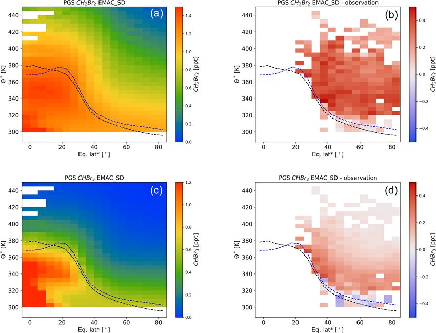
4110 T. Keber et al.: Bromine from short-lived source gases
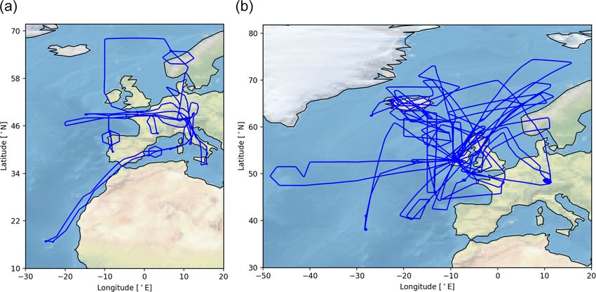
Figure 1. Flight tracks of HALO during the (a) TACTS campaign (late August and September 2012) and (b) WISE campaign (September–
October 2017). The basis of the TACTS campaign was mainly Oberpfaffenhofen (near Munich in Germany), while the basis of the WISE
campaign was Shannon (Ireland).
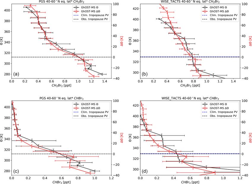
bins. In the vertical direction, three different coordinates are
used in this paper. These are potential temperature θ , poten-
tial temperature above the local tropopause 1 θ and finally a
coordinate we refer to as θ ∗ , which is calculated by adding
the potential temperature of the mean tropopause to 1 θ. We
used the dynamical tropopause, defined by a potential vor-
ticity of 2 PVU or by a potential temperature of 380 K in the
tropics (see Sect. 2), as a reference surface.
3.1 Mean vertical profiles
All measurements from the individual campaigns have been
binned into 10 K potential temperature bins between −40
Figure 2. Flight tracks of HALO during the PGS campaign (De- and 100 K of 1θ . For potential temperature binning, the 10 K
cember 2015 to April 2016). The basis of the campaign was mainly
bins have been chosen ranging from 40 K below the mean
Kiruna in northern Sweden.
tropopause to 100 K above the mean tropopause. In this way,
the centres of the 1θ and θ bins are the same relative to the
mean tropopause observed during the measurements. The re-
3 Observed distribution and atmospheric gradients of sults are presented for the two main VSLS bromine source
different brominated VSLS gases CH2 Br2 and CHBr3 , averaged over equivalent latitude∗
of 40–60◦ N in Fig. 4 for PGS (northern hemispheric win-
Spatial distributions are shown in tropopause-relative coor- ter) and the WISE_TACTS combined dataset (late summer
dinates and as functions of equivalent latitude. As equiva- to fall, Northern Hemisphere). Results for the minor VSLS
lent latitude is mainly a useful horizontal coordinate for the and total organic bromine are shown in Figs. S2 and S3.
stratosphere, we chose to use standard latitude for all mea- Only bins which contain at least five data points have been
surements below the tropopause and equivalent latitude for included in the analysis. The results are also summarized in
all measurements above the tropopause. We refer to this co- Tables 3 and 4 for the same latitude intervals for all species
ordinate as equivalent latitude∗ . As the observations typically and for total organic bromine derived from the five bromi-
cover a range of latitudes, vertical profiles are shown for 20◦ nated VSLS. The tropopause mole fractions shown in Ta-
Atmos. Chem. Phys., 20, 4105–4132, 2020 www.atmos-chem-phys.net/20/4105/2020/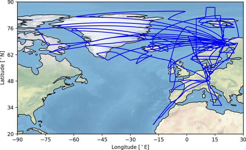
T. Keber et al.: Bromine from short-lived source gases                                                                       4111

bles 3 and 4 have been derived as the average of all values in    variability averaged over the four lowest stratospheric bins
that latitude interval and within 10 K below the tropopause.      when using 1θ was always lower than in the four lowest bins
The potential temperature of the average tropopause has been      above the climatological tropopause using θ as a coordinate
used for θ averaging, while the potential temperature dif-        (see Tables 3 and 4). This shows that using the tropopause-
ference to the local tropopause has been used as reference        centred coordinate system 1θ reduces the variability in the
when averaging in 1θ coordinates. Due to this different sam-      stratosphere, and it is therefore the best suited coordinate sys-
pling, a higher range in 1θ is achieved than in θ , as the        tem to derive typical distributions. In the troposphere, the
actual tropopause altitude varies. We have checked the va-        variability is larger when using 1θ coordinates than for θ ,
lidity of using means to represent the data, by comparing         indicating that the variability in the free troposphere is not
means and medians. Differences were always below 5 % of           influenced by the potential temperature of the tropopause.
the mean tropopause mixing ratios. We have thus chosen to         The observed variabilities were found to be very similar for
use means throughout this paper. The uncertainties given in       the WMO and PV tropopause definitions (not shown). As the
all figures are 1σ standard deviations of these means, both for   dynamical PV tropopause is generally expected to be better
the vertical and horizontal error bars. In the WISE_TACTS         suited for tracer studies, we decided to reference all data to
dataset, total organic bromine at the dynamical tropopause        the dynamical tropopause.
between 40 and 60◦ N was 4.05 and 3.5 ppt, using 1θ and
θ as vertical coordinates, respectively. Higher mixing ratios     3.2   Latitude–altitude cross sections
of total organic bromine were found during the winter cam-
paign PGS, when average tropopause mixing ratios were 5.2         We slightly diverge from the coordinate system used to
and 4.9 ppt both using 1θ and θ as vertical coordinates.          present zonal mean latitude–altitude distributions used in
These mixing ratios are considerably higher than the tropical     previous work (e.g. Bönisch et al., 2011; Engel et al., 2006),
tropopause values of organic bromine derived in the vicinity      where equivalent latitude and potential temperature were
of the tropical tropopause (Engel and Rigby, 2018) as will be     used as horizontal and vertical coordinates. We use equiv-
discussed in detail below. When using the WMO definition          alent latitude∗ as a horizontal coordinate, i.e. latitude for all
of the tropopause, the total organic bromine at mid latitudes     tropospheric observations and equivalent latitude for obser-
was lower by up to 0.5 ppt than using the PV tropopause, re-      vations at or above the tropopause. As a vertical coordinate
flecting the fact that the WMO tropopause is usually slightly     we have chosen to use a modified potential temperature co-
higher than the dynamical tropopause using the 2 PVU defi-        ordinate θ ∗ (see explanation above, Sect. 3). In this way,
nition (e.g. Gettelman et al., 2011).                             all measurements are presented relative to a climatological
   CHBr3 showed the largest vertical gradients of all species     tropopause, which has been derived from ERA-Interim re-
discussed here, followed by CHBr2 Cl. This is well in line        analysis as zonal mean for the latitude of interest and the
with their atmospheric lifetimes (see Table 1), which will        specific months of the campaign (see Sect. 2 for campaign
generally decrease with an increase in bromine atoms in the       details). This is expected to reduce variability by applying
molecule and is shortest for CHBr3 , followed by CHBr2 Cl.        the information from 1θ , yet the absolute vertical informa-
The relationship between lifetime and vertical gradient is less   tion is also maintained. In order to ensure that this tropopause
clear for the longer-lived species, where vertical profiles are   value is representative also of the period of our observa-
expected to be more influenced by transport. In particular, the   tions, we compare the potential temperature of the campaign-
vertical gradient of CHBrCl2 is closer to the vertical gradi-     based tropopause with the climatological tropopause. The
ent of CH2 Br2 than to that of CHBr2 Cl, although the lifetime    campaign-based tropopause has been calculated by averag-
should be closer to CHBr2 Cl. This could be related to the        ing the tropopause at all locations for which observations
way that CHBrCl2 is derived, as it is not chromatographi-         are available during the campaign. For the latitude band be-
cally separated from CH2Br2 (see Sect. 2.1 and Sala et al.,       tween 40 and 60◦ N, the climatological PV tropopause for
2014). The strongest vertical gradients with respect to both      the TACTS_WISE time period was derived to be at 329 K,
θ and 1θ were observed during the winter campaign PGS,            in excellent agreement with the campaign-based tropopause,
with the exception of CHBr3 , which was nearly completely         which was also at 329 K. For the PGS campaign, both the cli-
depleted for all campaigns at 40 K above the tropopause and       matological tropopause and the campaign-based tropopause
thus shows very similar averaged gradients over this poten-       were found to be at 312 K. In contrast to the campaign-based
tial temperature region. When evaluated only for the first        tropopause, the climatological tropopause is also available
20 K above the tropopause, the gradient of CHBr3 was also         for latitude bands and longitudes not covered by our obser-
much larger during PGS then during WISE and TACTS. The            vations and will be more representative of typical conditions
short lifetime and strong vertical gradient of CHBr3 is also      during the respective season and latitude.
reflected in the largest relative variability (see Tables 3 and      Figure 5 shows the distributions of the two main VSLS
4).                                                               bromine source gases, CH2 Br2 and CHBr3 , in the coordi-
   We further determined the variability of the different         nate system discussed above for the two campaign seasons
species in 10 K intervals of θ and 1θ . For all campaigns, the    (PGS: winter; WISE_TACTS: late summer to early fall). The

www.atmos-chem-phys.net/20/4105/2020/                                              Atmos. Chem. Phys., 20, 4105–4132, 2020
4112                                                                              T. Keber et al.: Bromine from short-lived source gases

Table 3. Averaged mole fractions (parts per trillion, ppt; 10−12 ) and vertical gradients of brominated very-short-lived substances from the
combined WISE and TACTS dataset, representative of 40–60◦ N during late summer to early fall (data from late August to October). Data
have been averaged using potential temperature, θ , and potential temperature difference to the tropopause, 1θ, as vertical profile coordinates.
Tropopause (TP) mixing ratios are from the 10 K bin below the dynamical tropopause (see text for details). The 10 K bin standard deviations
in the table represent the variability averaged over the four lowest stratospheric bins. The average potential temperature of the tropopause
during the WISE and TACTS campaigns has been calculated from the European Centre for Medium-Range Weather Forecasts data at the
locations of our measurements.

                                                     θ                                                               1θ
 WISE and TACTS           Mole fraction (ppt)            Gradient         10 K bin σ         Mole fraction (ppt)          Gradient         10 K bin σ
                                                                    (TP − TP + 40 K)                                                 (TP − TP + 40 K)
                             TP    TP + (30–40 K)        (% K−1 )              (ppt)            TP    TP + (30–40 K)      (% K−1 )                 (ppt)
 CH2 Br2             0.79 ± 0.07       0.67 ± 0.15           0.39               0.12    0.83 ± 0.08       0.59 ± 0.09         0.74                 0.09
 CHBr3               0.45 ± 0.18       0.26 ± 0.28           1.08               0.20    0.56 ± 0.26       0.11 ± 0.05         1.99                 0.11
 CH2 BrCl             0.18 ± 0.1       0.17 ± 0.08           0.08                0.1    0.23 ± 0.11       0.15 ± 0.07          0.8                  0.1
 CHBrCl2             0.16 ± 0.03       0.13 ± 0.03           0.48               0.03    0.16 ± 0.02       0.12 ± 0.02         0.73                 0.02
 CHBr2 Cl            0.12 ± 0.03       0.09 ± 0.04           0.74               0.04    0.13 ± 0.03       0.06 ± 0.02         1.28                 0.03
 Total Br            3.52 ± 0.73       2.48 ± 1.18           0.73               0.83    3.99 ± 1.15       1.89 ± 0.42         1.31                 0.50

Table 4. Averaged mole fractions and vertical gradients of brominated VSLS during the PGS campaign. Data have been averaged using
potential temperature, θ, and potential temperature difference to the tropopause, 1θ, as vertical profile coordinates. Tropopause (TP) mixing
ratios are from the 10 K bin below the dynamical tropopause (see text for details). The 10 K bin standard deviations in the table represent the
variability averaged over the four lowest stratospheric bins. The average potential temperature of the tropopause during the PGS campaign
has been calculated from ECMWF data at the locations of our measurements.

                                                 θ                                                                 1θ
       PGS                Mole fraction (ppt)              Gradient    10 K bin σ          Mole fraction (ppt)          Gradient     10 K bin σ
                             TP    TP + (30–40 K)          (% K−1 )          (ppt)              TP      TP + 40 K       (% K−1 )           (ppt)
       CH2 Br2      1.08 ± 0.08         0.50 ± 0.09             1.34          0.18      1.09 ± 0.13    0.53 ± 0.09           1.28          0.11
       CHBr3        0.66 ± 0.12         0.07 ± 0.04             2.22          0.26       0.75 ± 0.3    0.07 ± 0.03           2.26          0.13
       CH2 BrCl     0.25 ± 0.03         0.13 ± 0.02             1.16          0.05      0.26 ± 0.05    0.14 ± 0.02           1.14          0.03
       CHBrCl2      0.20 ± 0.01         0.09 ± 0.02             1.35          0.03      0.20 ± 0.02    0.10 ± 0.02           1.29          0.02
       CHBr2 Cl     0.16 ± 0.02         0.04 ± 0.01             1.89          0.04      0.16 ± 0.04    0.04 ± 0.01           1.86          0.03
       Total Br     4.91 ± 0.54         1.53 ± 0.34             1.72          1.28      5.20 ± 1.25    1.60 ± 0.33           1.73          0.70

data have been binned in 5◦ latitude and 5 K intervals of the                 from VSLS has been converted to inorganic bromine. This
modified potential temperature coordinate θ ∗ . As expected,                  stratospheric character is in agreement with the observation
the distributions closely follow the tropopause (indicated by                 of air masses with very high mean age of air derived from
the dashed line), with mixing ratios decreasing with distance                 SF6 observations of GhOST-MS (see Fig. 3), reaching up to
to the tropopause and also with increasing equivalent lati-                   5 years for the oldest air (not shown). This is air which has
tude. The distributions observed during the WISE and the                      descended inside the polar vortex and has not been in contact
TACTS campaigns show rather high levels of CH2 Br2 in the                     with tropospheric sources for a long time, allowing even the
lower stratosphere, with a depletion of only about 35 % at                    longer-lived CH2 Br2 to be nearly completely depleted.
40–50 K above the tropopause. This is consistent with the
rather long lifetime of CH2 Br2 in the cold upper troposphere                 3.3      Upper tropospheric latitudinal gradients
and lower stratosphere (Hossaini et al., 2010). The shorter-
lived CHBr3 is depleted by about 85 % already at 20–30 K                      If air is transported into the lowermost stratosphere via ex-
above the tropopause during the winter campaign PGS. In                       change with the extratropical upper troposphere, the lev-
the case of the winter campaign PGS, mixing ratios close                      els of organic bromine compounds are likely to be differ-
to zero at the highest flight altitudes are also observed for                 ent than for air being transported into the stratosphere via
the longer-lived CH2 Br2 , indicating that in the most strato-                the tropical tropopause. In order to investigate the variability
spheric air masses observed during PGS nearly all bromine                     and the gradient in the upper tropospheric input region, we
                                                                              binned our data according to latitude and to potential tem-

Atmos. Chem. Phys., 20, 4105–4132, 2020                                                           www.atmos-chem-phys.net/20/4105/2020/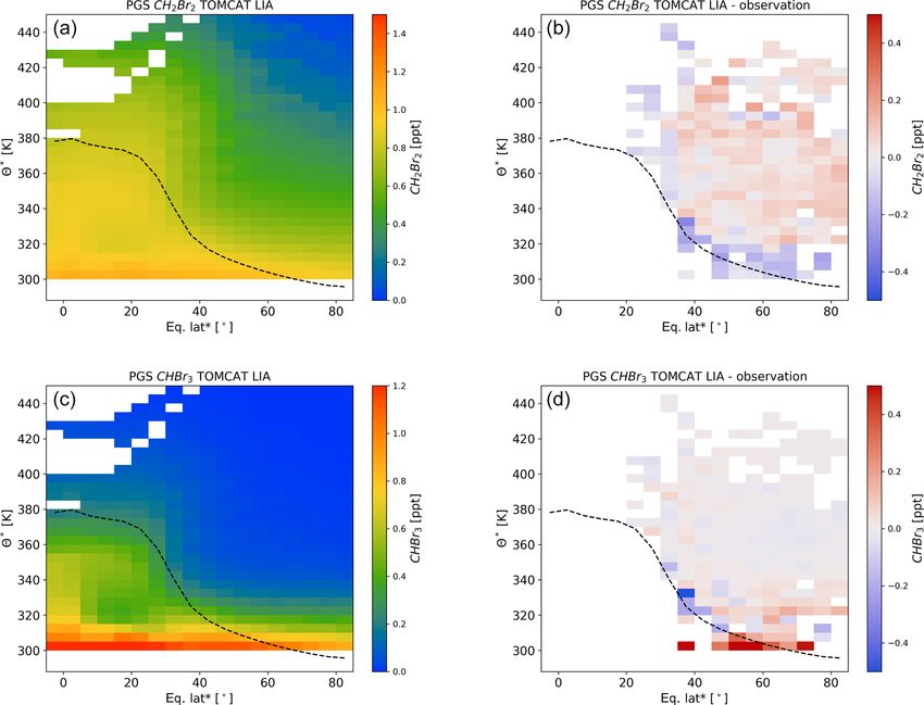
T. Keber et al.: Bromine from short-lived source gases                                                                                4113

Figure 3. Example of data gathered during a single flight of HALO during the PGS campaign. The flight PGS 12 started on 31 January 2016
from Kiruna in northern Sweden. Panel (a) shows measurements of the long-lived brominated source gas halon 1301 (CF3 Br) and the short-
lived source gases CH2 Br2 and CHBr3 , all measured with the GhOST-MS. Panel (b) shows flight altitude, ozone (parts per billion, ppb;
10−9 ; measured by the FAIRO instrument; Zahn et al., 2012) and mean age of air derived from SF6 measurements from the ECD channel
of the GhOST-MS (1 min time resolution; see Bönisch et al., 2009, for a description of the measurement technique). An air mass with low
ozone and also low mean age of air was observed during the middle of the flight between about 10:00 and 11:00 UTC. High mixing ratios
of all three source gases are found in this region, as well as during take-off and landing of the aircraft. CHBr3 mixing ratios are close to
detection limit when flying in aged stratospheric air masses, indicating a complete conversion of the bromine to its inorganic form.

perature difference to the tropopause. All data in a range of           increase with latitude is observed from 3.3 ppt around 30◦ N
10 K below the local dynamical tropopause have been aver-               (20–40◦ N equivalent latitude∗ ) via 3.8 ppt around 50◦ N
aged to characterize the upper tropospheric input region. For           (40–60◦ N equivalent latitude∗ ) to 5.5 ppt in the high lat-
these upper tropospheric data, standard latitude has been cho-          itudes (60–80◦ N equivalent latitude∗ ). There is consider-
sen and not equivalent latitude as for the stratospheric data.          able variability in these values derived in the upper tropo-
The latitudinal gradients are shown in Fig. 6 for CH2 Br2 ,             sphere, due to the short lifetime of these compounds and
CHBr3 and total organic bromine derived from the sum of all             the high variability in emissions depending on the source re-
VSLS (including the mixed bromochlorocarbons CH2 BrCl,                  gion. Nevertheless, there is a clear tendency for an increase
CHBrCl2 and CHBr2 Cl), each weighted by the number of                   in tropopause mixing ratios with latitude, particularly during
bromine atoms. For the tropical tropopause, input mixing                northern hemispheric winter. This is most probably related
ratios from different measurement campaigns have recently               to the increase in lifetime with latitude, as especially during
been reviewed by Engel and Rigby (2018). They found that                the wintertime PGS campaign the photolytical breakdown in
total organic bromine from these five compounds averaged                higher latitudes is slower than in lower latitudes. Additional
between 375 and 385 K; i.e. around the tropical tropopause              effects due to the sources and their latitudinal, seasonal and
it was 2.2 (0.8–4.2) ppt and in the upper tropical tropopause           regional variability cannot be excluded. However, we note
layer (TTL) (365–375 K potential temperature) it was around             that emissions are most likely to be largest during summer,
2.8 (1.2–4.6) ppt. These upper TTL mixing ratios have also              as shown in Hossaini et al. (2013), which would not explain
been included as reference in Fig. 6 (see also Table 5). The            the large mixing ratios of brominated VSLS in the upper tro-
average mixing ratios derived here for the 10 K interval be-            posphere in high latitudes during winter.
low the extratropical tropopause are larger. For data in the
late summer to early fall from TACTS and WISE (Table 3),
they increase from 2.6 ppt around 30◦ N (20–40◦ N equiva-               4   Comparison with model-derived distributions
lent latitude∗ ) to 3.8 ppt around 50◦ N (40–60◦ N equivalent
                                                                        As bromocarbons are an important source of stratospheric
latitude∗ ), while no further increase is found for higher lat-
                                                                        bromine, it is worthwhile to investigate if current models can
itudes with a total organic bromine mixing ratio of 3.4 ppt.
                                                                        reproduce the observed distributions shown in Sect. 3. This
For the winter measurements during PGS (Table 4), a clear
                                                                        is a prerequisite to realistically simulate the input of bromine

www.atmos-chem-phys.net/20/4105/2020/                                                      Atmos. Chem. Phys., 20, 4105–4132, 2020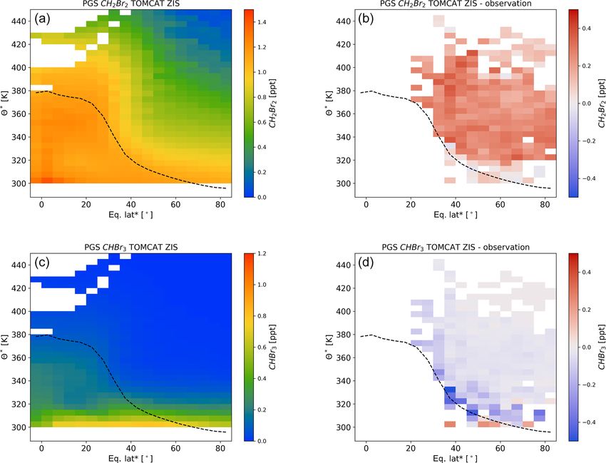
4114 T. Keber et al.: Bromine from short-lived source gases
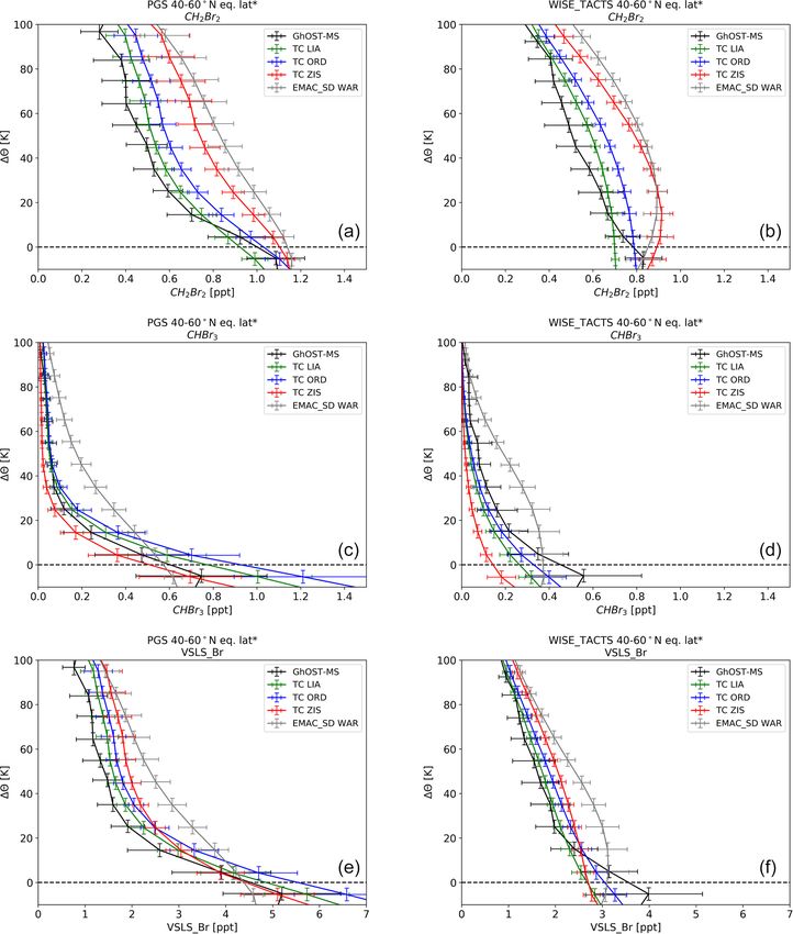
Figure 4. Vertical profiles of CH2 Br2 (a, b) and CHBr3 (c, d) averaged over 40–60◦ of equivalent latitude∗ and all flights during the PGS
campaign (a, c, late December 2015 to March 2016) and from the merged dataset from the TACTS and WISE campaigns (b, d, representative
of late summer to fall). The data are displayed as a function of potential temperature and potential temperature above the tropopause. The
dashed blue line shows the zonal mean dynamical tropopause derived from ERA-Interim during September and October of the respective
years in the Northern Hemisphere between 40 and 60◦ latitude, while the dashed black line is the average dynamical tropopause derived for
the times and locations of our observations. Both vertical and horizontal error bars denote 1σ variability.
ex-trop
Table 5. Mixing ratios of organic VSLS bromine in air at the tropical, and respectively extratropical (40–60◦ N), tropopause (Brorg
trop
and Brorg ) used in the calculation of inorganic bromine (Bry ) for the observation (OBS), and respectively the models, using the emission
scenarios of Liang et al. (2010), Ordóñez et al. (2012), Ziska et al. (2013) and Warwick et al. (2006). For the Warwick et al. (2006) scenario,
the data have been derived from the EMAC model, while for the other scenarios the TOMCAT model has been used. For the tropics, annual
average for the years 2012 to 2016 have been calculated between 10◦ N and 10◦ S in a potential temperature range from 365 to 375 K. The
tropical mixing ratios for the observations are from the observations compiled in the 2018 WMO report (Engel and Rigby, 2018) in the
tropics between 365 and 375 K potential temperature. All data presented are shown in parts per trillion.
Tropics Extratropics WISE and TATS Extratropics PGS
CH2 Br2 CHBr3 TOT CH2 Br2 CHBr3 TOT CH2 Br2 CHBr3 TOT
OBS 0.73 0.28 2.80 0.83 0.56 3.99 1.09 0.75 5.20
LIANG 0.82 0.26 3.06 0.70 0.32 2.84 0.99 1.00 5.73
ORDONEZ 0.91 0.28 3.30 0.79 0.44 3.27 1.10 1.21 6.58
ZISKA 1.13 0.10 3.18 0.87 0.18 2.77 1.13 0.69 5.10
WARWICK 1.28 0.84 5.48 0.83 0.37 3.07 1.16 0.62 4.59
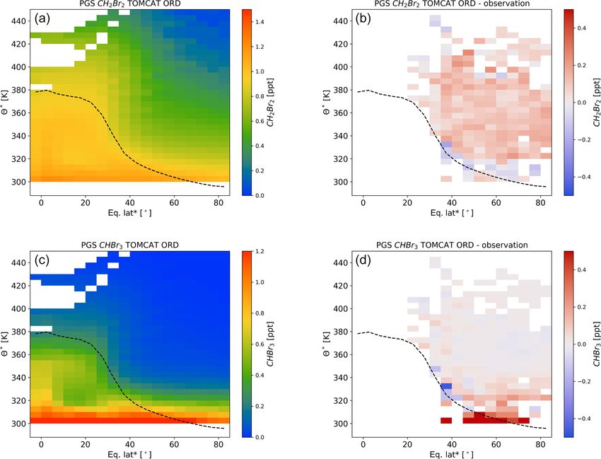
Atmos. Chem. Phys., 20, 4105–4132, 2020 www.atmos-chem-phys.net/20/4105/2020/T. Keber et al.: Bromine from short-lived source gases 4115 Figure 5. Altitude–latitude cross sections of CH2 Br2 (a, b) and CHBr3 (c, d) compiled from all flights during the PGS campaign from late December 2015 to March 2016 (a, c) and the TACTS WISE campaigns representative of conditions in late summer to early fall (b, d). The data are displayed as a function of θ ∗ (see description in Sect. 2) and equivalent latitude∗ . The dynamical tropopause (dashed line) has been derived from the ERA-Interim reanalysis, providing a climatological mean zonal mean value of the tropopause. from VSLS source gases to the stratosphere and also the fur- (see Sect. 2). The model data have been extracted for the ther chemical breakdown and the transport processes related time period and latitude ranges of the observations and have to the propagation of these gases in the stratosphere. As ex- been zonally averaged. Here we compare vertical profiles, plained in Sect. 2, we used two different models with dif- latitude–altitude cross sections and latitudinal gradients be- ferent emission scenarios for the brominated very-short-lived tween our observations and the model results in a similar way source gases. The ESCiMo simulation results from the chem- as the observations have been presented in Sect. 3. We also istry climate model EMAC (Jöckel et al., 2016) are based on compare results for total organic bromine. Only the scenar- the emission scenario by Warwick et al. (2006), while the ios of Warwick et al. (2006) and Ordóñez et al. (2012) con- TOMCAT model (Hossaini et al., 2013) was run with three tain emissions of the mixed bromochlorocarbons CH2 BrCl, different emission scenarios (Ordóñez et al., 2012; Ziska et CHBrCl2 and CHBr2 Cl. For the calculation of total VSLS or- al., 2013; Liang et al., 2010). Both models have been used in ganic bromine, based on the emission scenarios by Liang et the past to investigate the effect of brominated VSLS on the al. (2010) and Ziska et al. (2013), we have adopted the results stratosphere (e.g. Sinnhuber and Meul, 2015; Hossaini et al., from the TOMCAT model using the emissions by Ordóñez et 2012, 2015; Wales et al., 2018; Graf, 2017). For the EMAC al. (2012). The contribution from these mixed bromochloro- model, we have chosen to use results from a so-called “spec- carbons to total VSLS organic bromine is typically on the or- ified dynamics” simulation, which has been extended from der of 20 %, while about 80 % of total VSLS organic bromine the ESCiMo simulations to cover our campaign time period in the upper troposphere and lower stratosphere is due to www.atmos-chem-phys.net/20/4105/2020/ Atmos. Chem. Phys., 20, 4105–4132, 2020
4116 T. Keber et al.: Bromine from short-lived source gases
Figure 6. Latitudinal cross section of CH2 Br2 (a), CHBr3 (b) and total organic VSLS bromine (c) for all three campaigns, binned by latitude
and averaged within 10 K below the local dynamical tropopause. Also included are the reference mixing ratios for the tropical tropopause
(Engel and Rigby, 2018).
CH2 Br2 and CHBr3 . This relative contribution of 20 % from tween model potential temperature and the potential temper-
minor VSLS is found in our observations (Tables 3 and 4) ature of the climatological zonal mean tropopause, which has
as well as in the values compiled in Engel and Rigby (2018) been derived as explained in Sect. 2. As we are comparing
(see Table 5), and it is slightly larger than that derived, for our observations to the models in tropopause relative coordi-
example, in Fernandez et al. (2014). nates, we have also compared this climatological tropopause
with the tropopause derived from the EMAC model results
4.1 Mean vertical profiles for the time of our campaigns. The potential temperature of
the EMAC tropopause and the climatological tropopause dif-
fered by less than 3 K for all campaigns at mid latitudes.
Observed vertical profiles are available up to the maximum
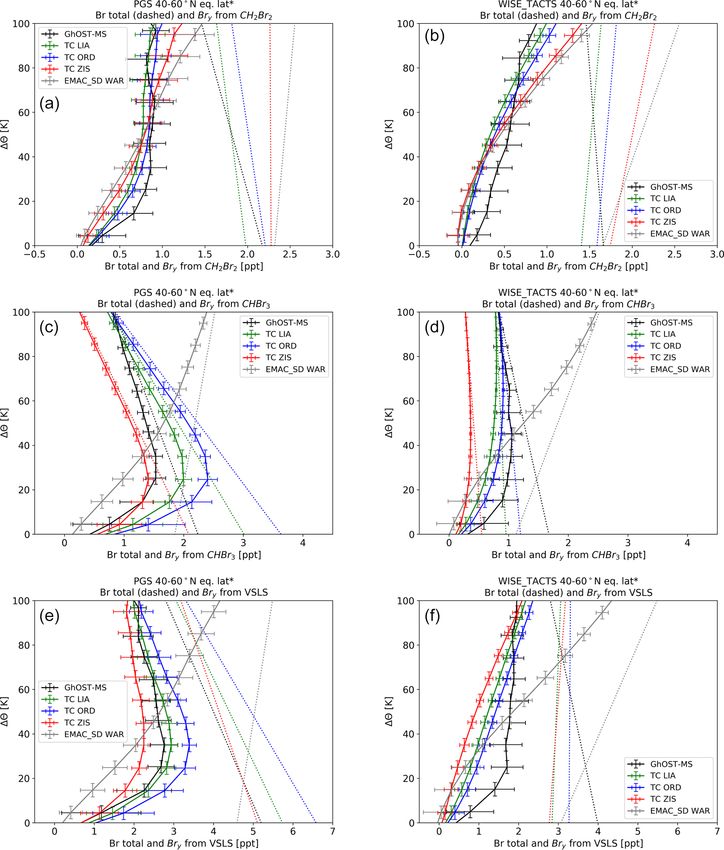
Figure 7 presents the model–measurement comparisons
flight altitude of HALO, which is about 15 km, correspond-
for the two main VSLS bromine source gases for the winter
ing to about 400 K in potential temperature. Due to the vari-
PGS campaign and for the combined dataset from WISE and
ability of the tropopause potential temperature, this translates
TACTS. A similar figure for the minor VSLS is shown in the
into a maximum of about 100 K for 1θ . The emphasis of this
Supplement (Fig. S4). Overall the Liang et al. (2010) and the
section is on the mid latitudes of the Northern Hemisphere,
Ordoñez et al. (2012) emission scenarios give the best agree-
i.e. between 40 and 60◦ equivalent latitude∗ . All comparisons
ment with our observations of CH2 Br2 . The averaged devi-
are shown as a function of 1θ . As no direct tropopause infor-
ation is 0.1 ppt or less, averaged over all campaigns and all
mation was available for the TOMCAT output, we have cho-
stratospheric measurements in the 40–60◦ N equivalent lati-
sen to derive 1θ for this comparison from the difference be-
Atmos. Chem. Phys., 20, 4105–4132, 2020 www.atmos-chem-phys.net/20/4105/2020/T. Keber et al.: Bromine from short-lived source gases 4117 Figure 7. Vertical profiles of CH2 Br2 (a, b), CHBr3 (c, d) and total organic VSLS bromine (e, f) averaged over 40–60◦ of equivalent latitude∗ and all flights during the PGS campaign from late December 2015 to March 2016 (left-hand side) and from the combined WISE_TACTS dataset, representative of conditions in late summer to fall. Also shown are model results from the TOMCAT and EMAC model using different emission scenarios (see text for details). The data are displayed as a function of potential temperature above the dynamical tropopause. In the case when no model information on the tropopause altitude was available (TOMCAT), climatological tropopause values have been used (see text for details). www.atmos-chem-phys.net/20/4105/2020/ Atmos. Chem. Phys., 20, 4105–4132, 2020
4118                                                                 T. Keber et al.: Bromine from short-lived source gases

tude band, corresponding to a mean absolute percentage dif-       4.2   Latitude–altitude cross sections
ference (MAPD) on the order of 10 %–25 %. Using the Ziska
et al. (2013) emissions, CH2 Br2 is overestimated in the mid-     As has been shown in the comparison of the vertical pro-
latitude lowest stratosphere during both campaigns by about       files, differences between model results and observations are
0.2 ppt, corresponding to about 40 %–60 % overestimation.         found, especially in the case of the Ziska et al. (2013) emis-
The overestimation is even larger with 0.25–0.3 ppt (50 %–        sions in the TOMCAT model and in the case of the War-
70 %) when using the Warwick et al. (2006) emissions in the       wick et al. (2006) emissions in the EMAC model for the
EMAC model. As CHBr3 is nearly completely depleted in             northern hemispheric mid latitudes (40–60◦ N). To visualize
the upper part of the profiles, differences will become neg-      these differences, we present latitude–altitude cross sections
ligible there. Therefore, we only compared mixing ratios in       of the model datasets and the differences to our observations
the lowest 50 K potential temperature above the tropopause.       in Figs. 9–12. While we use equivalent latitude∗ as the lat-
In this region, the best agreement is again found with the        itudinal coordinate for the observations and θ ∗ as vertical
Liang et al. (2010) and Ordoñez et al. (2012) emission sce-       coordinate, the zonal mean data are displayed as a function
narios, with mean differences always below 0.1 ppt, corre-        of latitude and potential temperature, θ , for the model re-
sponding to a MAPD of about 20 %–30 %. Using the Ziska et         sults. The comparison is shown here for the winter dataset
al. (2013) emission scenario, we find an underestimation on       from PGS, for which the observational set covers a wide
the order of 0.05–0.1 ppt (40 %–70 %), while CHBr3 is over-       range of latitudes and also reaches very low tracer mole frac-
estimated by about 0.15 ppt (120 %–180 %) in the EMAC             tions. The comparison for the campaign in late summer to
model based on the Warwick et al. (2006) emission scenario.       fall (TACTS and WISE) gives a rather similar picture (not
   Using the Ziska et al. (2013) emission scenario, the over-     shown). The overall best agreement in the vertical profiles
estimation of CH2 Br2 and the underestimation of CHBr3            has been found for the TOMCAT model using the emission
tend to cancel out. When adding the contribution from mi-         scenarios by Liang et al. (2010) and Ordóñez et al. (2012).
nor VSLS based on the scenario by Ordóñez et al. (2012),          The latitude–altitude cross section for these two datasets is
this results in a reasonable agreement in total VSLS organic      shown in Figs. 9 and 10. Using these two emission scenarios,
bromine. The EMAC model with the Warwick et al. (2006)            the TOMCAT model tends to overestimate high-latitude tro-
emissions substantially overestimates both CH2 Br2 and            pospheric mole fractions of CHBr3 during this winter cam-
CHBr3 in the lowermost stratosphere of the mid latitudes.         paign. However, the stratospheric distribution is rather well
The vertical profiles of CH2 Br2 and CHBr3 from the EMAC          reproduced with absolute deviations to the model mostly be-
model with the Warwick et al. (2006) emission scenario is         ing below 0.1 ppt. In the case of CH2 Br2 , overall strato-
therefore completely different from the observations, show-       spheric mole fractions are slightly larger in the model re-
ing a maximum around the tropopause or even above.                sults compared to the observations. The deviations between
   We additionally compare model data from EMAC simu-             the TOMCAT model using the Ziska et al. (2010) emissions
lations using all four emission scenarios (Graf, 2017) in or-     and the EMAC model using the Warwick et al. (2006) emis-
der to investigate if the large deviation of the Warwick et       sions are substantially larger. These are shown in Figs. 11
al. (2006) emission scenario is due to the EMAC model or          and 12 again for the PGS campaign. As noted above, the
due to the specific emission scenario. These simulations are      TOMCAT model with the Ziska et al. (2013) emissions over-
only available for the time period up to 2011. This com-          estimates stratospheric CH2 Br2 , while stratospheric CHBr3
parison for the January–March period (representative for the      is reasonably well captured. The largest discrepancies be-
PGS campaign) is shown in Fig. 8 for CH2 Br2 and CHBr3 .          tween model and observations are observed in the case of
Figure 8 looks qualitatively very similar to the comparisons      the EMAC model with the Warwick et al. (2006) emissions.
in Fig. 7; i.e. both CH2 Br2 and CHBr3 using the Warwick          In this case, both CH2 Br2 and CHBr3 are overestimated in
et al. (2006) emission scenario show highest mixing ratios        the lower stratosphere.
in the lower stratosphere, and CHBr3 shows the least pro-            In the case of CHBr3 , the two emission scenarios which
nounced vertical gradients. Also, the pattern for the Ziska       have a more even distribution of emissions with latitude,
et al. (2013) emission scenario is the same, with the sec-        i.e. the emission scenarios by Liang et al. (2010) and Or-
ond highest CH2 Br2 values and lowest CHBr3 values. Dif-          doñez et al. (2012), show the best agreement with the ob-
ferences between the different models are certainly a factor      servations. The emission scenario by Warwick et al. (2006)
in the explanation of model–observation differences. How-         yields much higher mole fractions in the tropics and has
ever, it is clear that the pattern when comparing all scenarios   the poorest agreement with measurement data. The emission
in the EMAC model is similar to that described above and          scenario by Ziska et al. (2013) yields overall much lower
that differences in the emission scenarios are the main driver    CHBr3 in large parts of the atmosphere and seems to be the
of model–observation differences.                                 only set-up in which mid-latitude tropopause mixing ratios
                                                                  of CHBr3 are underestimated in comparison to our observa-
                                                                  tions. For CH2 Br2 , again the Ordoñez et al. (2012) and Liang
                                                                  et al. (2010) emission scenarios in the TOMCAT model show

Atmos. Chem. Phys., 20, 4105–4132, 2020                                            www.atmos-chem-phys.net/20/4105/2020/
You can also read