Climate Data Record (CDR) Program - Climate Algorithm Theoretical Basis Document (C-ATBD) Sea Ice Concentration
←
→
Page content transcription
If your browser does not render page correctly, please read the page content below
Climate Data Record (CDR) Program

 Climate Algorithm Theoretical Basis Document (C-ATBD)
                                                Sea Ice Concentration

CDR Program Document Number: CDRP-ATBD-0107
Configuration Item Number: 01B-11 and 01B-11a
Revision 9 / June 03, 2021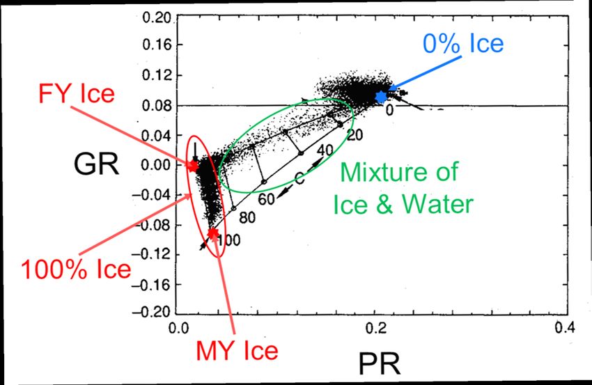
CDR Program         Sea Ice Concentration C-ATBD                          CDRP-TMP-00060107
                                                                             Rev 9 06/03/2021

                               REVISION HISTORY

Rev.   Author             DSR        Description                                  Date
                          No.
1      Walt Meier,        DSR-       Initial release.                             09/20/2011
       Research           112
       Scientist, NSIDC
2      Walt Meier,        DSR-       Added description of monthly files and       05/29/2012
       Research           204        memory allocations for processing.
       Scientist, NSIDC              Sections 3.2, 3.4.4, and 5.6.
3      Walt Meier,        DSR-       Changes made to describe Version 2           03/26/2013
       Research           411        Revision 0 of the CDR. Sections 3.2,
       Scientist, NSIDC              3.3.1, 3.4.1.4, 3.4.4.1, 3.4.4.2, and 5.6.
                                     6.1.4 (deleted)
4      Ann Windnagel,     DSR-       Changes made to describe Version 2           09/19/2015
       Professional       920        Revision 1 of the CDR. Updated Figures
       Research                      2 and 5 in Section 3.2, Sections 1.3 and
       Assistant, NSIDC              5.6, and Table 12.
5      Ann Windnagel,     DSR-       Changes made to describe Version 3           09/14/2017
       Professional       1148       and the near-real-time portion of the
       Research                      time series: Updated sections 1.1, 2.1,
       Assistant, NSIDC              2.2, 3, 4, 5.6, 6, and 8.
6      Ann Windnagel,     DSR-       Changes made to describe Version 3           12/20/2017
       Professional       1216       Revision 1. Updated sections 3.2, 3.3,
       Research                      and 3.4. Changes made to address
       Assistant, NSIDC              Version 3.1: Updated section 3.3.1.
7      Ann Windnagel,     DSR-       Changes made to tables 3, 4, and 5:          03/06/2018
       Professional       1240       instruments for the input data were
       Research                      changed from SMMIS and SMM/I to
       Assistant, NSIDC              SSMIS and SSM/I.
8      Ann Windnagel,     DSR-       Made major updates to the entire             04/19/2021
       Professional       1525       document to reflect the new Version 4
       Research                      TCDR and Version 2 ICDR release.
       Assistant, NSIDC
9      Ann Windnagel,     DSR-       Minor revision due to typographical          06/03/2021
       Professional       1527       errors
       Research
       Assistant, NSIDC

                                                                                         Page 1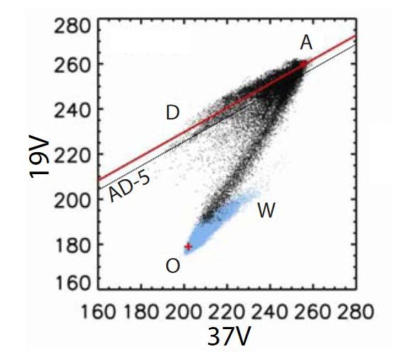
CDR Program                        Sea Ice Concentration C-ATBD                                                             CDRP-TMP-00060107
                                                                                                                               Rev 9 06/03/2021

                                                    TABLE of CONTENTS

1.    INTRODUCTION ...................................................................................................... 6
1.1     Purpose ............................................................................................................................................. 6
1.2     Definitions.......................................................................................................................................... 6
1.3     Referencing this Document ............................................................................................................... 7
1.4     Document Maintenance .................................................................................................................... 7

2.    OBSERVING SYSTEMS OVERVIEW ...................................................................... 8
2.1     Products Generated .......................................................................................................................... 8
2.2     Instrument Characteristics ................................................................................................................ 8

3.    ALGORITHM DESCRIPTION................................................................................. 11
3.1     Algorithm Overview ......................................................................................................................... 11
3.2     Processing Outline .......................................................................................................................... 11
3.2.1     Daily Processing.......................................................................................................................... 13
3.2.2     Monthly Processing ..................................................................................................................... 15
3.3     Algorithm Input ................................................................................................................................ 15
3.3.1     Primary Sensor Data ................................................................................................................... 15
3.3.2     Ancillary Data .............................................................................................................................. 18
3.3.3     Derived Data ............................................................................................................................... 19
3.3.4     Forward Models........................................................................................................................... 19
3.4     Theoretical Description ................................................................................................................... 19
3.4.1     Physical and Mathematical Description ...................................................................................... 20
3.4.2     Data Merging Strategy ................................................................................................................ 35
3.4.3     Look-Up Table Description.......................................................................................................... 36
3.4.4     Algorithm Output ......................................................................................................................... 39

4.    TEST DATASETS AND OUTPUTS ....................................................................... 53
4.1     Test Input Datasets ......................................................................................................................... 53
4.2     Test Output Analysis ....................................................................................................................... 53
4.2.1     Reproducibility ............................................................................................................................. 53
4.2.2     Precision and Accuracy............................................................................................................... 53
4.2.3     Error Budget ................................................................................................................................ 54

5.    PRACTICAL CONSIDERATIONS.......................................................................... 56
5.1     Numerical Computation Considerations ......................................................................................... 56
5.2     Programming and Procedural Considerations ................................................................................ 56
5.3     Quality Assessment and Diagnostics .............................................................................................. 56
5.4     Exception Handling ......................................................................................................................... 56
5.5     Algorithm Validation and Error Assessment ................................................................................... 56
5.5.1     Errors from sensor characteristics and gridding scheme ............................................................ 57
5.5.2     Errors due to surface variation and ambiguities.......................................................................... 59
5.5.3     Errors due to atmospheric effects ............................................................................................... 60
5.5.4     Summary of error sources and magnitudes ................................................................................ 61
5.6     Processing Environment and Resources ........................................................................................ 61

                                                                                                                                                    Page 2
CDR Program Sea Ice Concentration C-ATBD CDRP-TMP-00060107
Rev 9 06/03/2021
6. ASSUMPTIONS AND LIMITATIONS ..................................................................... 63
6.1 Algorithm Performance ................................................................................................................... 63
6.2 Sensor Performance ....................................................................................................................... 63
7. FUTURE ENHANCEMENTS .................................................................................. 64
7.1.1 Reprocessing of SSM/I using a new version of brightness temperatures .................................. 64
7.1.2 EASE-Grid 2.0 version of sea ice CDR ....................................................................................... 64
7.1.3 New algorithm coefficients for calibration ................................................................................... 64
7.1.4 Improved pole-hole filling ............................................................................................................ 65
7.1.5 Filling remaining temporal gaps using statistical modeling ......................................................... 65
8. REFERENCES ....................................................................................................... 66
APPENDIX A - ACRONYMS AND ABBREVIATIONS ................................................. 71
LIST of FIGURES
Figure 1: Flowchart showing the overview of sea ice concentration TCDR processing.
Note that the ICDR processing is identical except that the input data is NSIDC-0080
SSMIS brightness temperatures and the output is G10016. ................................................. 12
Figure 2: Overview of main python code for the daily sea ice concentration TCDR
processing. Note that the ICDR processing is identical except that the input data is
NSIDC-0080 SSMIS brightness temperatures and the output is the daily G10016. ............ 13
Figure 3: Overview of the TCDR CDRAlgos Bootstrap and NASA Team processing code.
Note that the ICDR processing is identical except that the input data is NSIDC-0080
SSMIS spatially interpolated brightness temperatures. ........................................................ 14
Figure 4: Monthly TCDR processing. Note that the ICDR processing is identical except
that the input data is the daily G10016 data and the output is G10016 monthly data. ....... 15
Figure 5: Sample plot of GR vs. PR with typical clustering of grid cell values (small dots)
around the 0% ice (open water) point (blue star) and the 100% ice line (circled in red).
First year (FY) ice clusters at the top of the 100% ice line, and multi-year (MY) ice clusters
at the bottom. Points with a mixture of ice and water (circled in green) fall between these
two extremes. Adapted from Figure 10-2 of Steffen et al. (1992). ........................................ 22
Figure 6: Example of the relationship of the 19V vs. 37V TB (in Kelvin) used in the
Bootstrap algorithm. Brightness temperatures typically cluster around the line segments
AD (representing 100% sea ice) and OW (representing 100% open water). For points that
fall below the AD-5 line (dotted line), bootstrap uses TB relationships for 37H vs. 37V.
Adapted from Comiso and Nishio (2008). ............................................................................... 25
Page 3CDR Program Sea Ice Concentration C-ATBD CDRP-TMP-00060107
Rev 9 06/03/2021
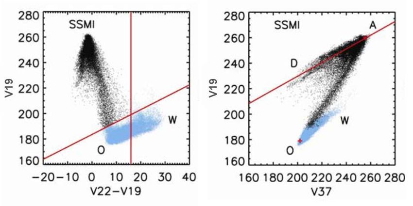
Figure 7: Sample scatter plot of 19V vs. (22V-19V) (left) and 19V vs. 37V (right) TBs.
Values shaded in blue around the OW segment are masked to 0% concentration. From
Comiso and Nishio (2008). ....................................................................................................... 30
Figure 8: Example of grid cell neighbor to define coastal proximity classification for a
grid cell, (I,J). From Cavalieri et al. (1999). ............................................................................. 31
Figure 9: Schematic of grid cell values used in calculation of the CDR standard deviation
field. All non-missing ocean/sea ice concentration values (C), from both the NASA Team
and Bootstrap algorithm, of the 3 x 3 box surrounding each (I,J) grid cell (up to 18 total
values) are used to calculate the standard deviation. A minimum of six grid cells with
valid values is used as a threshold for a valid standard deviation. ..................................... 42
LIST of TABLES
Table 1: Comparison of Nimbus and DMSP orbital parameters ............................................. 9
Table 2: IFOV of SMMR, SSM/I, and SSMIS frequencies used in the sea ice concentration
CDR algorithm (Gloersen and Barath, 1977; Hollinger et al., 1990; Kunkee et al., 2008) ... 10
Table 3: Version history and dates of the instruments used for the input brightness
temperatures for the sea ice CDR variable. ............................................................................ 17
Table 4: Brightness temperature sources and channel frequencies used for the sea ice
CDR. ........................................................................................................................................... 18
Table 5: Tie-point values (in Kelvin) for each SSM/I and SSMIS sensor along with original
SMMR values. The þ column is the additional adjustment required for open water tie-
points (no adjustment was needed for F17 or F18). .............................................................. 24
Table 6. GR3719 and Gr2219 criteria by instrument and hemisphere ................................. 29
Table 7: CDR land/coast/shore mask values. ......................................................................... 37
Table 8. Arctic Pole Hole Sizes by Instrument ....................................................................... 38
Table 9: Sea ice concentration variables flag values ............................................................ 40
Table 10: List of flag values used in the daily CDR QA field. A grid cell that satisfies more
than one criteria will contain the sum of all applicable flag values. For example, where the
Bootstrap weather filter and land spillover are applied, the flag value will be 5 (1 for BT
weather plus 4 for BT land spillover). ..................................................................................... 45
Table 11. Spatial interpolation flag values. A grid cell that satisfies more than one criteria
will contain the sum of all applicable flag values. ................................................................. 46
Page 4CDR Program Sea Ice Concentration C-ATBD CDRP-TMP-00060107
Rev 9 06/03/2021
Table 12: List of flag values used in the monthly CDR QA bit mask. A grid cell that
satisfies more than one criteria will contain the sum of all applicable flag values. For
example, if spatial interpolation was performed and melt detected then the value will be
160 (32 + 128). ........................................................................................................................... 51
Table 13: Possible error sources and magnitudes for the sea ice CDR .............................. 55
Table 14: List of error sources and typical magnitudes for the NASA Team (NT) and
Bootstrap (BT) algorithms with biases and typical regimes. ............................................... 61
Table 15: Code package and input/output memory requirements ....................................... 62
Page 5CDR Program Sea Ice Concentration C-ATBD CDRP-TMP-00060107
Rev 9 06/03/2021
1. Introduction
1.1 Purpose
The purpose of this document is to describe the sea ice climate data record (CDR)
algorithm (Meier et al. 2014; Peng et al. 2013). Beginning in 2015, updates are
submitted to the National Centers for Environmental Information (NCEI) by Florence
Fetterer at the National Snow and Ice Data Center (NSIDC).
The CDR algorithm is used to create the Sea Ice Concentration CDR from passive
microwave data from the Scanning Multichannel Microwave Radiometer (SMMR) on the
Nimbus 7 satellite and the Special Sensor Microwave/Imager (SSM/I) and the Special
Sensor Microwave Imager and Sounder (SSMIS) sensors on U.S. Department of
Defense Meteorological Satellite Program (DMSP) platforms. The goal of the Sea Ice
Concentration CDR is to provide a consistent, reliable, and well-documented product
that meets CDR guidelines as defined in Climate Data Records from Environmental
Satellites (NAS, 2004). This product is supplied in two parts. A final product that is
created from quality controlled input data available from NSIDC as the NOAA/NSIDC
Climate Data Record of Passive Microwave Sea Ice Concentration
(https://nsidc.org/data/g02202), and a near-real-time provisional product that is created
from provisional input data available from NSIDC as the Near-Real-Time NOAA/NSIDC
Climate Data Record of Passive Microwave Sea Ice Concentration
(https://nsidc.org/data/g10016). The near-real-time provisional product is provided to
users until the release of the finalized Sea Ice Concentration CDR (NOAA data set ID
01B-11, NSIDC data set ID G02202), which is available with an approximate three to six
month latency.
The algorithm is defined in the computer program (code) that accompanies this
document; and thus, the intent here is to provide a guide to understanding that
algorithm, from both a scientific perspective and a software engineering perspective in
order to assist in evaluation of the code.
1.2 Definitions
Following is a summary of the symbols used to define the algorithm.
TB = brightness temperature = ε*T (1)
ε = emissivity (2)
T = physical temperature (3)
PR = polarization ratio (4)
GR = gradient ratio (5)
Page 6CDR Program Sea Ice Concentration C-ATBD CDRP-TMP-00060107
Rev 9 06/03/2021
1.3 Referencing this Document
This document should be referenced as follows:
Sea Ice Concentration - Climate Algorithm Theoretical Basis Document, NOAA Climate
Data Record Program CDRP-ATBD-0107 Rev. 8 (2021). Available at
https://www.ncdc.noaa.gov/cdr/oceanic/sea-ice-concentration.
1.4 Document Maintenance
This is the ATBD for the Sea Ice Concentration Climate Data Record, Version 4,
Revision 0 and the Near-Real-Time Sea Ice Concentration Climate Data Record,
Version 2, Revision 0. The source code is used to create both products.
Page 7CDR Program Sea Ice Concentration C-ATBD CDRP-TMP-00060107
Rev 9 06/03/2021
2. Observing Systems Overview
2.1 Products Generated
The primary generated product is the Sea Ice Concentration climate data record based
on gridded brightness temperatures (TBs) from the Nimbsu-7 SMMR and the DMSP
series of SSM/I and SSMIS passive microwave radiometers. These data are an
estimate of sea ice concentration that are produced by combining concentration
estimates from two algorithms developed at the NASA Goddard Space Flight Center
(GSFC): the NASA Team algorithm (Cavalieri et al., 1984) and the Bootstrap algorithm
(Comiso, 1986). These algorithms are described in more detail in section 3 Algorithm
Description. For the finalized portion of this product, called the Thematic CDR (TCDR,
NSIDC data set ID G02202), NSIDC uses each individual algorithm to process and
combine gridded brightness temperatures from SMMR data acquired from NASA
Goddard Space Flight Center (GSFC) and swath brightness temperature data from
SSM/I and SSMIS acquired from Remote Sensing Systems, Inc. (RSS). For the near-
real-time provisional portion of this product, called the Interim CDR (ICDR, NSIDC data
set ID G10016), NSIDC uses each individual algorithm to process and combine swath
brightness temperature data from the NOAA Comprehensive Large Array-Data
Stewardship System (CLASS). See section 3.3 Algorithm Input for more information on
the input brightness temperatures.
Accompanying the concentration estimates are data quality information fields. One field
is a concentration standard deviation that indicates spatial variability and the variability
between the NASA Team and Bootstrap algorithm estimates. Grid cells with high
standard deviations indicate values with lower confidence levels. Another field includes
quality information such as melt state and proximity to the coast, regimes that tend to
have higher errors.
2.2 Instrument Characteristics
The SMMR passive microwave sensor was launch aboard the Nimbus-7 satellite in
October 1978. The SMMR sensor was a ten-channel sensor that measured
orthogonally polarized (horizontal and vertical) antenna temperature data in five
microwave frequencies: 6.6, 10.7, 18.0, 21.0, and 37.0 GHz (Gloersen and Hardis,
1978). NASA Nimbus-7 SMMR sensor, which predates DMSP and extends the total
time series to late 1978 with every-other-day concentration estimates.
The first SSM/I sensor was launched aboard the DMSP-F8 mission in 1987 (Hollinger et
al., 1990). A series of SSM/I conically-scanning sensors on subsequent DMSP satellites
has provided a continuous data stream since then. However, only sensors on the
DMSP-F8, -F11, -F13, -F17, and -F18 platforms are used in the generation of the CDR.
The SSM/I sensor has seven channels at four frequencies. The 19.4, 37.0, and 85.5
GHz frequencies are dual polarized, horizontal (H) and vertical (V); the 22.2 GHz
Page 8CDR Program Sea Ice Concentration C-ATBD CDRP-TMP-00060107
Rev 9 06/03/2021
frequency has only a single vertically polarized channel. The 85.5 GHz frequencies are
not used in the sea ice concentration algorithms.
Beginning with the launch of F16 in 2003, the SSM/I sensor was replaced by the SSMIS
sensor. The SSMIS sensor has the same 19.4, 22.2, and 37.0 GHz channels; however,
the 85.5 GHz channels on SSM/I are replaced with 91.0 GHz channels on SSMIS
(Kunkee et al., 2008), which is not used in the algorithms. The SSMIS sensor also
includes several higher frequency sounding channels that are not used for the sea ice
products and are not archived at NSIDC.
For simplicity, the channels are sometimes denoted as simply 18H, 18V, 19H, 19V,
22V, 37H, and 37V. Depending on the platform, the satellite altitudes are 830 to 955 km
and sensor (earth incidence) angles are 50.2 to 53.4 degrees. See Table 1 for details of
each platform.
Parameter Nimbus-7 DMSP-F8 DMSP-F11 DMSP-F13 DMSP-F17 DMSP-F18
Nominal 955 860 830 850 855 833
Altitude
(km)*
Inclination 99.1 98.8 98.8 98.8 98.8 98.6
Angle
(degrees)
Orbital 104 102 101 102 102 102
Period
(minutes)
Ascending 12:00 P.M. 6:00 A.M. 5:00 P.M. 5:43 P.M. 5:31 P.M. 8:00 P.M.
Node
Equatorial
Crossing
(approxima
te local
time)
Algorithm 18.0, 37.0 19.4, 37.0 19.4, 37.0 19.4, 37.0 19.4, 37.0 19.4, 37.0
Frequencie
s (GHz)*
Earth 50.2 53.1 52.8 53.4 53.1 53.1
Incidence
Angle
(degrees)*
Table 1: Comparison of Nimbus and DMSP orbital parameters
*Indicates sensor and spacecraft orbital characteristics of the three sensors used in generating
the sea ice concentrations.
Page 9CDR Program Sea Ice Concentration C-ATBD CDRP-TMP-00060107
Rev 9 06/03/2021
A polar orbit and wide swath provides near-complete coverage at least once per day in
the polar regions except for a small region around the North Pole called the pole hole.
The SSMIS sensor has a wider swath width (1700 km) compared to the SSM/I sensor
(1400 km), which reduces the size of the pole hole. The footprint or instantaneous field
of view (IFOV) of the sensor varies with frequency (Table 2).
Frequency (GHz) SMMR (km) SSM/I (km) SSMIS (km)
18.0/19.35 55 x 41 69 x 43 72 x 44
21.0/22.235 46 x 30 60 x 40 72 x 44
37.0 27 x 18 37 x 28 44 x 26
Table 2: IFOV of SMMR, SSM/I, and SSMIS frequencies used in the sea
ice concentration CDR algorithm (Gloersen and Barath, 1977; Hollinger
et al., 1990; Kunkee et al., 2008)
Regardless of footprint size, the low frequency channels (19.4 – 37.0 GHz) are gridded
to a 25 km polar stereographic grid.
Page 10CDR Program Sea Ice Concentration C-ATBD CDRP-TMP-00060107
Rev 9 06/03/2021
3. Algorithm Description
3.1 Algorithm Overview
The Sea Ice Concentration CDR algorithm uses concentration estimates derived at
NSIDC from the NASA Team (Cavalieri et al., 1984) and Bootstrap (Comiso, 1986)
algorithms as input data and merges them into a combined single concentration
estimate based on the known characteristics of the two algorithms. First, the Bootstrap
10% concentration threshold is used as a cutoff to define the limit of the ice edge.
Second, within the ice edge, the higher of the two concentration estimates from the
NASA Team and Bootstrap algorithms is used for the CDR input value. The reason for
these two approaches is discussed further in section Sea Ice Concentration Climate
Data Record Algorithm. Automated quality control measures are implemented
independently on the NASA Team and Bootstrap outputs. Two weather filters (one for
each algorithm), based on ratios of channels sensitive to enhanced emission over open
water, are used to filter weather effects. Separate land-spillover corrections are used for
each of the algorithms to filter out much of the error due to mixed land/ocean grid cells.
Finally, valid ice masks are applied to screen out errant retrievals of ice in regions
where sea ice never occurs.
3.2 Processing Outline
The following flow diagram (Figure 1) describe the general processing for the finalized
daily and monthly TCDR sea ice concentrations and the near-real-time provisional daily
and monthly ICDR sea ice concentrations.
Page 11CDR Program Sea Ice Concentration C-ATBD CDRP-TMP-00060107
Rev 9 06/03/2021
Figure 1: Flowchart showing the overview of sea ice concentration TCDR
processing. Note that the ICDR processing is identical except that the
input data is NSIDC-0080 SSMIS brightness temperatures and the
output is G10016.
Page 12CDR Program Sea Ice Concentration C-ATBD CDRP-TMP-00060107
Rev 9 06/03/2021
3.2.1 Daily Processing
The following flow diagrams (Figure 2 and Figure 3) describe the processing of the daily
CDR sea ice concentration in detail.
Figure 2: Overview of main python code for the daily sea ice
concentration TCDR processing. Note that the ICDR processing is
identical except that the input data is NSIDC-0080 SSMIS brightness
temperatures and the output is the daily G10016.
Page 13CDR Program Sea Ice Concentration C-ATBD CDRP-TMP-00060107
Rev 9 06/03/2021
Figure 3: Overview of the TCDR CDRAlgos Bootstrap and NASA Team
processing code. Note that the ICDR processing is identical except that
the input data is NSIDC-0080 SSMIS spatially interpolated brightness
temperatures.
Page 14CDR Program Sea Ice Concentration C-ATBD CDRP-TMP-00060107
Rev 9 06/03/2021
3.2.2 Monthly Processing
The following flow diagram (Figure 4) describes the processing of the monthly CDR sea
ice concentration for the finalized TCDR data and the near-real-time ICDR data.
Figure 4: Monthly TCDR processing. Note that the ICDR processing is
identical except that the input data is the daily G10016 data and the
output is G10016 monthly data.
3.3 Algorithm Input
3.3.1 Primary Sensor Data
Calibrated and gridded brightness temperatures from Nimbus-7 SMMR, DMSP SSM/I,
and DMSP SSMIS passive microwave sensors are used as the primary input data for
this sea ice concentration CDR. The brightness temperature data for the finalized TCDR
and near-real-time ICDR portions of the product are obtained from two different data
storage facilities: RSS and CLASS, respectively. Both the RSS and CLASS use
Page 15CDR Program Sea Ice Concentration C-ATBD CDRP-TMP-00060107
Rev 9 06/03/2021
enhanced processing methods to correct errors and improve calibration and geolocation
of the swath brightness temperatures. Specific processing information on the input
swath data is available from RSS (http://www.remss.com/missions/ssmi/) and CLASS
(https://www.avl.class.noaa.gov/saa/products/search?datatype_family=DMSP).
NSIDC obtains the input swath data from RSS and CLASS and then grids them onto a
25 km polar stereographic grid for both Arctic and Antarctic regions. These data sets
are publicly available through NSIDC’s web site. See Table 3 for a list of these data
sets, the temporal range, and the product they apply to.
For current processing of the TCDR, NSIDC is using Version 7 RSS DMSP SSMIS
brightness temperatures. Earlier periods use different versions (see Table 3). Because
the sea ice algorithms are intercalibrated at the product (concentration) level, the
brightness temperature version is less important because the intercalibration adjustment
includes any necessary changes due to differences in brightness temperature versions.
However, when Version 7 is available for the entire DMSP record and resources allow,
a full reprocessing will be considered.
For the processing of the ICDR, NSIDC uses DMSP SSMIS brightness temperatures
obtained from CLASS that do not have a version number associated with them. These
NRT data may contain errors and are not suitable for time series, anomalies, or trends
analyses. Near-real-time products do not undergo quality assessment and are therefore
not optimal for use in long-term climate studies. The near-real-time portion of this
product are available from NSIDC as the Near-Real-Time NOAA/NSIDC Climate Data
Record of Passive Microwave Sea Ice Concentration (https://nsidc.org/data/g10016).
This NRT sea ice concentration ICDR is meant as a provisional interim estimate to span
the gap before the availability of the finalized sea ice concentration TCDR, which have
an approximate three to six month latency before they are available from NSDIC as the
NOAA/NSIDC Climate Data Record of Passive Microwave Sea Ice Concentration
(https://nsidc.org/data/g02202). However, once the RSS brightness temperatures
become available, the finalized portion of the CDR is processed, which replaces the
near-real-time portion. Table 3 shows the instruments used for the input data for the
CDR.
Sensor Temporal Range Source/Data Product it NSIDC Data Product
Version Applies to
DMSP- Near-real-time CLASS (no ICDR https://nsidc.org/data/nsidc-
F18 version 0080
SSMIS given)
DMSP- 01 Jan 2008 – most RSS V7 TCDR https://nsidc.org/data/nsidc-
F17 current processing 0001
SSMIS date
DMSP- 01 Oct 1995 – 31 RSS V4 TCDR https://nsidc.org/data/nsidc-
F13 Dec 2007 0001
SSM/I
Page 16CDR Program Sea Ice Concentration C-ATBD CDRP-TMP-00060107
Rev 9 06/03/2021
DMSP- 03 Dec 1991 – 30 RSS V3 TCDR https://nsidc.org/data/nsidc-
F11 Sep 1995 0001
SMM/I
DMSP-F8 10 Jul 1987 – 02 Dec RSS V3 TCDR https://nsidc.org/data/nsidc-
SSM/I 1991 0001
Note: There are no data
from 3 December 1987
through 12 January 1988
due to satellite problems.
Nimbus-7 25 October 1978 – NSIDC V1 TCDR https://nsidc.org/data/nsidc-
SMMR 09 Jul 1987 0007
Table 3: Version history and dates of the instruments used for the input
brightness temperatures for the sea ice CDR variable.
The swath data are gridded onto a daily composite 25 km polar stereographic grid using
a drop-in-the-bucket method. For each grid cell, all footprints from all passes each day
whose centers fall within the grid cell are averaged together. Thus, some grid cells may
be an average of several (4 or 5) passes during a given day and some may be from
only one pass; some grid cells are typically not filled due to sensor characteristics, such
as the large footprint. Note that the polar stereographic grid is not equal area; the
latitude of the true scale (tangent of the planar grid) is 70 degrees. The Northern
Hemisphere grid is 304 columns by 448 rows, and the Southern Hemisphere grid is 316
columns by 332 rows. Further information on the polar stereographic grid used at
NSIDC can be found on the NSIDC web site on the Polar Stereographic Projection and
Grid web page (https://nsidc.org/data/polar-stereo/ps_grids.html).
The brightness temperatures are from the SMMR sensor on Nimbus-7, the SSM/I
sensors on the DMSP-F8, -F11, and -F13 platforms, and the SSMIS sensors from the
DMSP-F17 and -F18 platforms (Table 4). The rationale for using only these satellites
was made to keep the equatorial crossing times as consistent as possible to minimize
potential diurnal effects from data on sun-synchronous orbits of the DMSP satellites.
The passive microwave channels employed for the sea ice concentration product are
the 19.4, 22.2, and 37.0 GHz frequencies. The NASA Team algorithm uses the 19.35
GHz horizontal (H) and vertical (V) polarization channels and the 37.0 GHz vertical
channel. The 22.2 GHz V channel is used with the 19.4 GHz V for one of the weather
filters. The Bootstrap algorithm uses 37 GHz H and V channels and the 19.35 GHz V
channel; it also uses the 22.2 GHz V channel for a weather filter.
Page 17CDR Program Sea Ice Concentration C-ATBD CDRP-TMP-00060107
Rev 9 06/03/2021
Passive Microwave Sensor Sources for Sea Ice CDR
Ascending
Equatorial
Launch Date Swath Mean
Frequencies Crossing Time
Satellite Sensor (Data Available) Width Altitude
(GHz) At Launch
[Data at NSIDC] (km) (km)
(Most Recent,
Date)
10/24/78
NIMBUS-7 SMMR 18, 37 12:00 783 955
[10/25/78-8/20/87]
6/18/87 06:15
DMSP-F8 SSM/I 19, 22, 37 1400 840
[7/9/87-12/30/91] (06:17, 9/2/95)
11/28/91
18:11
DMSP-F11 SSM/I 19, 22, 37 (12/6/91-5/16/00) 1400 859
(18:25, 9/2/95)
[12/3/91-9/30/95]
3/24/95
17:42
DMSP-F13 SSM/I 19, 22, 37 (3/25/95-11/19/09) 1400 850
(18:33, 11/28/07)
[5/3/95-12/31/08]
11/4/06
DMSP-F17 SSMIS 19, 22, 37 (12/14/06-present) (17:31, 11/28/07) 1700 850
[1/1/07-3/31/16]]
10/18/09
DMSP-F18 SSMIS 19, 22, 37 (3/8/10-present) 20:00 1700 833
[4/1/16-present)
Table 4: Brightness temperature sources and
channel frequencies used for the sea ice CDR.
3.3.2 Ancillary Data
Ancillary data required to run the NASA team and Bootstrap algorithms: (A) land masks
imbedded within each field, based on masks developed by GSFC, (B) valid sea ice
masks to define the limits of possible sea ice, (C) a climatological minimum sea ice
mask (CMIN) (for the NASA Team only used in the land-spillover correction), and (D) a
melt onset estimate for the Northern Hemisphere to be used in the quality field. Each of
these is discussed further below.
A. Each sea ice concentration and associated fields include an embedded land
mask. See Table 7 for a description of the mask fields. Both the NASA Team and
Bootstrap algorithms use the same mask.
B. Ocean climatology masks are used to remove any remaining spurious ice not
filtered by automated corrections in regions where sea ice is not possible. There
are monthly masks for each hemisphere. For the Northern Hemisphere,
remaining spurious ice is removed using the Polar Stereographic Valid Ice Masks
Derived from National Ice Center Monthly Sea Ice Climatologies. There are 12
Page 18CDR Program Sea Ice Concentration C-ATBD CDRP-TMP-00060107
Rev 9 06/03/2021
masks, one for each month. They are available from NSIDC
(https://nsidc.org/data/nsidc-0622). The Southern Hemisphere masks, produced
from information from Goddard, are found in the ancillary directory in the code
base that is available for download from the NOAA NCEI CDR program. In
addition, there are also daily climatology ice masks derived from Bootstrap Sea
Ice Concentrations for both the Northern and Southern hemispheres. The masks
are discussed further in section 3.4.1.3 Quality Control Procedures.
C. Because of the large instantaneous field of view of the SMMR, SSM/I, and
SSMIS sensors, mixed land-ocean grid cells occur. These present a problem for
the automated concentration algorithm because the emission from the combined
land-ocean region has a signature similar to sea ice and is interpreted as such by
the algorithms. For the NASA Team algorithm, a filtering mechanism has been
implemented to automatically remove much of these false coastal ice grid cells
by using a weighting based on the proximity of the grid cell to the coast and a
minimum concentration matrix, CMIN. There is one CMIN field for each
hemisphere. The CMIN matrix is described below in Section Quality Control
Procedures.
D. A near-real-time version of a snow melt onset over sea ice field algorithm by
Drobot and Anderson (2001) is used as an input for the Northern Hemisphere
quality indicator. Liquid water over the ice changes the surface emission resulting
in errors in the algorithms, typically an underestimation of concentration. Thus,
occurrence of melt in a grid cell is an indication of lower quality.
3.3.3 Derived Data
Not applicable.
3.3.4 Forward Models
Not applicable.
3.4 Theoretical Description
Passive microwave radiation is naturally emitted by the Earth’s surface and overlying
atmosphere. This emission is a complex function of the microwave radiative properties
of the emitting body (Hallikainen and Winebrenner, 1992). However, for the purposes of
microwave remote sensing, the relationship can be described as a simple function of
the physical temperature (T) of the emitting body and the emissivity (ε) of the body.
TB = ε*T (6)
Page 19CDR Program Sea Ice Concentration C-ATBD CDRP-TMP-00060107
Rev 9 06/03/2021
TB is the brightness temperature and is the parameter (after calibrations) retrieved by
satellite sensors and is the input parameter to passive microwave sea ice concentration
algorithms.
3.4.1 Physical and Mathematical Description
The microwave electromagnetic properties of sea ice are a function of the physical
properties of the ice, such as crystal structure, salinity, temperature, or snow cover. In
addition, open water typically has an electromagnetic emission signature that is distinct
from sea ice emission (Eppler et al., 1992). These properties form the basis for passive
microwave retrieval of sea ice concentrations.
Specifically, the unfrozen water surface is highly reflective in much of the microwave
regime, resulting in low emission. In addition, emission from liquid water is highly
polarized. When salt water initially freezes into first-year (FY) ice (ice that has formed
since the end of the previous melt season), the microwave emission changes
substantially; the surface emission increases and is only weakly polarized. Over time as
freezing continues, brine pockets within the sea ice drain, particularly if the sea ice
survives a summer melt season when much of the brine is flushed by melt water. This
multi-year (MY) ice has a more complex signature with characteristics generally
between water and FY ice. Other surface features can modify the microwave emission,
particularly snow cover, which can scatter the ice surface emission and/or emit radiation
from within the snow pack. Atmospheric emission also contributes to any signal
received by a satellite sensor. These issues result in uncertainties in the retrieved
concentrations, which are discussed further below.
Because of the complexities of the sea ice surface as well as surface and atmospheric
emission and scattering, direct physical relationships between the microwave emission
and the physical sea ice concentration are not feasible. Thus, the standard approach is
to derive concentration through empirical relationships. These empirically-derived
algorithms take advantage of the fact that brightness temperature in microwave
frequencies tend to cluster around consistent values for pure surface types (100% water
or 100% sea ice). Concentration can then be derived using a simple linear mixing
equation (Zwally et al., 1983) for any brightness temperature that falls between the two
pure surface values:
TB = TICI + TO(1-CI) (7)
Where TB is the observed brightness temperature, TI is the brightness temperature for
100% sea ice, TO is the brightness temperature for open water, and CI is the sea ice
concentration.
In reality, such an approach is limited by the surface ambiguities and atmospheric
emission. Using combinations of more than one frequency and polarization limits these
effects, resulting in better discrimination between water and different ice types and a
more accurate concentration estimate.
Page 20CDR Program Sea Ice Concentration C-ATBD CDRP-TMP-00060107
Rev 9 06/03/2021
There have been numerous algorithms derived using various combinations of the
frequencies and polarizations on the SMMR and SSM/I sensors. Two commonly used
algorithms are the NASA Team (Cavalieri et al., 1984) and Bootstrap (Comiso, 1986),
both developed at NASA GSFC. The sea ice concentration CDR described here is
produced via a combination of estimates from the NASA Team algorithm and the
Bootstrap algorithm. Below, each algorithm is described in more detail followed by a
description of quality control (QC) procedures and the procedure to merge the two
algorithm estimates into the final CDR product with the sea ice concentration CDR
algorithm.
3.4.1.1 NASA Team Algorithm
The NASA Team algorithm uses brightness temperatures from the 19V, 19H, and 37V
channels (Cavalieri et al., 1984). The methodology is based on two brightness
temperature ratios, the polarization ratio (PR) and spectral gradient ratio (GR), as
defined below:
PR(19) = [TB(19V) – TB(19H))]/[TB(19V) + TB(19H)] (8)
GR(37V/19V) = [TB(37V) – TB(19V)]/[TB(37V) + TB(19V)] (9)
When PR and GR are plotted against each other, brightness temperature values tend to
cluster in two locations, an open water (0% ice) point and a line representing 100% ice
concentration, roughly forming a triangle. The concentration of a grid cell with a given
GR and PR value is calculated by a linear interpolation between the open water point
and the 100% line segment (Figure 5).
Page 21CDR Program Sea Ice Concentration C-ATBD CDRP-TMP-00060107
Rev 9 06/03/2021
Figure 5: Sample plot of GR vs. PR with typical clustering of grid cell
values (small dots) around the 0% ice (open water) point (blue star) and
the 100% ice line (circled in red). First year (FY) ice clusters at the top of
the 100% ice line, and multi-year (MY) ice clusters at the bottom. Points
with a mixture of ice and water (circled in green) fall between these two
extremes. Adapted from Figure 10-2 of Steffen et al. (1992).
Mathematically, these two ratios are combined in the following two equations:
CF = (a0 + a1PR + a2GR + a3PR * GR)/D (10)
CM = (b0 + b1PR + b2GR + b3PR * GR)/D (11)
where D = c0 + c1PR + c2GR + c3PR * GR (12)
The CF and CM parameters represent ice concentration for two different sea ice types. In
the Arctic, these generally correspond to FY ice (CF: ice that has grown since the
previous summer) and MY ice (CM: ice that has survived at least one melt season). In
the Antarctic, due to its small amount of MY ice and different ice characteristics, CM and
CF do not necessarily correspond to the age types and are simply denoted as Type A
and Type B. Total ice concentration (CT) is the sum of the two partial concentrations.
CT = CF + CM (13)
Page 22CDR Program Sea Ice Concentration C-ATBD CDRP-TMP-00060107
Rev 9 06/03/2021
The ai, bi, ci (i=0, 3) coefficients are empirically derived from nine observed TBs at each
of the 3 channels for 3 pure surface types (two sea ice and one open water). These TBs,
called tie-points, were originally derived for the SMMR sensor (Cavalieri et al., 1984).
The tie-points were adjusted for subsequent sensors via intercalibration of the
concentration/extent fields during sensor overlap periods to ensure consistency through
the time series (Cavalieri et al., 1999). Tie-point adjustments are made via a linear
regression analysis along with additional adjustments for open water tie-points. The tie-
point adjustment procedure and tie-point values for all sensors through F13 SSM/I are
provided in Cavalieri et al. (1999). Tie-points for F17 are described in Cavalieri et al.
(2011). See Table 5.
NIMBUS 7 SMMR
Arctic 18H 18V 37V
OW 98.5 168.7 199.4
FY 225.2 242.2 239.8
MY 186.8 210.2 180.8
Antarctic
OW 98.5 168.7 199.4
A 232.2 247.1 245.5
B 205.2 237.0 210.0
DMSP-F8 SSMI
Arctic 19H þ 19V þ 37V þ
OW 113.2 +0.2 183.4 +0.5 204.0 -1.6
FY 235.5 251.5 242.0
MY 198.5 222.1 184.2
Antarctic
OW 117.0 +7.7 185.3 +3.8 207.1 +5.3
A 242.6 256.6 248.1
B 215.7 246.9 212.4
DMSP-F11 SSMI
Arctic 19H þ 19V þ 37V þ
OW 113.6 +0.5 185.1 +0.5 204.8 +0.2
FY 235.3 251.4 242.0
MY 198.3 222.5 185.1
Antarctic
OW 115.7 +0.1 186.2 -0.4 207.1 -1.4
A 241.2 255.5 245.6
B 214.6 246.2 211.3 -2.0
DMSP-F13 SSMI
Page 23CDR Program Sea Ice Concentration C-ATBD CDRP-TMP-00060107
Rev 9 06/03/2021
Arctic 19H 19V 37V
OW 114.4 185.2 205.2
FY 235.4 251.2 241.1
MY 198.6 222.4 186.2
Antarctic
OW 117.0 +0.3 186.0 206.9
A 241.4 256.0 245.6
B 214.9 246.6 211.1
DMSP-F17 SSMIS
Arctic 19H 19V 37V
OW 113.4 184.9 207.1
FY 232.0 248.4 242.3
MY 196.0 220.7 188.5
Antarctic
OW 113.4 184.9 207.1
A 237.8 253.1 246.6
B 211.9 244.4 212.6
DMSP-F18 SSMIS
Arctic 19H 19V 37V
OW 113.4 184.9 207.1
FY 232.0 248.4 242.3
MY 196.0 220.7 188.5
Antarctic
OW 113.4 184.9 207.1
A 237.8 253.1 246.6
B 211.9 244.4 212.6
Table 5: Tie-point values (in Kelvin) for each SSM/I and SSMIS sensor
along with original SMMR values. The þ column is the additional
adjustment required for open water tie-points (no adjustment was
needed for F17 or F18).
The algorithm can sometimes obtain concentration values that are less than 0% or are
greater 100%, both of which are clearly unphysical. Such values are set to 0% and
100%, respectively.
3.4.1.2 Bootstrap Algorithm
Like the NASA Team algorithm, the Bootstrap algorithm is empirically derived based on
relationships of brightness temperatures at different channels. The current version of
Page 24CDR Program Sea Ice Concentration C-ATBD CDRP-TMP-00060107
Rev 9 06/03/2021
the Bootstrap algorithm is 3.1 (Comiso et al., 2017), which is used in the CDR
processing. The Bootstrap method uses the fact that scatter plots of different sets of
channels show distinct clusters that correspond to pure surface types (100% sea ice or
open water) (Comiso, 1986).
Figure 6 shows a schematic of the general relationship between two channels. Points
that fall along line segment AD represent 100% ice cover. Points that cluster around
point O represent open water (0% ice). Concentration for a point B is determined by a
linear interpolation along the distance from O to I where I is the intersection of segment
OB and segment AD. This is described by the following equation:
C = (TB-TO)/(TI-TO) (14)
Figure 6: Example of the relationship of the 19V vs. 37V TB (in Kelvin)
used in the Bootstrap algorithm. Brightness temperatures typically cluster
around the line segments AD (representing 100% sea ice) and OW
(representing 100% open water). For points that fall below the AD-5 line
(dotted line), bootstrap uses TB relationships for 37H vs. 37V. Adapted
from Comiso and Nishio (2008).
The Bootstrap algorithm uses two such combinations, 37H versus 37V and 19V versus
37V, denoted as HV37 and V1937, respectively. Points that fall within 5 K of the AD
Page 25CDR Program Sea Ice Concentration C-ATBD CDRP-TMP-00060107
Rev 9 06/03/2021
segment in a HV37 plot, corresponding roughly to concentrations > 90%, use this
approach. Points that fall below the AD-5 line, use the V1937 relationship to derive the
concentration. Slope and offset values for line segment AD were originally derived for
each hemisphere for different seasonal conditions (Table 2 in Comiso et al, 1997).
However, a newer formulation was developed where slope and offsets are derived for
each daily field based on the clustering of sea ice signatures within the daily brightness
temperatures (Comiso and Nishio, 2008). This dynamic tie point adjustment allows for
day-to-day changes in sea ice microwave characteristics. Further refinements were later
done, including adjusting open water tie points (Comiso et al., 2017). It is this latest
version of the Bootstrap algorithm (Version 3), with dynamic sea ice and open water tie
points, that is used in Version 4 of the CDR.
Intersensor calibration is done similar to the way it is done for the NASA Team algorithm
where brightness temperatures from the sensors are regressed against each other. One
sensor’s brightness temperatures are adjusted based on the regression with the other
sensor. However, because the slope and offset values are derived each day based on
the brightness temperatures, there are not specific slope/offset (tie-point) adjustments
between sensors. Also, while the NASA Team originally derived the tie-points for SMMR
and then adjusted future sensors to maintain consistency with SMMR, the newest
version of the Bootstrap algorithm used AMSR-E as a baseline and adjusted SSM/I and
SMMR brightness temperatures to be consistent with AMSR-E. Because AMSR-E is a
newer and more advanced sensor, the intersensor calibration should be more accurate
and more consistent overall. This is discussed further in Comiso and Nishio (2008) as
well as further minor improvements for the latest version in Comiso et al. (2017).
The algorithm can sometimes obtain concentration values that are less than 0% or are
greater 100%, both of which are clearly unphysical. Such values are set to 0% and
100% respectively.
3.4.1.3 Quality Control Procedures
Several automated quality control procedures have been implemented to spatially and
temporally fill in missing data and to filter out spurious concentration values.
Small amounts of missing data are common in satellite data, especially over a satellite
record spanning more than 40 years. Reasons for missing data are numerous and
range from issues with the instrument onboard the satellite, satellite viewing angles, and
problems arising at the ground stations when data are downloaded from the satellite.
These missing data are handled in two ways in the CDR processing code. First, a
spatial interpolation is performed on the input brightness temperature data to fill small
gaps (a few pixels). Then, temporal interpolation is performed on the sea ice
concentration data to fill larger gaps (full swaths or entire days). These are described
further in detail in sections below.
The main sources of the spurious ice grid cells are: ocean surface brightness
temperature variation, atmospheric emission, and mixed land-ocean IFOV in a grid cell.
Page 26CDR Program Sea Ice Concentration C-ATBD CDRP-TMP-00060107
Rev 9 06/03/2021
These are first discussed in general and then the specific filters used to remove much of
these effects are described for each of the NASA Team and Bootstrap products.
Both algorithms assume that open water can be represented as a single point in the
clustering of different channel combinations. However, it is evident in Figure 5 and
Figure 6 that there is considerable spread around the open water point. This is primarily
due to weather effects, namely: roughening of the ocean surface by winds, which
increases the microwave emission of the water; and atmospheric emission, primarily
due to water vapor and liquid water (clouds), which will also increase the emission
retrieved by the sensor. Atmospheric emission is most pronounced during rain fall over
the open ocean. Emission from the atmosphere has the largest effect on the 19.35 GHz
channels because they are near to frequencies (22.235 GHz) in which there is strong
water vapor emission.
Spurious ice is also common along ice-free coasts. Because of the large IFOV (up to 72
km x 44 km for 19.35 GHz), brightness temperature values from ocean grid cells near
the coast often contain microwave emission from both land and ocean. These mixed
grid cells of ocean/land have a brightness temperature signature that is often interpreted
by the algorithms as sea ice. When sea ice is actually present along the coast, the
effect is small, but when there is no ice present, artifacts of false ice appear. This is
commonly called the land-spillover effect because emission from the land surface “spills
over” into ocean grid cells.
Automated filters used to correct these spurious concentrations are discussed further in
sections below. It is possible, however, that the automated filters may also remove real
ice in some conditions.
Brightness Temperature Spatial Interpolation
The input brightness temperatures that are used to produce the sea ice CDR
sometimes contain small gaps in the data fields. These occur commonly in the fields,
especially in the more equator-ward parts of the grids. This is because of the drop-in-
the-bucket (DITB) method used for gridding the brightness temperature swath data. The
DITB method simply averages all footprints (swaths) into a grid in a given day based on
the center location of the footprint. For example, at each grid cell, all footprints whose
centers are within that grid cell’s boundaries are found. However, because the footprints
are larger than grid cell size, some grid cells have no footprint centers. So these are
empty grid cells (i.e., have a missing or zero value). These happen more equator-ward
because there are fewer overlapping swaths and thus more chance of empty grid cells.
These empty grid cells are generally isolated, that is, 1 or 2 missing grid cells
surrounded by cells with valid TB values. To correct for these missing grid cells, they are
filled by bilinear interpolation where by the grid cell is filled with the average of the four
grid cells that surround it: one above, one below, one to the left, and one to the right.
However, to make the spatial filling algorithm more robust and allow for filling of
neighboring missing grid cells, a threshold of at least three out of the four surrounding
Page 27CDR Program Sea Ice Concentration C-ATBD CDRP-TMP-00060107
Rev 9 06/03/2021
cells with valid values was set. A flag called spatial_interpolation_flag marks the
channels that were interpolated. See section 3.4.4.1 for more information on this flag.
This spatial interpolation is performed on all TB channels prior to the input data being
passed into the sea ice concentration algorithms. Larger gaps in the data are filled by
temporal interpolation (see the section below).
Sea Ice Concentration Temporal Interpolation
To fill larger gaps in the data such as missing swaths or missing days of data, a
temporal interpolation is performed on the sea ice concentration data. Once the TBs are
processed through the NASA Team and Bootstrap sea ice algorithms, the temporal
interpolation is applied. The method of interpolation is performed by locating a missing
sea ice concentration grid cell on a particular date and then using linear interpolation to
fill that value from data on either side of that date. Data can be interpolated with values
of up to five days on either side of the missing date and those days do not have to be
evenly spaced on either side. For example, a missing grid cell can be interpolated from
a data point one day in the past and one day in the future or a data point two days in the
past and four days in the future up to a data point five days in the past and five days in
the future. This linear interpolation method is the preferred technique of temporal
interpolation. However, in some cases, gaps still exist after this interpolation scheme is
performed because two data points on either side of the missing value are not found
with which to linear interpolate. To attempt to further fill these gaps, a single-sided gap
filling is performed whereby we check if there is at least one data value up to three days
on either side of the date and then simply copy that value into the missing grid cell. A
flag called temporal_interpolation_flag marks the data that were interpolated. See
section 3.4.4.1 for more information on this flag.
Pole Hole Spatial Interpolation
A polar orbit and wide swath provides near-complete coverage at least once per day in
the polar regions except for a small region around the North Pole called the pole hole.
The size of this hole has changed through time as the instruments have advanced. See
Table 8 for a list of the sizes of the holes by instrument. A spatial interpolation has been
applied to the pole hole to fill this area. The method involves averaging all sea ice
concentration grid cell values that surround the hole and then filling the missing grid
cells within the hole with that average. Thus, all grid cells within the pole hole have the
same concentration value. This interpolation is done on the NASA Team and Bootstrap
sea ice concentrations after they have been temporally interpolated. A value of 32 is set
in the spatial_interpolation_flag variable identifying this region as being interpolated.
See section 3.4.4.1 for more information on this flag.
Note: The current pole hole is quite small (Table 8); and even though the ice edge has
retreated a lot in recent years, the hole is still well within the boundary of where we are
confident that ice exists. However, it is important to note that one cannot assume what
the concentration is, especially in late Arctic summer and early autumn. Thus, we would
Page 28CDR Program Sea Ice Concentration C-ATBD CDRP-TMP-00060107
Rev 9 06/03/2021
advise caution in using the interpolated data in long-term trends or climatology analyses
and would generally recommend against it. For time series analysis (trends), users
should still apply the pole hole mask (see section 3.4.3.3). We are filling the hole to
provide a complete field for users that want/need complete fields without gaps (e.g.,
modelers).
NASA Team Weather Filters
Spurious ice over open water is removed by a threshold of the GR3719 ratio (Equation
9) and an additional GR2219 ratio:
GR(22V/19V) = [TB(22V) – TB(19V)]/[TB(22V) + TB(19V)] (15)
Using the following criteria listed in Table 6:
Instrument Hemisphere Criteria
SMMR Northern GR3719 > 0.070 concentration = 0
GR2219 N/A
SMMR Southern GR3719 > 0.076 concentration = 0
GR2219 N/A
SSM/I Northern GR3719 > 0.050 concentration = 0
GR2219 > 0.045 concentration = 0
SSM/I Southern GR3719 > 0.050 concentration = 0
GR2219 > 0.045 concentration = 0
SSMIS Northern GR3719 > 0.050 concentration = 0
GR2219 > 0.045 concentration = 0
SSMIS Southern GR3719 > 0.057 concentration = 0
GR2219 > 0.045 concentration = 0
Table 6. GR3719 and Gr2219 criteria by instrument and hemisphere
Note that NASA Goddard uses a GR3719 threshold of 0.053 for SSMIS in the Southern
Hemisphere, and a GR3719 threshold of 0.076 for SMMR in the Southern Hemisphere.
While creating the Version 4 sea ice CDR, it was found that slightly adjusting those
thresholds led to better agreement in the satellite transitions for the CDR product.
Bootstrap Weather Filters
The Bootstrap algorithm also uses combinations of 19V, 22V, and 37V as a weather
filter, but the methodology follows the overall Bootstrap by thresholding above a cluster
of points in (1) 19V vs. 37V, and (2) 19V vs. (22V-19V) TB scatter plots (Figure 7).
Page 29You can also read