Depth Estimation from Light Field Geometry Using Convolutional Neural Networks
←
→
Page content transcription
If your browser does not render page correctly, please read the page content below
sensors
Article
Depth Estimation from Light Field Geometry Using
Convolutional Neural Networks †
Lei Han * , Xiaohua Huang, Zhan Shi and Shengnan Zheng

                                          School of Computer Engineering, Nanjing Institute of Technology, Nanjing 211167, China;
                                          xiaohuahwang@gmail.com (X.H.); shiz@njit.edu.cn (Z.S.); zhengsn@njit.edu.cn (S.Z.)
                                          * Correspondence: hanl@njit.edu.cn
                                          † This paper is an extended version of Han, L.; Huang, X.; Shi, Z.; Zheng, S. Learning Depth from Light Field via
                                            Deep Convolutional Neural Network. In Proceedings of the 2nd International Conference on Big Data and
                                            Security (ICBDS), Singapore, 20–22 December 2020.

                                          Abstract: Depth estimation based on light field imaging is a new methodology that has succeeded
                                          the traditional binocular stereo matching and depth from monocular images. Significant progress has
                                          been made in light-field depth estimation. Nevertheless, the balance between computational time
                                          and the accuracy of depth estimation is still worth exploring. The geometry in light field imaging is
                                          the basis of depth estimation, and the abundant light-field data provides convenience for applying
                                          deep learning algorithms. The Epipolar Plane Image (EPI) generated from the light-field data has a
                                          line texture containing geometric information. The slope of the line is proportional to the depth of
                                          the corresponding object. Considering the light field depth estimation as a spatial density prediction
                                          task, we design a convolutional neural network (ESTNet) to estimate the accurate depth quickly.
                                          Inspired by the strong image feature extraction ability of convolutional neural networks, especially
                                for texture images, we propose to generate EPI synthetic images from light field data as the input
                                   of ESTNet to improve the effect of feature extraction and depth estimation. The architecture of
Citation: Han, L.; Huang, X.; Shi, Z.;    ESTNet is characterized by three input streams, encoding-decoding structure, and skipconnections.
Zheng, S. Depth Estimation from           The three input streams receive horizontal EPI synthetic image (EPIh), vertical EPI synthetic image
Light Field Geometry Using                (EPIv), and central view image (CV), respectively. EPIh and EPIv contain rich texture and depth cues,
Convolutional Neural Networks.            while CV provides pixel position association information. ESTNet consists of two stages: encoding
Sensors 2021, 21, 6061. https://          and decoding. The encoding stage includes several convolution modules, and correspondingly,
doi.org/10.3390/s21186061
                                          the decoding stage embodies some transposed convolution modules. In addition to the forward
                                          propagation of the network ESTNet, some skip-connections are added between the convolution
Academic Editor: Paweł Pławiak
                                          module and the corresponding transposed convolution module to fuse the shallow local and deep
                                          semantic features. ESTNet is trained on one part of a synthetic light-field dataset and then tested
Received: 15 July 2021
Accepted: 7 September 2021
                                          on another part of the synthetic light-field dataset and real light-field dataset. Ablation experiments
Published: 10 September 2021              show that our ESTNet structure is reasonable. Experiments on the synthetic light-field dataset and
                                          real light-field dataset show that our ESTNet can balance the accuracy of depth estimation and
Publisher’s Note: MDPI stays neutral      computational time.
with regard to jurisdictional claims in
published maps and institutional affil-   Keywords: depth estimation; deep learning; light field; EPI; convolutional neural network; textu-
iations.                                  ral image

Copyright: © 2021 by the authors.         1. Introduction
Licensee MDPI, Basel, Switzerland.             Estimating depth information is a crucial task in computer vision [1]. Many challeng-
This article is an open access article    ing computer vision problems have proven to benefit from incorporating depth information,
distributed under the terms and           including 3D reconstruction, semantic segmentation, scene understanding, and object de-
conditions of the Creative Commons        tection [2]. Recently, depth from the light field has become one of the new hotspots, as
Attribution (CC BY) license (https://
                                          light-field imaging captures much more information on the angular direction of light rays
creativecommons.org/licenses/by/
                                          compared to monocular or binocular imaging [1]. The plenoptic cameras such as Lytro and
4.0/).

Sensors 2021, 21, 6061. https://doi.org/10.3390/s21186061                                                      https://www.mdpi.com/journal/sensors
Sensors 2021, 21, 6061                                                                                          2 of 17

                         Raytrix facilitate the data acquirement of a light field. Refocusing images, sub–aperture
                         images, and epipolar plane images (EPIs) can be generated from the light field data. Many
                         new methods of depth estimation have emerged based on these derived images. Especially,
                         EPI-based depth estimation is more popular.
                               EPIs exhibit a particular internal structure: every captured scene point corresponds to
                         a linear trace in an EPI, where the slope of the trace reflects the scene point’s distance to
                         the camera [3]. Some methods have obtained depth maps by optimizing the slope metric
                         of straight lines in EPIs, and standard feature metrics include color variance, 4D gradient,
                         structure tensor, etc. It is challenging to model the occlusion, noise, and homogeneous
                         region using feature metrics, so the accuracy of these methods is limited. Furthermore,
                         the global optimization process is always computationally expensive, which hampers its
                         practical usage.
                               With the rise of deep learning, some efforts have integrated feature extraction and
                         optimization into a unified framework of convolutional neural networks, achieving good
                         results. These advances are due to the feature extraction capability of deep neural networks.
                         The research shows that convolutional neural networks are very good at feature extraction
                         of texture images [4]. However, the current depth estimation methods based on deep
                         learning seldom directly use rich texture features in EPIs. Moreover, some methods
                         use complex network structures with many parameters and less consideration of the
                         computational cost. Taking EPINet [5] as an example, it shows good performance against
                         the HCI (Heidelberg Collaboratory for Image Processing) benchmark. However, the depth
                         map resolution obtained by EPINet is lower than that of the central view image. It is not
                         wholly pixel-wise prediction or lightweight.
                               In this paper, we focus on designing a novel neural network that directly utilizes tex-
                         tural features of EPIs based on epipolar geometry and balances depth estimation accuracy
                         and computational time. Our main contribution is twofold:
                         •    EPI synthetic images: We stitch EPIs row by row or column by column to generate
                              horizontal or vertical EPI synthetic images with more obvious texture. The two EPI
                              synthetic images, as well as the central view image, are used as the multi-stream
                              inputs of our network. In this way, a convolutional neural network (CNN) can play
                              an essential role in texture feature extraction and depth-estimation accuracy. As far
                              as we know, our work is the first to use EPI synthetic image as the input of a depth
                              estimation network. In terms of multi-stream inputs, our network is significantly
                              different from EPINet [5], which takes the sub-aperture image stack as the input of
                              each stream, whereas we use EPI synthetic images.
                         •    New CNN architecture for end-to-end lightweight computing: We employ skip-
                              connections to fuse structural information in shallow layers and semantic information
                              in deep layers to reduce our network parameters and computational time. Further-
                              more, transposed convolution modules are used to improve the resolution of the
                              output disparity map in order to be consistent with the central view image, thus
                              forming an end-to-end training model and cutting down training complexity.
                               As an extended version of our conference paper [6], this paper enriches the principle
                         description and experimental verification. The remainder of the paper is organized as
                         follows. Section 2 reports related studies on depth estimation using EPIs from the light
                         field. Section 3 describes the geometric principle and synthetic texture used in our method.
                         Section 4 details our network architecture, including the general framework, multi-stream
                         inputs, skip-connections, and the loss function used in training. Section 5 presents the
                         experiments performed and discusses the results. Finally, Section 6 concludes this paper.

                         2. Related Work
                              In the following, we briefly introduce existing approaches, focusing our description
                         on the light-field depth estimation methods using EPIs. According to different technical
                         principles, EPI-based depth estimation methods can be divided into two types: EPI analysis
                         and deep learning.
Sensors 2021, 21, 6061                                                                                             3 of 17

                               EPI analysis-based methods extract depth information from the light field by evaluat-
                         ing the directions of the lines in EPIs. The idea is to try out all the different directions: the
                         one with the least color variance along the line is most likely to give the correct depth value.
                         Based on this point, several methods use different ways to measure color variance. Kim
                         et al. employed a modified Parzen window estimation with an Epanechenikov kernel [3].
                         Tao et al. [7] used the standard deviation to measure correspondence cues, then combined
                         this with the defocus cue to calculate depth. Since all EPI data has a similar gradient pattern,
                         it is unnecessary to try out all hypothetical depth values to find the optimal. Accordingly,
                         Mun et al. [8] efficiently reduced the number of angular candidates for cost computation.
                               Similarly, Han et al. [9] select only eight sub-aperture images with different directions
                         to compute stereo disparity and fuse stereo disparity and defocus response, based on
                         guided filtering, to produce high-quality depth maps. Other EPI-analysis-based methods
                         employ gradient or a structural tensor. For example, Wanner and Goldluecke [10] applied
                         the 2D structure tensor to measure the direction of each position in the EPIs. Li et al. [11]
                         used the depth estimation from the structure tensor as a starting point, followed by a
                         refinement step based on examining the color correspondence along the detected line
                         from the structure tensor. To reduce the computational complexity associated with match
                         cost functions, Neri et al. [12] make a local estimation based on the maximization of the
                         total loglikelihood spatial density aggregated along the epipolar lines. Using epipolar
                         geometry, Lourenco et al. [13] first detect enlarged silhouettes, then devise a structural
                         inpainting method to reconstruct the disparity map. Li and Jin [14] propose a novel
                         tensor, Kullback-Leibler Divergence (KLD), to analyze the histogram distributions of the
                         EPI’s window. Then, depths calculated from vertical and horizontal EPIs’ tensors are
                         fused according to the tensors’ variation scale for a high-quality depth map. Through EPI
                         analysis, Schilling et al. [15] integrate occlusion processing into a depth estimation model
                         to maximize the use of the available data and obtain general accuracy and quality of object
                         borders. Jean et al. [16] and Lin et al. [17] use frequency domain information and focus
                         stacks on estimating depth, respectively. Some studies extend gradient and tensor analysis
                         to 4D space. Berent et al. [18] apply a segmentation technique to identify the 4D plenoptic
                         structures and consequently the depths. Lüke et al. [19] encoded depth information in
                         the “slopes” of the planes in 4D ray space that correspond to a point in the 3D world,
                         so an eigenvalue analysis on the 4D local structure tensor is performed to distinguish
                         types of structure.
                               Recently, deep learning-based methods continue to emerge. Heber et al. [20] explored
                         a convolutional neural network to predict the 2D hyperplane orientation in the light-field
                         domain, corresponding to the depth of the 3D scene point. Heber also formulated a convex
                         optimization problem with high-order regularization. From this point of view, Heber’s
                         CNN is not an end-to-end network for depth estimation. Guo et al. [21] also disentangled
                         a complex task into multiple simple sub-tasks, and a tailored subnetwork realized each
                         subtask. Finally, an occlusion-aware network was proposed for predicting occlusion regions
                         accurately. In 2017, Herber et al. [22] presented a U-shaped regression network involving
                         two symmetric parts, an encoding and a decoding part. This network unifies ideas from
                         2D EPI analysis with spatial matching-based approaches by learning 3D filters for disparity
                         estimation based on EPI volumes. To enhance the reliability of depth predictions, Shin
                         et al. [5] design a multi-steam network that encodes each epipolar plane image separately.
                         Since each epipolar plane image has its unique geometric characteristics, the multi-stream
                         network fed with different images can take advantage of these characteristics. However,
                         the output resolution of this network is smaller than that of sub-aperture images, which
                         inconveniences subsequent applications such as 3D reconstruction. Liang [23] proposed
                         EPI-refocus-net, a convolutional neural network that combines EPI cue and refocusing
                         cue for depth estimation. Zhou et al. [24] introduced a hybrid learning architecture to
                         combine multimodal cues from multiple light-field representations. Ma et al. [25] proposed
                         a novel end-to-end network (VommaNet) to retrieve multi-scale features from reflective
                         and texture-less regions for accurate disparity estimation
Sensors 2021, 21, x FOR PEER REVIEW 4 of 18
architecture to combine multimodal cues from multiple light-field representations. Ma et
Sensors 2021, 21, 6061 al. [25] proposed a novel end-to-end network (VommaNet) to retrieve multi-scale features
4 of 17
from reflective and texture-less regions for accurate disparity estimation
3. Geometric Principle and Texture Synthesis
3. Geometric Principle and Texture Synthesis
Different from the traditional camera, the light-field camera adds a microlens array
(MLA) Different
betweenfrom the traditional
the sensor and the camera,
main lens.theThrough
light-fieldthecamera addsand
main lens a microlens
MLA, thearray
ray
(MLA) between the sensor and the main lens. Through the main lens
recorded by the light-field camera includes not only the position but the direction. and MLA, the
Light-
ray recorded by the light-field camera includes not only the position
field imaging geometry and data lay the foundation for light-field depth estimation. but the direction.
Light-field imaging
There are manygeometry and data lay
ways to represent the the foundation
light field, amongfor light-field
which the depth estimation.
two-plane para-
There are many ways to represent the light field, among which
metrization (2PP) is very intuitive and commonly used. 2PP representation considers the two-plane
the
parametrization (2PP) is very intuitive and commonly used. 2PP representation con-
light field as a collection of pinhole views from several viewpoints parallel to a common
siders the light field as a collection of pinhole views from several viewpoints parallel to a
image plane. In this way, a 4D light field is defined as the set of rays on a ray space ℜ,
common image plane. In this way, a 4D light field is defined as the set of rays on a ray space
passing through two planes Π and Ω in 3D space; as shown in Figure 1, the 2D planeSensors 2021, 21, x FOR PEER REVIEW 5 of 18
the red dotted line in Figure 2a. In other words, the EPI of Figure 2b corresponds to the
Sensors 2021, 21, 6061 row of the red dotted line in Figure 2a. In Figure 2, the width of the EPI is the same as5that
of 17
of the central view image, and its height depends on the angular resolution of the light
field (i.e., the range of the coordinate s).
Figure
Figure2.2.An
Anexample
exampleofofan anEPI.
EPI.(a)
(a)isisaacentral
centralview
viewimage,
image,(b)
(b)isisan
anEPI
EPIcorresponds
correspondstotothe
therow
rowofof
the red dotted line in (a).
the red dotted line in (a).
The
TheEPI
EPIshown
shownin inFigure
Figure22presents
presentsaadistinctdistinctlinear lineartexture.
texture. ItIthashasbeen
beenproved
proved thatthat
the
theslopes
slopesof ofstraight
straightlineslinesin in anan EPI
EPI contain
contain depth
depth information
information [10]. [10]. Let
Let usus consider
consider the the
geometry of the map expression (2). In the
geometry of the map expression (2). In the set of rays emitted fromset of rays emitted from a point P(X,Y, Z),
P(X, Y, Z), thethe
rays
rayswhose
whose coordinates
coordinates are (u,v*,s,t*) satisfy satisfy thethe geometric
geometricrelationship
relationshipshown shownininFigureFigure1,
1,where
where v*,v*, t* are
t* are constants
constants andand u, s u,ares variables.
are variables.According According
to thetotriangle
the triangle
similaritysimilarity
princi-
principle, the relationship
ple, the relationship between between the image-point
the image-point coordinates coordinates
and the and the viewpoint
viewpoint coor-
coordinates
conforms
dinates to Equation
conforms (4).
to Equation (4).
∆s Z
Δs= − Z (4)
∆u = − l (4)
Δu l
In Equation (4), ∆s and ∆u signify the coordinate changes of viewpoint and image
pointInrespectively,
Equation (4), Δs and∆s =Δsu2 − signify
s1 , ∆uthe= ucoordinate changes of viewpoint and image
where 2 − u1 ; Z represents the depth of the point P,
point respectively, where
and l denotes the distance between Δ s = s 2 − s , Δ u
1two planes= u − u ;
2 Π1 and Ω. Z represents the depth of the point P,
and l Under
denotesthe theassumption
distance between of Lambert’s two planessurface, Πthe and Ω . corresponding to the same ob-
pixels
Underhave
ject point the the
assumption
same grayof Lambert’s
level. These pixelssurface,with the pixels corresponding
approximate gray values to arethe same
arranged
object point have the same gray level. These pixels with
in a straight line when the 4D light field is transformed into 2D EPI. Equation (4) shows approximate gray values are ar-
ranged
that theinslope
a straight
of theline whenline
straight theis4D light field istotransformed
proportional the depth ofinto 2D EPI. Equation
its corresponding (4)
object
shows
point. that the slope
Therefore, the of the texture
linear straightcan linebeisused
proportional
as the geometricto the depthbasis offorits corresponding
depth estimation.
objectFigure
point. 2Therefore,
only shows theanlinear texture can betoused
EPI corresponding as the
one row in geometric
the centralbasisview for depth
image. In
estimation.
fact, each row position of the central view corresponds to its own EPI. Suppose we generate
EPI Figure
for each row of
2 only the central
shows an EPI view image, and
corresponding to stitch
one row these EPIs
in the one by
central oneimage.
view from topIn
to bottom according to their corresponding row numbers
fact, each row position of the central view corresponds to its own EPI. Suppose we gener- in the central view image. In
thatEPI
ate case,
forweeachwill
rowgetofathehorizontal
central view EPI synthetic
image, and image abbreviated
stitch these EPIsas oneEPIh for the
by one fromwhole
top
scene.
to bottom Figure 3 shows
according toan example
their in which (a)
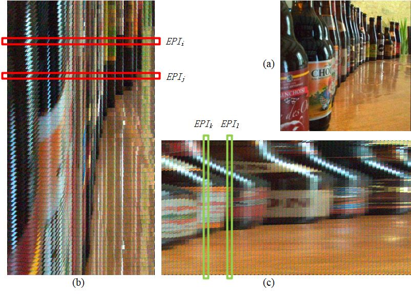
corresponding row is numbers
a central view in theimage
central and (b) isimage.
view part ofIna
horizontal
that case, we EPI synthetic
will image. EPI
get a horizontal EPI i and EPIj selected
synthetic in Figure 3bas
image abbreviated represent
EPIh forEPI the images
whole
corresponding
scene. to rowsan
Figure 3 shows i and j in the
example incentral
which view(a) is image,
a central respectively.
view imageThese EPIs
and (b) is similar
part of toa
EPI are
horizontal
i stitched from top to bottom to form a horizontal EPI
EPI synthetic image. EPIi and EPIj selected in Figure 3b represent EPI images synthetic image. It should be
emphasized that
corresponding to Figure
rows i and 3b isj only
in the a part
centralof the
view vertical
image,clipping of the These
respectively. wholeEPIsEPIhsimilar
so that
the texture structure of the EPIh can be presented at a large
to EPIi are stitched from top to bottom to form a horizontal EPI synthetic image. It should display scale.
Similarly, in
be emphasized thatformula
Figure (2),3b is if the
onlycoordinates
a part of the u and s remain
vertical clippingunchanged,
of the whole but theEPIhcoor-
so
dinates
that v and t structure
the texture change, we willEPIh
of the obtain cananbeEPI corresponding
presented at a large to display
a column of pixels in the
scale.
central view image. Then EPIs of each column in the central view image can be stitched
into a vertical EPI synthetic image (EPIv). Figure 3c is part of a vertical EPI synthetic image,
where the frames of EPIk and EPIl represent EPI images corresponding to columns k and l
in the central view image, respectively.
It can be seen from the above synthesis process that the EPI synthetic images not
only have local linear texture contained depth information but also integrate the spatial
association information of the row or column in the central view image. Therefore, we use
EPIh and EPIv as inputs of the deep neural network to improve feature extraction. Figure 3
illustrates some examples of these input images.Sensors 2021, 21, 6061 6 of 17
Sensors 2021, 21, x FOR PEER REVIEW 6 of 18
Figure 3.
Figure Examples of
3. Examples of input
input images.
images. (a)
(a)isisaacentral
centralview,
view,(b) is is
(b) a horizontal EPIEPI
a horizontal synthetic image,
synthetic (c) is
image, (c)a is
vertical EPI synthetic
a vertical EPI syn-
image.
thetic image.
4. Network Architecture
Similarly, in formula (2), if the coordinates u and s remain unchanged, but the coor-
dinatesOur deept change,
v and neural network
we will designed
obtain an for
EPIdepth estimationtoisadescribed
corresponding column ofinpixels
this section.
in the
We first state the overall design ideas and outline the network architecture,
central view image. Then EPIs of each column in the central view image can be stitched followed by
twoastructural
into vertical EPI details of ourimage
synthetic network, namely
(EPIv). Figure multi-stream
3c is part ofinputs andEPI
a vertical skipconnections.
synthetic im-
Finally, we introduce the loss function used in training the network.
age, where the frames of EPIk and EPIl represent EPI images corresponding to columns k
and l in the central view image, respectively.
4.1. General Framework
It can be seen from the above synthesis process that the EPI synthetic images not only
have We formulate
local depthcontained
linear texture estimationdepth
from the light fieldbut
information as aalso
spatially densethe
integrate prediction task,
spatial asso-
and design a deep convolution neural network (ESTNet) to predict
ciation information of the row or column in the central view image. Therefore, we use the depth of each pixel
in theand
EPIh central
EPIvview image.
as inputs of the deep neural network to improve feature extraction. Figure
In general, the proposed model is a convolutional network with multi-stream inputs
3 illustrates some examples of these input images.
and some skip-connections shown in Figure 4. In essence, our network is a two-stage
4.network.
NetworkThe first stage conducts a downsampling task, and the second stage performs
Architecture
an upsampling job. The downsampling part encodes input images in a lower dimension-
ality,Our deep
while theneural network
upsampling designed
part for depth
is designed estimation
to decode featureis maps
described in this section.
and produce dense
We first state the overall
predictions of each pixel. design ideas and outline the network architecture, followed by
two structural details of our
In the downsampling network,
stage, namely multi-stream
a multi-stream architecture is inputs andtoskipconnections.
utilized learn the geome-
Finally, we introduce the loss function used in training the network.
try information of the light field. The main idea behind the multi-stream architecture is
to receive different inputs from light-field data and extract and fuse their features. Three
4.1. General
streams areFramework
designed with the respective input of the horizontal EPI synthetic image (EPIh),
We formulate
the central view imagedepth estimation
(CV), and thefrom the EPI
vertical light field as image
synthetic a spatially dense
(EPIv). prediction
Different from
task,
EPInetand[5],
design
EPIhaand deep convolution
EPIv neural
are fed with EPInetwork
synthetic (ESTNet)
images to predict
rather thethe
than depth
stackofof
each
the
pixel in the central
sub-aperture images view image.
in one direction. CNN is used to encode features in each stream. Then
In general,
the outputs the proposed
of these streams aremodel is a convolutional
concatenated for further network
encodingwithofmulti-stream
features. inputs
and some skip-connections shown in Figure 4. In essence, our network is a two-stage net-
work. The first stage conducts a downsampling task, and the second stage performs an
upsampling job. The downsampling part encodes input images in a lower dimensionality,Sensors 2021, 21, x FOR PEER REVIEW 7 of 18
Sensors 2021, 21, 6061 7 of 17
while the upsampling part is designed to decode feature maps and produce dense predic-
tions of each pixel.
Figure
Figure4.
4.The
Thearchitecture
architectureof
ofESTNet.
ESTNet.
In
Inthe
thedownsampling
upsampling stage, stage,thea multi-stream
transposed convolutionarchitecturelayer is utilized
is usedtoaslearn the geom-
the core of the
etry information
decoding moduleoftothe light field.
improve The mainofidea
the resolution behind map.
the feature the multi-stream architecture be-
Besides, the connections is
to receive
tween different
modules with inputs
the same fromresolution
light-fieldindata the and extract andstage,
downsampling fuse their features.
and the Three
upsampling
streams
stage areare designed to
established with
fusethetherespective
lower texture input of the horizontal
information EPI synthetic
and the upper semanticimageinfor-
(EPIh),
mation.the Forcentral
the sake view of image (CV), and the
the single-channel verticalmap
disparity EPI synthetic
computation,image a 1(EPIv). Different
× 1 convolution
from
layerEPInet
is added [5],atEPIh
the end andof EPIv
the are fed with EPI synthetic images rather than the stack of
network.
the sub-aperture images in one direction. CNN is used to encode features in each stream.
4.2. Multi-Stream
Then the outputs of Architecture
these streams are concatenated for further encoding of features.
In
Asthe upsampling
shown in Figure stage,
4, ourthemodeltransposed
has three convolution layer is used
feature extraction as the
streams: core
ST1, of and
ST2, the
decoding
ST3, which module
are fedtowith improve
EPIh,the CV,resolution
and EPIv, of the feature map. Besides, the connections
respectively.
between Themodules
stream ofwith ST1 theis composed
same resolution of fourin blocks with similar structures.
the downsampling stage, andEach block is
the upsam-
a stack of convolutional layers: the first convolutional
pling stage are established to fuse the lower texture information and the upper semantic layer is followed by activation of
ReLU, a batch
information. Fornormalization
the sake of the (BN) operation isdisparity
single-channel executedmap aftercomputation, a 1 × 1 con-
the second convolutional
layer andlayer
volution provides
is addedinput atfortheaend
ReLU of activation,
the network. and the end of each block is a max-pooling
layer. The block structures in ST2 and ST3 are the same as those in ST1. In addition, ST3
contains
4.2. the same
Multi-Stream number of blocks as ST1, and ST2 has only three blocks.
Architecture
Now we discuss
As shown in Figure the 4,size of model
our input imageshas three for the threeextraction
feature streams. Suppose
streams:the ST1,dimensions
ST2, and
of the light field are
ST3, which are fed witharEPIh, ( N , N , N
ac CV, , N
sr and , N
sc EPIv,
ch ) , where N ar
respectively. , N ac are angular resolution in a row
and The a column direction, respectively;
stream of ST1 is composed of four N , N
sr blocks
sc indicate space resolution in
with similar structures. Each block a row andis aa
column
stack direction, respectively;
of convolutional layers: theNfirst ch represents
convolutional the number
layer isoffollowed
channelsbyinactivation
a light-fieldof
image. EPIh generated from light-field data has the dimension of ( Nac × Nsr , Nsc , Nch ),
ReLU, a batch normalization (BN) operation is executed after the second convolutional
the dimension of EPIv is ( N , Nar × Nsc , Nch ), and the size of CV is ( Nsr , Nsc , Nch ). For
layer and provides input for asrReLU activation, and the end of each block is a max-pooling
example, the images in Figure 3 were generated from the (9,9,381,381,3) dimensional
layer. The block structures in ST2 and ST3 are the same as those in ST1. In addition, ST3
light-field data collected by the Lytro camera. The resolution of the central view image
contains the same number of blocks as ST1, and ST2 has only three blocks.
(Figure 3a) is 381 × 381, and the resolution of EPIh should be 3429 × 381. However, Figure
Now we discuss the size of input images for the three streams. Suppose the dimen-
3b is only a part of EPIh, and its resolution is 1450 × 381.
sions of the light field are ( N ar , N ac , N sr , N sc , N ch ) , where N ar , N ac are angular resolution
As mentioned above, the input images in the three streams have different dimensions.
in a row and
However, thea column
output of direction,
each streamrespectively;
should reach N sr , N
the indicate
sc same space resolution
resolution in a row
for concatenation
and a columnTherefore,
processing. direction,the parameters,Nsuch
respectively; ch represents
as the size theandnumber of channels
the stride in a light-
for convolutional
kernelimage.
field or max pooling, should be setfrom
EPIh generated reasonably.
light-field data has the dimension of
( N ac ×InNthesr , N sc , N ch ) , the dimension of EPIv is ( N sr , N ar × N sc , N ch ) , and the size of CV is
first block of the ST1 stream, as shown in Table 1, the first convolutional layer
filters the ( Nac × Nsr , Nsc , Nch )-dimensional EPIh with 10 kernels of size (3,3) and a stride
( N sr , N sc , N ch ) . For example, the images in Figure 3 were generated from the (9,9,381,381,3)
of 1 pixel. The second convolutional layer also has 10 kernels of size (3,3) and 1-pixel stride,
dimensional
followed by batch light-field data collected
normalization (BN) layerby theand Lytro
ReLU camera. The resolution
activation. The end ofof thethe central
first block
is spatial pooling carried out by the max-pooling layer. Max-pooling is performed over a
(9,1) pixel window, with stride (9,1). The first block of the ST3 stream is of similar structure
as ST10 s first block, but ST30 s max-pooling stride is (1,9).Sensors 2021, 21, 6061 8 of 17
Table 1. The first block structure in ST1 stream.
Layer Type Output Shape Parameters
Kernel_size = (3,3), stride = 1,
ST1_g1c1 Conv2D (None,4608,512,10)
filter_num = 10
ST1_g1r1 Activation (None,4608,512,10)
Kernel_size = (3,3), stride = 1,
ST1_g1c2 Conv2D (None,4608,512,10)
filter_num = 10
Batch
ST1_g1BN (None,4608,512,10)
Normalization
ST1_g1r2 Activation (None,4608,512,10)
ST1_g1p Max Pooling (None,512,512,10) Pool_size = (1,9)
After the first block processing of the ST1 stream, its output resolution is consistent
with that of the CV image. The same is true for the first block of the ST3 stream. Therefore,
the identical layer structure is designed for the remaining three blocks in ST1 and ST3
streams and the blocks in ST2 stream. In these blocks, all the convolutional layers have
kernel size of (3,3) and stride of 1 pixel, and a Max pooling layer use (2,2) window to slide
with stride 2. The convolutional layers in one block have the same number of filters and
the exact size of feature maps. However, from one block to the next, the feature map size is
halved; the number of filters is doubled to preserve the time complexity per layer.
After the feature extraction of the three streams, we cascade their output results
and then employ three blocks to extract features further. These blocks are shown in the
gray box in Figure 4, where each block is composed of two Conv + ReLU layers, one
Conv + BN + ReLU layer, and one max pooling layer.
After the above encoding stage of feature extraction, the network enters an expansive
path that decodes the feature maps. This stage of the network consists of six blocks which
are divided into two types. The first type block includes one transposed convolution layer,
two Conv + ReLU layers, and one Conv + BN + ReLU layer. Table 2 lists the parameters
of the first type block. Compared with the first type block, the second type block adds a
cascade layer to realize skip-connections and reduce a Conv + ReLU layer. Finally, we use
a 1 × 1 convolutional layer to get the disparity map.
Table 2. The first block structure in the decoding stage.
Layer Type Output Shape Parameters
Kernel_size = (2,2), stride = (2,2),
D_dec_1 Conv2DTranspose (None,64,64,80)
filter_num = 80
D_c1_1 Conv2D (None,64,64,80) Kernel_size = (2,2), stride = (2,2)
D_relu1_1 Activation (None,64,64,80)
D_c2_1 Conv2D (None,64,64,80) Kernel_size = (2,2), stride = (2,2)
D_relu2_1 Activation (None,64,64,80)
D_c3_1 Conv2D (None,64,64,80) Kernel_size = (2,2), stride = (2,2)
D_BN1_1 Batch Normalization (None,64,64,80)
D_relu3_1 Activation (None,64,64,80)
4.3. Skip Connections
Compared with high-level feature maps, shallow features have smaller receptive
fields and therefore contain less semantic information, but the image details are preserved
better [26]. Since depth estimation requires both accurate location information and precise
category prediction, fusing shallow and high-level feature maps is a good way to improve
depth estimation accuracy. Therefore, the proposed model utilizes skip-connections to
retain shallow detailed information from the encoder directly.
Skip-connections connect neurons in non-adjacent layers in a neural network. As
shown in Figure 4, dotted lines indicate skip-connections. With those skip-connections in aSensors 2021, 21, 6061 9 of 17
concatenation fashion, local features can be transferred directly from a block of the encoder
to the corresponding block of the decoder.
In Figure 4, CC1, CC2, and CC3 are the three skip-connections proposed in this
paper. In order to analyze the impact of the number of skip-connections on our network
performance, we compared the experimental results when adding CC4 and CC5 in the
experimental section. The shallow feature map is directly connected to the deep feature
map, which is essentially a cascade operation, so it is necessary to ensure that the resolution
of the two connected feature maps is equal. In theory, skip-connections can be established
for blocks with the same resolution in the two stages, but the experiment shows that three
skip-connections can achieve better results.
4.4. Loss Function
The intuitive meaning of the loss function is obvious: the worse the performance of
the model, the greater the loss, so the value of the corresponding loss function should be
larger. When training a network model, the gradient of the loss function is the basis of
updating network parameters. Ideally, the large value of the loss function indicates that
the model does not perform well, and the gradient of the loss function should be large to
update the model parameters quickly. Therefore, the selection of loss function affects the
training and performance of the model.
We try to train the proposed network (ESTNet) with the loss function of log-cosh.
Log-cosh is calculated by the logarithm of hyperbolic cosine of prediction error, as shown
p
in Formula (5), where yi and yi refer to the ground-truth value and the prediction value
respectively, and the subscript i represents the pixel index.
n
∑ log(cosh(yi
p
L(y, y p ) = − yi )) (5)
i =1
The loss function of log-cosh is usually applied to regression problems, and its central
part log(cosh( x )) has the following characteristics: if the value of x is small, it is approx-
imately equal to x2 /2, and while x is large, it is close to (| x | − log(2)). This means that
log-cosh works much like mean square error (MSE), but is not easily affected by outliers.
5. Experimental Results
5.1. Experimental Setup
5.1.1. Dataset
Our model training is carried out on HCI Benchmark, and the evaluation is respec-
tively conducted on HCI Benchmark [27] and the real light field dataset [28].
HCI benchmark has 28 scenes, each with 9 × 9 angular and 512 × 512 spatial resolu-
tions. This benchmark is designed to include issues that are particularly challenging for
the depth estimation procedure: occlusion of the boundaries, presence of structures, low
textures, smooth surfaces, and camera noise. The scenes were created with Blender using
the internal renderer for the stratified scenes and the Cycles renderer for the photorealistic
scenes. The light field images are set up in a way such that all cameras are shifted towards a
common focal plane while keeping the optical axes parallel. Most scene content lies within
a range of −1.5 px and 1.5 px, though disparities on some scenes are up to 3 px. For each
scene, HCI provides 8-bit light fields (9 × 9 × 512 × 512 × 3), camera parameters, and
disparity ranges. For the stratified and training scenes, the benchmark further includes
evaluation masks and 16bit ground truth disparity maps in two resolutions (512 × 512 px
and 5120 × 5120 px).
The real light field dataset provided by Mousnier et al. [28] is used for testing. The
dataset contains 30 groups of Lytro camera data, including 25 groups of indoor and outdoor
scenes, three groups of motion blur, one group of long-time exposure, and one group of
plane photography. The last three kinds of light-field images are not in the evaluationSensors 2021, 21, 6061 10 of 17
scope of the proposed method. This experiment mainly tests 25 light-field images of indoor
and outdoor scenes.
5.1.2. Experimental Scheme
The proposed network model is implemented using Keras with Tensorflow as the
backend. Our experiment is conducted on hardware configured with Intel Xeon E5-2650
CPU, 64GB memory, and an NVIDIA Quadro K5200 GPU graphics card.
We use 16 scenes in the additional module of the HCI dataset for network training
and 12 scenes in the structured, test, and training modules for network evaluation. In order
to ensure that there are enough training images, we augment data by rotating light-field
images to 90◦ , 180◦ , and 270◦ and flipping them. For the sake of reducing the memory
consumption during training the network, the input of the network is a sub-image with
only 64 × 64 resolution randomly selected from the 512 × 512 resolution image. Moreover,
when preparing the network inputs, we do not rotate the entire 4D light field to generate
a batch of enhanced sample data by slicing the new light field. Instead, we calculate a
batch of enhanced samples through the designed algorithm, keeping the entire light-field
data unchanged. Through the above measures, the number of training images is up to one
million times the number of scenes, ensuring the sample diversity for network input.
We conduct a series of comparative experiments on HCI and real light-field datasets
to evaluate our algorithm’s performance and verify the validity of the multi-stream and
skip-connection network structure.
5.2. Evaluation Metrics
The hierarchical sense of the depth map, especially the evaluation of the object bound-
ary, is of more concern. In our experiment, MSE and BadPix are selected as the evaluation
metrics of algorithm performance analysis. These two metrics are described in refer-
ence [27] and are used by many current relevant methods. For the sake of clarity, we report
this as follows.
Given an estimated disparity map d, the ground truth disparity map gt and an
evaluation mask M, MSE is quantified as
2
∑ x∈ M (d( x ) − gt( x ))
MSE M = × 100 (6)
| M|
And BadPix is formulated as
|{ x ∈ M : |d( x ) − gt( x )| > t}|
BadPix M (t) = (7)
| M|
In (7), t is a disparity error threshold, usually set to one value of 0.01, 0.03, and 0.07.
5.3. Ablation Studies
5.3.1. Multi-Stream Architecture
To verify the effectiveness of the proposed multi-stream architecture, we cut down
the network input streams and conduct experiments to evaluate the performance of single-
stream, double-stream, and three-stream architecture, respectively. Figure 4 shows a
three-stream network. In this network, deleting ST1 or ST3 leads to a double-stream
network; a single-stream network is obtained if both ST1 and ST3 are deleted.
For the above networks with different structures, we train each network on the same
dataset and keep the hyperparameters such as batch and epoch consistent. Then, each
network is tested on the stratified and training groups in the HCI benchmark. According
to the test results, Table 3 lists the average values of computational time, RMS, and BadPix
in eight scenes of the HCI benchmark.Sensors 2021, 21, 6061 11 of 17
Table 3. Performance comparison of networks with the different number of input streams.
Computational Time MSE BadPix(0.07)
Type
(Avg. Units: s) (Avg.) (Avg.)
ST1 0.1914 6.72 12.85
ST2 0.1905 10.04 18.93
ST3 0.1914 6.75 12.87
ST1 + ST2 0.2235 4.48 9.32
ST2 + ST3 0.2235 4.51 9.41
ST1 + ST2 + ST3 0.2314 1.65 3.86
It can be seen from Table 3 that the network with three-stream architecture achieves the
best effect, while the single-stream network is the worst. In the training of the single-stream
network, the loss function reaches the expected threshold value quickly. However, when
the network is applied to the test scene, the estimating depth at the object boundary is not
ideal. This phenomenon may be because the network parameters are relatively small, and
the EPI texture information is not fully utilized.
5.3.2. Skip-Connection Architecture
In order to verify the structure of skip-connections, we designed four groups of
experiments on four kinds of network, including no skip-connection (N-S0), one skip con-
nection (N-S1), three skip-connections (N-S3), and five skip-connections (N-S5). Referring
to Figure 4, we describe the structure of the four networks as follows. N-S0 network means
that all skip-connections of CC1, CC2, CC3, CC4 and CC5 are deleted; if only CC1 is re-
tained and the other skip-connections are deleted, N-S1 network is obtained; N-S3 network
includes CC1, CC2, CC3, but not CC4 and CC5; N-S5 network includes all skip-connections
in the figure.
Similar to the experimental analysis of multi-stream design, the above four networks
(N-S0, N-S1, N-S2, N-S3, N-S4) are trained and tested on the HCI benchmark, respectively.
Table 4 shows the evaluation results of each network regarding MSE and BadPix. As those
data in Table 4 revealed, with the increase of skip-connections, the performance gradually
improves. However, compared with the N-S3 network, the MSE of the N-S4 network is
only slightly improved, but the BadPix is unchanged.
Table 4. Performance comparison of networks with the different number of skip-connections.
MSE BadPix(0.07)
Type
(Avg.) (Avg.)
N-S0 8.59 10.25
N-S1 3.64 6.85
N-S2 2.85 5.02
N-S3 1.65 3.86
N-S4 1.60 3.81
N-S5 1.60 3.80
After the ablation study, we determine our network, including three input streams of
ST1, ST2, ST3, and three skip-connections of CC1, CC2, and CC3 (see Figure 4).
5.4. Comparison to State-of-the-Art
5.4.1. Quantitative Comparison
In this subsection, the performance of the proposed model is evaluated using a syn-
thetic light-field dataset, namely the HCI dataset mentioned above. We compared our
ESTNet with the following state-of-the-art models: EPInet [5], EPI-refocus-net [23], Fun-
sionNet [24], and VommaNet [25]. These networks are trained and evaluated quantitatively
based on the scenes and the ground truth values of the HCI dataset.Sensors 2021, 21, 6061 12 of 17
Figure 5 shows the MSE results of each network in some scenes of HCI. Each row
in the figure corresponds to a scene in the HCI dataset. The central view images of these
scenes are arranged in the first column. The scene names are cotton, dino, pyramids, and
stripes, from top to bottom. The other columns are the results of each network. The number
above each image is the MSE metric value of the corresponding network in the scene. At
the end of each line is the color ruler of the image. The smaller the deviation between
the estimated depth and the true value of each pixel position in the image, the lighter the
pixel’s color. Furthermore, the greater the positive deviation, the darker the red, the greater
the negative deviation, and the darker the blue.
Figure 6 shows the Badpix index test results of each network. The layout of the figure
is similar to that of Figure 5, but the color distribution of pixels is slightly different. When
the Badpix error is small, the pixel is green, but when the Badpix error increases, the pixel
changes from green to red.
It can be seen from Figure 5; Figure 6 that ESTNet proposed by this paper has achieved
reasonable performance. Although our network is not the best in every scene, it has reached
a better average level (see Table 5). As shown in Figure 5, the results of ESTNet show that
the color in the beard of the cotton scene, the wall of the scene, the ball of the pyramids
scene, and the stripe of the stripes scene tends to be white, indicating that the MSE index
of these regions is small. Therefore, our network has a relatively excellent MSE index in
Sensors 2021, 21, x FOR PEER REVIEW 13 of 18
the homogeneous region of the scene, which proves that our network can improve the
accuracy of depth estimation by constructing EPI synthetic texture images.
Figure5.5.Examples
Figure Examplesof
ofMSE
MSEresults
resultsfor
foreach
eachnetwork.
network.
Figure 6 shows the Badpix index test results of each network. The layout of the figure
is similar to that of Figure 5, but the color distribution of pixels is slightly different. When
the Badpix error is small, the pixel is green, but when the Badpix error increases, the pixel
changes from green to red.
It can be seen from Figures 5 and 6 that ESTNet proposed by this paper has achieved
reasonable performance. Although our network is not the best in every scene, it has
reached a better average level (see Table 5). As shown in Figure 5, the results of ESTNet
show that the color in the beard of the cotton scene, the wall of the scene, the ball of the
pyramids scene, and the stripe of the stripes scene tends to be white, indicating that theSensors 2021, 21, 6061 13 of 17
Sensors 2021, 21, x FOR PEER REVIEW 14 of 18
Figure 6.
Figure 6. Examples
Examples of
of BadPix
BadPix results
results for
for each
each network.
network.
Table5.5. Performance
Table Performance comparison
comparisonof
ofcurrent
currentpopular
popularneural
neuralnetworks.
networks.
Computational
Computational Time MSE MSE BadPix(0.07)
BadPix(0.07)
Methods
Methods
(Avg. Units:
Units: s)
Time (Avg. s) (Avg.) (Avg.) (Avg.)
(Avg.)
ESTNet
ESTNet 0.2314
0.2314 1.652 1.652 3.857
3.857
EPINet_9 ××99[5]
EPINet_9 [5] 2.041
2.041 2.521 2.521 5.406
5.406
EPI-refocus-net [23] 303.757 3.454 5.029
EPI-refocus-net [23] 303.757 3.454 5.029
FusionNet [24] 303.507 3.465 4.674
FusionNet [24]
Vommanet_9 × 9 [25] 303.507
1.882 3.465 2.556 4.674
10.848
Vommanet_9 × 9 [25] 1.882 2.556 10.848
As shown in Figure 5, the results of the current light field depth estimation methods
As shown in Figure 5, the results of the current light field depth estimation methods
based on neural networks generally exist in the case of relatively large MSE values at the
based on neural networks generally exist in the case of relatively large MSE values at the
object boundary. However, as seen in the Badpix index of Figure 6, the performance of our
object boundary. However, as seen in the Badpix index of Figure 6, the performance of
method is fairly good at the occlusion boundary. It shows that the depth estimation error
our method is fairly good at the occlusion boundary. It shows that the depth estimation
of object boundary is larger than that of the internal area, but is still in the acceptable range
error of object boundary is larger than that of the internal area, but is still in the acceptable
(less than 0.07). Therefore, our network has some advantages in occlusion processing.
range (less than 0.07). Therefore, our network has some advantages in occlusion
Table 5 lists the average MSE, average Badpix, and average computational time of
processing.
each network when tested on the HCI dataset. These results come from the reports of each
Table
network 5 lists Although
author. the average in MSE, average of
the examples Badpix,
Figureand average6, computational
5; Figure our ESTNet does timenot
of
each network when tested on the HCI dataset. These results come from the
have the best metrics in every scene, it achieves the best average MSE and average BadPixreports of each
networkas
metrics, author.
shownAlthough
in Table 5.in the examples of Figures 5 and 6, our ESTNet does not have
the best metrics in every scene,
The hardware platforms it achieves
of each networkthe
arebest average
different (seeMSE
Tableand average
6), so BadPix
the computa-
metrics, as shown in Table 5.
tional time cannot be strictly compared, but the difference in computational time of each
The can
network hardware platforms
still be analyzed of eachtonetwork
according are different
the calculation power of(see Table 6), Among
the platform. so the
computational time cannot be strictly compared, but the difference in computational
K5200, TITAN X and 1080Ti, 1080Ti has the strongest computing power, but a single 1080Ti time
of each network can still be analyzed according to the calculation power
is less than two TITAN X and K5200 has the weakest computing power. Under the weakest of the platform.
Among
GPU K5200, TITAN
computing power,Xour and 1080Ti,achieves
ESTNet 1080Ti has the strongest
the shortest computing
computing time, power, but a
even several
single 1080Ti is less than two TITAN X and K5200 has the weakest computing power.Sensors 2021, 21, x FOR PEER REVIEW 15 of 18
Sensors 2021, 21, 6061 14 of 17
weakest GPU computing power, our ESTNet achieves the shortest computing time, even
several
orders oforders of magnitude
magnitude lower
lower than than EPI-refocus-net
EPI-refocus-net and FusionNet.
and FusionNet. AlthoughAlthough the
the measure-
measurement
ment of MSE and of MSE andofBadPix
BadPix of our
our ESTNet ESTNet to
is inferior is that
inferior to thatinof
of EPINet EPINet
some in some
scenes, it has
scenes,
apparentit has apparentinadvantages
advantages in computational
computational time. To sumtime. To sumcan
up, ESTNet up,balance
ESTNetthe
canaccuracy
balance
of depth
the estimation
accuracy of depthand computational
estimation time.
and computational time.
Table
Table 6. Runtime environment of current popular neural networks.
Methods
Methods Runtime
RuntimeEnvironment
Environment
Window 10 64bit, Intel Xeon E5-2650
Window 10 64bit, Intel Xeon E5-2650 @2.3GHz,
@2.3GHz,64GB
64GB RAM,
RAM,
ESTNet
ESTNet
NVIDIA
NVIDIA Quadro K5200
Quadro K5200GPU
GPU
EPINet_9
EPINet_9 × 9×[5]
9 [5] Window10
Window10 64bit,
64bit, i7-7700
i7-7700 @3.6GHz,
@3.6GHz, 32GBRAM,
32GB RAM,1080Ti
1080Ti
EPI-refocus-net
EPI-refocus-net [23] [23] ntel Core i7-4720HQ 2.60GHz + Two TITAN
ntel Core i7-4720HQ 2.60GHz + Two TITAN X GPUs X GPUs
FusionNet [24] Intel Core i7-4720HQ 2.60GHz + Two TITAN X GPUs
FusionNet [24]
Vommanet_9 × 9 [25] Intel
UbuntuCore i7-4720HQ
16.04 2.60GHz
64bit, E5-2603 + Two64GB
v4 @1.7GHz TITAN X GPUs
RAM, GTX 1080Ti
Vommanet_9 × 9 [25] Ubuntu 16.04 64bit, E5-2603 v4 @1.7GHz 64GB RAM, GTX 1080Ti
5.4.2. Qualitative Comparison
5.4.2. Qualitative Comparison
In this section, the experiments are carried out on the real light-field dataset to ver-
In this section, the experiments are carried out on the real light-field dataset to verify
ify our ESTNet performance in the scenes with noise. As mentioned earlier, the Lytro
our ESTNet performance in the scenes with noise. As mentioned earlier, the Lytro camera
camera captured this light field dataset [27], mixed with various imaging noises, but
captured this light
without depth field dataset
ground-truth [27],
value. mixed with
Therefore various
we make imagingcomparisons
qualitative noises, but through
without
depth ground-truth
visual observation. value. Therefore we make qualitative comparisons through visual ob-
servation.
Considering the availability of method code, we choose Tao [7], Jeon [16], Lin [17],
ShinConsidering
[5], and Heberthe [22]
availability
methodsoftomethod code,
compare withweour
choose Tao [7],
ESTNet. Jeon [16],
As shown Lin [17],
in Figure 7,
Shin [5], and Heber [22] methods to compare with our ESTNet. As shown in Figure
taking five scenes in the real light-field dataset as examples, the depth estimation results of7,
taking five scenes
each method in theinreal
are given thelight-field
columns. dataset as examples, the depth estimation results
of each method are given in the columns.
Scenes Ours Tao Jeon Lin Shin Heber
Figure 7. Examples of depth estimation results for each method in the real light field.
Figure 7. Examples of depth estimation results for each method in the real light field.
Among methods of
Among methods ofqualitative
qualitativecomparison
comparisonexperiment,
experiment, Tao
Tao [7],[7],
Jeon Jeon
[16],[16],
andand Lin
Lin [17]
[17] are traditional methods based on energy optimization, while Shin [5], Heber
are traditional methods based on energy optimization, while Shin [5], Heber [22], and ours[22], and
ours are deep
are deep neural
neural network
network methods.
methods. From
From thethe perspective
perspective ofofdepth
depthlevel,
level,ititcan
can bebe seen
seenSensors 2021, 21, 6061 15 of 17
from Figure 7 that the results of the methods based on deep neural networks are generally
better than those of traditional energy optimization methods. The disparity maps of the
traditional methods can only clearly show fewer depth levels. In particular, the results of
the Tao method are fuzzy, and the contour of the object is invisible. On the contrary, the
results of Shin, Heber, and our network can show more depth levels.
The method based on depth neural network generally has insufficient smoothness;
especially, the EPINet results show more noise patches in the flat area. However, the results
of traditional methods are smoother in homogeneous regions because the energy function
used by the traditional method contains the smoothing term.
It is worth mentioning that our network has achieved relatively good depth estimation
results. For instance, in the scene shown in the last row of Figure 7, the sky is inverted at a
little distance by all other methods. But our approach successfully deals with the depth
level of the sky.
These methods use different programming languages and different platforms. Some
methods call on GPU resources, while others only use CPU. Therefore, the computational
time is not comparable and is not listed.
6. Conclusions
In this paper, ESTNet is designed for light-field depth estimation. The idea behind
our design is the principle of epipolar geometry and the texture extraction ability of
a convolutional neural network (CNN). We first analyze the proportional relationship
between the depth information and the slope of the straight line in an EPI, and then
combine EPIs by row or column to generate EPI synthetic images with more linear texture.
The proposed ESTNet network uses multi-stream inputs to receive three kinds of image
with different texture characteristics: horizontal EPI synthetic image (EPIh), central view
image (CV), and vertical EPI synthetic image (EPIv). EPIh and EPIv have more abundant
textures suitable for feature extraction by CNN. ESTNet is an encoding-decoding network.
Convolution and pooling blocks encode features, and then the transposed convolution
blocks decode features to recover depth information. Skip-connections are added between
encoding blocks and decoding blocks to fuse the shallow location information and deep
semantic information. The experimental results show that EPI synthetic images as the
input of CNN are conducive to improving depth estimation performance, and our ESTNet
can better balance the accuracy of depth estimation and computational time.
Since the strides of the first max-pooling layers of ST1 and ST3 in ESTNet are (9,1) and
(1,9), respectively, the limitation of our method is that the number of views used in EPI
synthetic images is fixed to nine. At present, the number of horizontal and vertical views of
most light field cameras is nine or more. If there are more than nine views in the horizontal
or vertical direction, we can select only nine. Therefore, although this method cannot be
adaptive to the number of views, it can estimate depth from light-field data captured by
most plenoptic cameras available.
Author Contributions: Conceptualization, L.H. and X.H.; methodology, L.H. and Z.S.; software, S.Z.;
validation, L.H. and S.Z.; formal analysis, L.H., X.H., Z.S. and S.Z.; investigation, L.H.; resources,
L.H. and S.Z.; data curation, S.Z.; writing—original draft preparation, L.H. and Z.S.; writing—review
and editing, L.H. and X.H.; visualization, S.Z.; supervision, L.H. and X.H.; project administration,
L.H. and S.Z.; funding acquisition, L.H. and X.H. All authors have read and agreed to the published
version of the manuscript.
Funding: This work has been supported by Natural Science Foundation of Nanjing Institute of
Technology (Grant Nos. CKJB201804, ZKJ201906), National Natural Science Foundation of China
(Grant No. 62076122), the Jiangsu Specially-Appointed Professor Program, the Talent Startup project
of NJIT (No. YKJ201982), Science and Technology Innovation Project of Nanjing for Oversea Scientist.
Institutional Review Board Statement: Not applicable.
Informed Consent Statement: Not applicable.You can also read