Elucidating the Life Cycle of Warm-Season Mesoscale Convective Systems in Eastern China from the Himawari-8 Geostationary Satellite - MDPI
←
→
Page content transcription
If your browser does not render page correctly, please read the page content below
remote sensing
Article
Elucidating the Life Cycle of Warm-Season Mesoscale
Convective Systems in Eastern China from the
Himawari-8 Geostationary Satellite
Dandan Chen 1 , Jianping Guo 1, * , Dan Yao 1 , Zhe Feng 2 and Yanluan Lin 3
 1   State Key Laboratory of Severe Weather, Chinese Academy of Meteorological Sciences, Beijing 100081, China;
     dandan.chen@163.com (D.C.); yaod@cma.gov.cn (D.Y.)
 2   Atmospheric Sciences and Global Change Division, Pacific Northwest National Laboratory, Richland,
     Washington, DC 99352, USA; zhe.feng@pnnl.gov
 3   Ministry of Education Key Laboratory for Earth System Modeling, and Department for Earth System Science,
     Tsinghua University, Beijing 100084, China; yanluan@mail.tsinghua.edu.cn
 *   Correspondence: jpguo@cma.gov.cn

 Received: 20 May 2020; Accepted: 15 July 2020; Published: 18 July 2020

 Abstract: The life cycle of mesoscale convective systems (MCSs) in eastern China is yet to be fully
 understood, mainly due to the lack of observations of high spatio-temporal resolution and objective
 methods. Here, we quantitatively analyze the properties of warm-season (from April to September
 of 2016) MCSs during their lifetimes using the Himawari-8 geostationary satellite, combined with
 ground-based radars and gauge measurements. Generally, the occurrence of satellite derived MCSs
 has a noon peak over the land and an early morning peak over the ocean, which is several hours
 earlier than the precipitation peak. The developing and dissipative stages are significantly longer as
 total durations of MCSs increase. Aided by three-dimensional radar mosaics, we find the fraction of
 convective cores over northern China is much lower when compared with those in central United
 States, indicating that the precipitation produced by broad stratiform clouds may be more important
 for northern China. When there exists a large amount of stratiform precipitation, it releases a large
 amount of latent heat and promotes the large-scale circulations, which favors the maintenance of
 MCSs. These findings provide quantitative results about the life cycle of warm-season MCSs in
 eastern China based on multiple data sources and large numbers of samples.

 Keywords: mesoscale convective system (MCS); eastern China; Himawari-8; three-dimensional radar
 mosaics; precipitation

1. Introduction
      Mesoscale convective systems (MCSs) are one of the most impactful weather phenomena on Earth.
MCSs are defined as convective systems with contiguous precipitation over 100 km in at least one
direction [1,2]. More importantly, MCSs contribute significantly to warm-season precipitation, both in
the tropics and mid-latitude regions [3,4].
      The intensity and explicit structures of MCSs are affected by a variety of factors, including low-level
jet streams [5–7], topography [8,9] and large-scale circulation [10,11]. For instance, the topography
significantly affects the life cycle of MCSs over the land by facilitating their ascending motions in early
stages [12]. Large-scale circulation plays a well-recognized role in the development of MCSs as well.
The MCSs in the mid-latitude regions tend to occur most frequently in front of the troughs in the
prevailing westerlies [13]. Low-level jet streams tend to enhance MCS formation and continuation at
the downstream region, due to the increase in atmospheric instability and the advection of warm and
moist air masses [14].

Remote Sens. 2020, 12, 2307; doi:10.3390/rs12142307                         www.mdpi.com/journal/remotesensing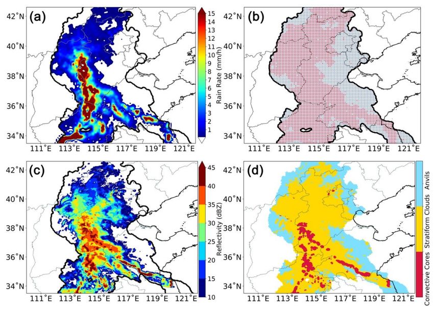
Remote Sens. 2020, 12, 2307                                                                        2 of 22

     Previous studies have attempted to elucidate the life cycle of MCSs, most of which focus on MCSs
in the tropical regions. The earliest studies of MCS life cycle date back to the 1970s and 1980s [15,16],
when the Global Atmospheric Research Program (GARP) Atlantic Tropical Experiment (GATE) [17]
was performed over the tropical Atlantic. The GATE field campaign mainly relied on a wide range of
ship-borne and air-borne measurements to provide primary knowledge of structures and air motion
during different stages of MCSs covering limited periods [18,19]. The advent of geostationary satellites
made it possible to characterize the temporal evolution of MCSs over a much longer period and
larger spatial domain [20–22]. In particular, Pope et al. [23] explored the relationships between
the initial expansion, merging processes, and duration of MCSs from Geostationary Meteorological
Satellite-5. Given that MCSs observed by geostationary satellites may not produce rainfall reaching
the ground surface [2], radar and gauge observations have been widely applied to further verify
satellite derived MCSs [24,25] and reveal their internal structures [26,27]. The precipitation radar
onboard the Tropical Rainfall Measuring Mission (TRMM) and the Global Precipitation Measurement
(GPM) mission are commonly used to investigate the vertical structures of tropical MCSs [28,29]
and mid-latitude MCSs [30]. CALIPSO and Cloudsat can also help to study vertical structures of
MCSs [31]. Combined with information from geostationary satellites, the variations of MCSs in clouds
and precipitation were explicitly revealed during different stages of their lifetimes [30,31].
     Previous efforts to understand MCSs in eastern China mainly focused on the distribution of
MCSs and their interactions with synoptic patterns and topography [32–34]. Currently, knowledge on
the spatiotemporal evolutions of MCSs in eastern China remains deficient and is worthy of further
analyses. Therefore, based on our previous detections and tracking results of MCSs from the Advanced
Himawari Imager (AHI) onboard the Himawari-8 (HW8) satellite [35], the principal goal of this work
was to elucidate the life cycle of MCSs over the eastern China plain, providing cross comparisons of
MCS characteristics to those in the U.S. Great Plains. The Chinese radar network used in this study was
similar to the NEXRAD (Next Generation Weather Radar system) of the U.S. in design, resolution and
distancing, making the radar data and retrieved results comparable. By means of the three-dimensional
(3D) radar mosaics, we gained a better understanding of the convective cores (CCs), stratiform clouds
(SCs), and non-precipitating anvils of MCSs over northern China and variations in their features over
the MCS lifetimes.

2. Data and Methods

2.1. Data and Study Area
     AHI is the most important payload onboard HW8, which was launched by the Japan Meteorological
Agency and is located at 140.7◦ E longitude on the equator [36]. Observations with high spatiotemporal
resolution (from 0.5 to 2 km and 2.5 to 10 min) [37] have been made publicly available since July 2015.
In this study, data from April to September of 2016 as observed by AHI/HW8 were used. To determine
the life cycle of MCSs, we directly applied the tracking results (i.e., trajectories, along with spatial
area, minimum cloud top temperature etc.) at 2 km resolution at 10 min intervals derived from a
recently developed tracking algorithm [35]. The newly developed tracking algorithm combined the
Kalman Filter method with the conventional area overlapping method to capture the motions of
MCSs. When MCSs have larger spatial area or move slowly, their spatial areas on the two consecutive
images have some pixels in common, and then the area overlapping method is used to track the
MCSs. However, for fast-moving MCSs and small MCSs, the area overlapping method does not
work. Therefore, the motions of current MCSs were predicted by the Kalman Filter equations at first.
Secondly, we found the one nearest to the predicted positions among all the MCSs at the next time,
and then matched them with current MCSs. Here, MCS was defined from the geostationary satellite
images, i.e., a convective system with maximum area ≥ 10,000 km2 (region within the isotherms of
brightness temperature of 235 K) and duration ≥ 3 h, which is different from the above-mentioned
definition based on ground precipitation by Houze [19]. Given the large uncertainty associated with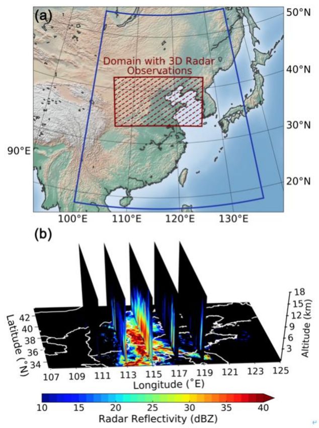
Remote Sens. 2020, 12, 2307                                                                                   3 of 22

clouds as detected from AHI/HW8 over northwestern China, which is largely due to large sensor
zenith angles of AHI [38], this study focused on the temporal evolutions of MCSs over eastern China
(100–136◦ E, 18–54◦ N, bounded by blue lines in Figure 1a) from the perspective of AHI/HW8 and gauge
measurements. For a certain area (regions hatched in red in Figure 1a), we also discuss the life cycle of
internal structures of MCSs with the aid of radar mosaics.

      Figure 1. (a) Region of interest (bounded by blue lines) in eastern China. The area hatched in red refers
      to the domain with three-dimensional (3D) radar observations. (b) The latitude-vertical cross-sections
      of radar reflectivity (shaded colors) merged by the Advanced Regional Prediction System at 1130 UTC
      on 19 July 2016 over northern China, superimposed on the composite reflectivity mosaic.

     Also applied in this research are ground-based 3D radar mosaics and the China Hourly Merged
Precipitation Analysis (CMPA). The 3D radar mosaics used here to identify internal structures of
MCSs were acquired from 21 Doppler radar measurements in northern China. The original radar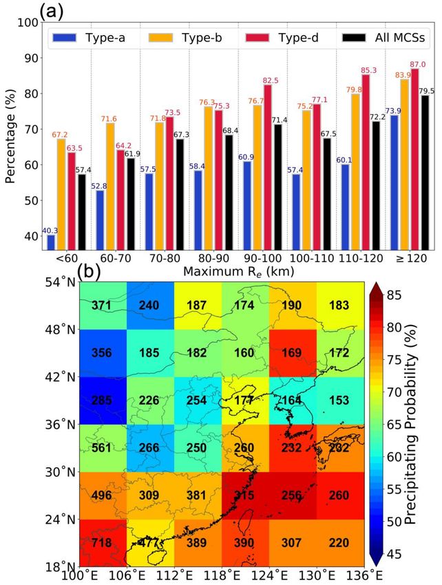
Remote Sens. 2020, 12, 2307                                                                        4 of 22

observations were observed at 11 angles of elevation every 6 min. To make the radar information
much easier to analyze, the preprocessing module of the Advanced Regional Prediction System
(ARPS) [39,40] was used here to interpolate the original observations onto uniform 3D grid points.
This dataset offers observations of echo intensity at 36 levels every 30 min, with a resolution of 2 km
horizontally (in Lambert projection) and 500 m vertically, almost identical to Feng et al. [26]. The 2 km
horizontal resolution of the mosaic product is lower than the 1 km native resolution of the S-band
radar, to avoid potential representative issues induced by the inhomogeneity of the radar observation.
Note that the radial resolution is evenly 1 km, but the tangential resolution is 1◦ , making the actual
grid spacing vary with the distance from the radar. The vertical resolution is a balance of accuracy
and the need for investigation, since the radar only observes the limited levels of specific elevation
angles. Interpolation errors are inevitable, especially in regions close to the mountainous area and in
the vertical direction, but it should not deteriorate the results, which are the best we can get under
current techniques.
      The CMPA is widely used for robust observations of hourly precipitation in eastern China [41],
which assimilates hourly observations from automatic weather stations (primarily over land) with
CMORPH (Climate Prediction Center morphing technique) and can fully cover the region of interest at
a spatial resolution of 0.1◦ .
      To better perform the analysis, the AHI cloud detection results were combined with the radar
mosaic and CMPA data, respectively, using a sampling method based on adjacent pixels. Specifically,
for each grid point in the radar mosaic field, if two or more of the four adjacent pixels around the same
location in the AHI grid were detected within the range of a certain MCS, then the radar echo at this
grid point was considered to be caused by this MCS. The same idea was also applied to the CMPA
field. Figure 1b shows an example of the 3D radar reflectivity mosaic of the study area corresponding
to 1130 UTC on 19 July 2016, acquired using the ARPS.

2.2. Identification of MCS Extent and Internal Structures
      The MCSs observed by AHI/HW8 were roughly determined first based on the isotherms of
brightness temperature (BT) equals to a certain value defined as BTinit , which was then extended
iteratively to BTedge at 1 K step, to include the adjacent anvils of the same MCS and determine the final
range of MCSs. Meanwhile, the iteration was terminated whenever the edge of an MCS at a certain BT
shared common pixel(s) with a neighboring one. This was able to effectively prevent the overlapping
between precipitation regions of the targeted MCS and those associated with others. As such, we
were able to capture the actual range of MCSs and their precipitation with more accuracy. Here, the
thresholds of BTinit and BTedge were chosen as 235 and 250 K, respectively, fairly consistent with
previous studies [42,43]. Further discussions on the associated uncertainties induced by the selection
of threshold values will be given in Section 4.
      Based on the precipitation data from CMPA and AHI/HW8 observations mentioned above, we
further derived the precipitation area collocated with each MCS, as shown in Figure 2a. For instance,
inside the closed isotherms of BTedge , the precipitation produced by a certain MCS is displayed in
Figure 3a. All grid points with a rain rate ≥ 0.1 mm/h on the ground were treated as precipitation
regions associated to the MCS (red dots in Figure 3b), since 0.1 mm/h is the minimum rain rate that can
be detected. Suppose the coverage of the extended MCS (isotherm of BTedge ) is S (in unit of km2 ), the
number of grid points inside the area is Nt , and the number of grid points with rain rate ≥ 0.1 mm/h is
Np . The equivalent radius (Re in units of km) of the MCS is derived as the square root of S/π and the
precipitation ratio is calculated as Np divided by Nt .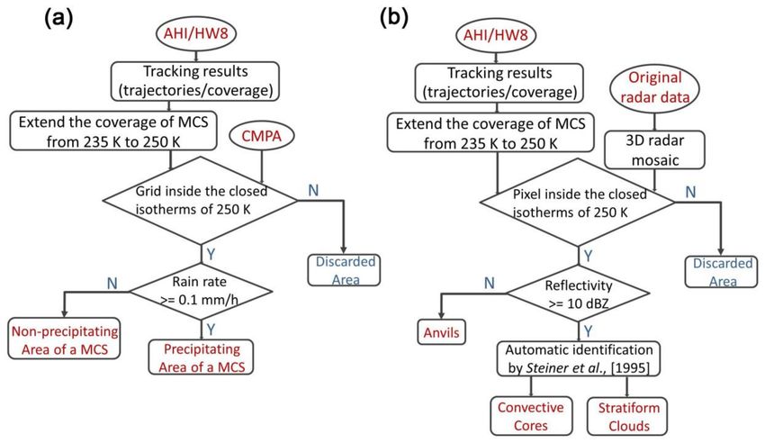
Remote Sens. 2020, 12, 2307                                                                                 5 of 22

      Figure 2. Flow chart showing (a) how to judge precipitating/non-precipitating area of a mesoscale
      convective system (MCS), and (b) how to identify different internal structures (i.e., convective cores,
      stratiform clouds and anvils) of an MCS.

      The flow chart of how to identify different internal structures of MCSs is shown in Figure 2b.
The analysis method is similar to that used by Feng et al. [26] and Feng et al. [27] who jointly analyzed
collocated geostationary satellite and ground-based radar network data. Based on the combination
of radar reflectivity at a selected fixed level (Figure 3c) and cloud observations from AHI/HW8, we
first determined the CCs, SCs, and non-precipitating anvils of each MCS (Figure 3d) to better examine
the internal structures and their variations over the course of an MCS lifetime. To minimize the
likelihood of bright-band contamination, the radar reflectivity at 2–3 km above sea level was generally
chosen when judging the internal structures of MCSs, which was generally below the 0 ◦ C level in
the extratropics [44]. Given that radar observations exhibit significant terrain variations from west to
east, some western parts of the domain have an elevation exceeding 2.5 km, and thus the fixed level of
3 km was used here for judging internal structure of an MCS. As such, both CCs and SCs could be
determined according to an objectively identified method. The CCs were identified based on three
criteria [45]. First, the grid points with radar reflectivity exceeding a given threshold were directly
identified as CCs. In previous studies, a threshold between 40–45 dBZ was generally used. Here, we
chose 40 dBZ based on analyzing the probability density function of radar reflectivity at 3 km above
sea level (the 90th percentile, shown in Figure S1). Secondly, we calculated the background intensity
of each grid by the averaged intensity within 6 km radius centered on it. Then, all the grid points
with echo intensity significantly higher than the background intensity were treated as CCs as well.
Thirdly, if the neighboring grid points around the CCs as judged in the first two steps were within the
appropriate radius centered on CCs (the radius is a function of reflectivity), these grid points were
also identified as CCs. The other grid points with reflectivity higher than or equal to 10 dBZ but not
identified as CCs were determined as SCs. Afterwards, the remaining parts, which were inside the
extent of MCSs but not identified as CCs or SCs, were treated as non-precipitating anvils [26,44].
Remote Sens. 2020, 12, 2307 6 of 22
Figure 3. Schematic diagram showing how to quantify the precipitation and precipitation area produced
by an MCS. The black line in each panel marks the extent of the MCS at 1100 UTC on 19 July 2016
over northern China, with cloud top brightness temperature (BT) less than 250 K. Inside the isotherm
of 250 K, the rain rate is shaded by colors and superimposed on the map in panel (a), while in panel
(b) the red solid (blue hollow) dots are those grid points with (without) precipitation reaching ground,
with a rain rate higher than or equal to (less than) 0.1 mm/h. Panel (c) is same as (a), but shaded by
radar reflectivity at 3 km above sea level, and panel (d) is shaded by different internal structures of an
MCS as derived from reflectivity at 3 km above sea level.
2.3. Determination of MCS Life Stages
With respect to the splitting and merging processes of MCSs, life cycles of the secondary MCS
generation/termination due to splitting/merging processes embedded in the major MCSs are not
complete cycles of classic MCSs. Therefore, the cases mentioned above should be removed from our
samples when used for statistics and compositions of life cycles of classic MCSs, so the following
three types of MCSs were distinguished at first: Type a, secondary MCS generation due to splitting
processes (Figure 4a); Type b, secondary MCS termination due to merging processes (Figure 4b); Type c,
secondary MCS generation initially by splitting processes and then followed by termination due to
merging into other systems (Figure 4c). However, Types a-c only account for secondary MCSs which
do not exhibit entire life cycles, and hence are not considered as our research focus. For MCSs with
entire life cycles, we further analyzed the relative occurrence time of minimum BT and maximum Re
as the peak value of the vertical development and horizontal size of the storm, respectively. Types d-f
correspond to MCSs reaching their maximum vertical development before, after and simultaneously
with their maximum size. According to the definitions proposed in previous studies [28], only Type-d
MCS was considered typical and dominant (i.e., the peak vertical development should be reached in
advance to the peak size) and used in further analyses. It should be noted that the number of samples
in Type e and Type f are much smaller than those in Type d (Table S1), and hence distinguishing them
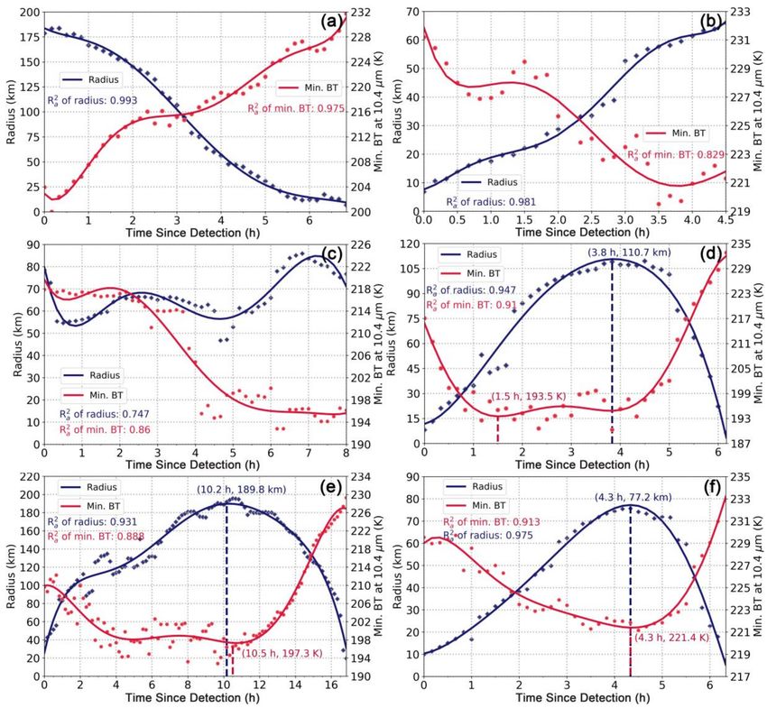
may not affect the reliability of the results.Remote Sens. 2020, 12, 2307 7 of 22
Figure 4. Temporal evolution of minimum BT and equivalent radius (Re ) of six different types of MCS
during their normalized lifetime: (a) MCSs with a large size when they are first detected, followed
by continuously shrinking sizes and decreasing cloud tops; (b) MCSs with small size when they are
first detected, followed by continuously enlarging sizes and rising cloud tops; (c) MCSs with sizes that
do not change much during their lifetime except for the rising cloud tops. (d)–(f) denote the MCSs
with entire lifecycles, differing by the time when the minimum BT occurs being ahead of (d), being lag
behind (e), and at the same time as the time when the maximum Re occurs (f). Additionally, R2a refers
to the coefficient of determination, measuring the goodness of fit of the sixth-order polynomial fitting.
For each MCS of interest, we further derived the fitting curves of its vertical development and
size as a function of time (Figure 4). Some of the MCSs have large sample dispersions in the time series
of minimum BT and Re observations (e.g., red scatters in Figure 4b), which may include noises but
may also contain important features in the MCS lifetime. To extract the main features from noises, we
chose sixth-order polynomial fits, following a previous study [28], for the variations in both minimum
BT and Re in MCSs over their lifetime. To measure the goodness of fit of the polynomial fitting, we
calculated the coefficient of determination R2a as follows:
Suppose there are some observations as y1 , y2 , y3 , . . . , yN , and the corresponding fitting values
are f1 , f2 , f3 , . . . , fN . The average of the observations is calculated as:
N
1 X
y= yi (1)
N
i=1Remote Sens. 2020, 12, 2307 8 of 22
The total sum of squares (TSS) is:
N
X 2
TSS = yi − y (2)
i=1
The residual sum of squares (RES) is:
N
X 2
RES = yi − fi (3)
i=1
It follows that the coefficient of determination R2a is expressed as:
RES
R2a = 1 − (4)
TSS
Here, only those cases with relatively small sample dispersions (R2a ≥ 0.6) were used for statistics.
Given that higher order polynomial fits may result in overfitting issues, while lower order polynomial
fits may not match the observations very well, the fourth-order polynomials were also tested in
this study, and the fitting results are not quite different from those using sixth-order polynomial.
The associated uncertainties induced in the algorithm will be discussed in Section 4.
Consequently, the life stages can be divided with confidence. The developing stage is defined
as the period from the time from when the MCS is first detected to the time when the MCS reaches
the minimum BT. The dissipative stage is the period after the time when the maximum Re occurs.
The period between the developing and dissipative stages corresponds to the mature stage of the MCS.
3. Results
3.1. Precipitation Probability of MCSs from AHI/HW8
Certain cloud systems tracked by geostationary satellite data may not be associated with deep
convective clouds that produce measurable precipitation reaching ground, because the Infrared-only
tracking method may artificially pick up segments of persistent non-precipitating upper-level clouds [2].
One common example is the large non-precipitating upper-level clouds associated with mid-latitude
synoptic disturbances (e.g., cyclones). Those clouds appear with cold cloud-top temperature and may
last for several hours, but do not produce considerable precipitation reaching the ground. According
to the common definition of MCSs, we use additional precipitation observations within the tracked
systems, to identify true MCSs in this study. That is to say, the type of cold clouds mentioned
above as observed by AHI only satisfies our criteria on BT, size, and duration, but does not satisfy
the precipitation requirements. Therefore, those inactive cold clouds should not be treated as true
MCSs [46]. However, the convective clouds embedded in the synoptic scale systems, which produce
enough precipitation reaching the ground, are regarded as true MCSs and used for further analysis in
this study.
The precipitation criteria added as additional constraints to identify MCSs are defined as follows:
the MCS episode must have at least two consecutive hours with precipitation (i.e., the accumulated
precipitation over all grid points within the tracked cloud system at each time > 0.1 mm), and the
precipitation ratio (i.e., the number of grid points with rain rate ≥ 0.1 mm/h divided by the total number
of grid points within the tracked cloud system) during each hour should be no less than 20%. In this
way, the precipitation probability of various types of potential MCSs can be derived as a function of the
maximum Re during the course of its life cycle (Figure 5a). In general, most potential MCSs detected
by AHI have a 50% to 90% chance of producing precipitation, irrespective of the MCS size or type.
The larger the potential MCS, the greater the chance of precipitation. The precipitation probability of
Type a MCS exhibits the lowest precipitation ratio, largely because MCSs of this type are generated dueRemote Sens. 2020, 12, 2307 9 of 22
to splitting processes and continue dissipating until the end of their lifetimes. By contrast, two types
of MCS (i.e., Type b and Type d) show roughly the same precipitation probabilities, most of which
exceed 70%.
Figure 5. (a) Bar plots showing the statistics of precipitating probability of potential MCSs as a function
of maximum equivalent radius (Re ) during their lifetime as detected by the Advanced Himawari
Imager (AHI) on board the Himawari-8 satellite (HW8), which is grouped by Type a (in blue), Type b
(in yellow), Type d (in red), and all MCS cases (combination of Type a, Type b and Type d, in black).
(b) Spatial distribution of the precipitating probability (color-shaded) of potential MCS cases detected
by AHI. Note that the numbers denote the number of samples for each 6◦ by 6◦ grid.
As shown in Figure 5b, the precipitation probability of MCSs differ greatly by region as well, with
the highest probability (up to 80% and beyond) in southern China, where the Meiyu front [11] andRemote Sens. 2020, 12, 2307 10 of 22
typhoons [47] frequently occur during the warm season. By comparison, the precipitation probability
of MCSs in northern China is much lower (less than 70%), with the exception of northeastern China,
where several storms are frequently triggered by cold vortices during the summer. The much lower
probability in northern China may be owing to the large fraction of non-precipitating SCs associated
with mid-latitude disturbances such as cyclones and frontal systems [1]. For SCs, the cloud top
temperature and rainfall intensity relationship, which is commonly used, does not work under many
circumstances [48].
In the following sections, all the MCS cases used for statistical analysis are the MCSs that meet the
aforementioned precipitation requirements. In addition, it should be noted that the cases used for
statistical analysis in this research include MCSs embedded in the large-scale systems, such as frontal
systems. Given that the frontal clouds also consist of multiple MCS clouds [49], we do not distinguish
them strictly from our results. A similar situation also applies for extratropical and tropical cyclones.
We treat these cases as MCSs under different large-scale circulations. Persistent frontal systems provide
favorable conditions for the development and maintenance of MCSs [50].
Furthermore, the contribution of precipitation caused by MCSs within the rain belt produced by
the frontal clouds is another intriguing topic. For instance, MCSs associated with Meiyu contribute
20–60% of the total precipitation produced by front systems [49]. More studies are warranted to reveal
the contribution of the precipitation caused by MCSs embedded in the fontal systems to the total
precipitation of fronts, which is beyond the scope of this current paper.
Mid-latitude cyclones are not eliminated here for the same reason. Therefore, what we exclude
from the final results are only those cases with cold BT (≤235 K) and those that persist for at least 3 h,
but produce no precipitation reaching the ground. These cases are usually cold upper-level clouds
(presumably cirrus), which are not active convective systems.
3.2. Life Cycle of MCSs from AHI/HW8
Figure 6 illustrates the major features of the AHI/HW8-derived MCSs in their lifespans.
In particular, we first investigate the variations of MCS vertical development and size with respect
to the composite BT and Re of the Type d MCS (Figure 6a). These composite values are calculated
by averaging all the samples for each normalized time interval during the whole lifetime of MCS,
which are grouped by the duration of MCS. Notably, for MCSs with longer duration, the maximum
Re increases sharply, whereas the minimum BT drops considerably. This indicates a larger size,
stronger vertical development, and potentially higher maximum cloud-top height for longer-lived
MCSs. The peak times of the MCS vertical development and size (indicated by triangles in Figure 6a)
vary significantly with MCS duration as well, which are used for the separation of developing, mature
and dissipative stages following Futyan and Del Genio [28]. These results are generally consistent
with previous studies on the Americas in the tropics and extratropics [51], in which the maximum
radius of convective clusters during their lifetime ranges from 60 to 130 km, and the minimum BT
concentrates between 208 and 214 K. Machado et al. [51] used the infrared (11 µm) and visible (0.6 µm)
dataset from the International Satellite Cloud Climatology Project (ISCCP), which was sampled with a
much coarser spatio-temporal resolution at 30 km and 3 h, respectively. As for the detection method,
they used a lower threshold of 245 K (the value of BTedge as 250 K in our study) and 218 K for active
deep convections (the value of BTinit as 235 K in our study). Therefore, our research includes many
smaller and shorter-lived MCSs when compared with their results, due to the different resolution of the
datasets and relatively loose restrictions in BT for deep convections. However, as pointed out by the
uncertainty analysis in Section 4 and Chen et al. [35], different thresholds of BTedge and BTinit only affect
the number of samples used for statistics but will not change the conclusions substantially. Therefore,
the results obtained by Machado et al. [51] are fairly comparable to ours. Furthermore, in general
agreement with Machado et al. [51], the maximum vertical development of the MCS with duration no
less than 6 h does not change much, in contrast to the significant increase in size (Figure 6a).Remote Sens. 2020, 12, 2307 11 of 22
Figure 6. (a) Temporal evolution of the maximum Re (solid curves) and minimum BT (dashed curves)
of MCSs with different lifetimes (in color), which is normalized between 0 and 1, and discretized into
20 equal steps. (b) Violin plots showing the durations of MCSs as a function of maximum Re , where
the red dots denote medians of samples, and the blue dash line is the least square linear fitting line.
(c) The duration of developing, mature, and dissipative stage, shown as a function of various MCS
types with different lifetimes. The color shading represents standard deviation. (d) The histogram
showing the two-dimensional distribution of samples as a function of duration of MCS and duration
of the developing stage. The color shading represents the number of samples in each bin, and the
black line denotes the regression line obtained by the least square method. The value of R denotes the
correlation coefficient. (e) Same as (d), but for the mature stage. (f) Same as (d), but for the dissipative
stage. It should be noted that all the R values for the developing, mature, and dissipative stages are
significant at 99% significance level, and only the MCSs of Type d are used here and in the following
figures unless otherwise noted, given the nature having an entire life cycle.
The total durations of MCSs exhibit positive links to their maximum sizes as we examine the
mean and median value of each group (Figure 6b). The larger the size, the longer the duration, with an
inclination of 0.0794 h/km. This relationship has also been revealed previously over the tropics [23].
However, the distributions of the group with Re higher than 100 km have some differences fromRemote Sens. 2020, 12, 2307 12 of 22
the other groups. For the group with Re between 100 and 110 km, the total durations of MCSs are
slightly shorter than the overall growth trend. For the group with Re higher than 120 km, the tails
of the probability density function in the violin plots are relatively wider than the other groups.
These intriguing results may be caused by the MCSs embedded in the large-scale systems such as
fronts, extratropical and tropical cyclones. Under the favorable large-scale circulations, the MCSs with
larger size may show different features from other MCSs.
In terms of the length of the developing, mature and dissipative stages, the dissipative stage is the
longest, the developing stage comes second, and the mature stage is the shortest. With the growth
of the total duration, all the lengths of three stage increase. However, the durations of the mature
stage grow much slower than the other two stages when the total durations are longer (Figure 6c).
The correlation coefficients (R in Figure 6d–f) between the durations of developing/mature/dissipative
stage and the durations of MCSs are 0.713/0.362/0.818, respectively. All the R values are significant at
99% significance level. That is to say, all the durations of developing, mature, and dissipative stage
increase as the total durations grow. For the developing and dissipative stage, the duration of the stage
represents a positive and linear link with the total duration. However, this linear correlation is much
weaker for the mature stage. Based on the distribution of samples in Figure 6e, the durations of mature
stage do not show significant variations as the total durations of MCSs increase. This indicates that
the increases in the developing and dissipative stage are the most significant changes compared to
the mature stage. In other words, for the longer-lived MCSs, it takes substantially more time for the
vertical development of MCSs to reach their coldest layer, and for their dissipations.
The variation of minimum BT and changing rate of MCS size over the course of normalized MCS
lifetime are shown in detail in Figure 7. The variation in the minimum BT is determined following
these steps: first, for each MCS sample, we calculate its time series of the change of minimum BT at
every 10-min interval. Then, for all the MCS samples, we normalize the real time coordinate to obtain
the minimum BT variation under normalized time coordinate. The size variation is calculated as the
area expansion rate, which refers to the changes in size at every 10-min interval divided by the size
at the time of interest. The minimum BT drops rapidly upon first detection of the MCS, suggesting
strong vertical development. At the initial time, the averaged minimum BT in 10 min ranges from −2
to −1 K (Figure 7a), depending on the durations of MCSs. It is noteworthy that the longer-lived MCSs
generally have smaller deviation from the mean state.
To clearly see the variation of minimum BT among different MCS episodes, we further restrict the
samples to ensure that the selected samples are deepening during the majority of the time of those
MCSs, requiring that the minimum BT drops for 70% of time during the developing stage. As a result,
the variation of minimum BT among different samples varies a lot at the initial time, approximately
ranging from −8 to 4 K in 10 min (Figure 7c). The 75th percentile is below 0, which is lower than the
convection initiation criterion of −4 K in 15 min (i.e., 2.7 K in 10 min) proposed by Mecikalski et al. [52].
Two factors may account for this. One is the challenge induced by the complexities associated with
initial MCS detection [35], and the other is the difference in the methods used for MCS tracking. Besides,
their tracking method is based on cloud pixels, while ours is based on cloud clusters of MCSs.
For the area expansion rate, the coverage of an MCS rapidly expands in the horizontal direction
when the MCS is first detected. The longer the duration of MCS, the larger its area expansion
rate at the initial time (Figure 7b). Notably, the coverage of MCS expands drastically at the initial
time, which gradually decreases during the developing stage, then become stable at the mature stage
(Figure 7d). Likewise, the deviation of samples is large at the initial time, gradually decreases during the
developing stage, and reaches its minimum at the mature stage. This indicates the large uncertainties
in detecting MCS during the early stages, and the corresponding difficulties in the nowcasting of
convection initiation.Remote Sens. 2020, 12, 2307 13 of 22
Figure 7. Temporal evolution of (a) the variation in minimum BT for 10-min intervals, and (b) area
expansion rate for the MCSs with different lifetimes (in color) as a function of normalized time since
detection. The boxplots denote (c) the changing rate of minimum BT and (d) area expansion rate of
MCSs during their lifetimes, including developing, mature, and dissipative stages. The upper and
lower whiskers in each column denote the 95th and the 5th percentile of the changing rate. The upper
and lower edges of each box represent the changing rate at 75th and 25th percentile, the solid lines in
the middle indicate the medians, and the red dots represent the mean values.
3.3. Features of MCS Initiation
Given the importance of convection initiation [53,54], the geographic locations of MCS first
detection were investigated. Most of the MCSs were first detected over the northern part of the
Indochina Peninsula, the coastal regions of southeastern China, or subtropical islands, as shown in
Figure 8a. These regions are subject to dynamically unstable atmospheric conditions caused by the
orographic effect and/or sea-land breezes during the eastern Asian summer monsoon season [55,56].
In contrast, MCSs are less likely to initiate over northern China.
Figure 8b shows the diurnal variation of the MCSs first detected from AHI/HW8, which exhibits
large discrepancy between land and sea. Over the ocean, the initiations of the MCS clouds reach the
peak during the period 0200–0700 local solar time (LST = UTC + 8), which is in good agreements with
previous studies [57]. As for the MCS initiation over the land, there exists a pronounced peak at around
1200 LST, coinciding with strong solar radiation during the warm season. Combined with Figure 8c,
there is a significant time lag between the peak of cloud initiation and the peak of precipitation
initiation both over the land and ocean. As shown in Figure 8c, most of the MCSs over land start
precipitating at around 1500 LST, while the MCSs over ocean usually start precipitating between 0400
and 0800 LST. The times of precipitation peaks are fairly consistent with those in previous studies over
the land [58,59] and ocean [60]. Therefore, the peak time of cloud initiation is several hours earlier
than the precipitation initiation, which needs more work to explore this kind of association and the
underlying mechanisms in the future.
Ai et al. [25] also investigated the characteristics of MCSs in eastern China from the perspective of
a geostationary satellite. They compared the occurrence time of minimum BT and maximum size ofRemote Sens. 2020, 12, 2307 14 of 22
MCSs in the study area and found that the minimum BT appeared in advance of the maximum size,
which is fairly consistent with our results. They also explored the spatial distribution and diurnal
cycles of the formation frequency of MCSs in eastern China. The relatively higher frequency of MCS
formation in the west of Jiangsu province and the border between Anhui and Hubei are consistent with
our results, too. However, there exist some discrepancies between the occurrence frequency of MCS in
their studies and our findings, especially over Henan and Shandong provinces. This discrepancy could
be explained by the MCS formation time. In their study, the formation time was defined as the time
when four criteria concerning the convective center, maximum rain rate, area of convective clouds
and precipitation are first met on three successive satellite images. However, we define the initiation
time (rather than formation time) of the MCSs as their first detection by AHI, with no requirements
regarding precipitation at this time, since the original occurrence of the initial cloud is our focus.
Therefore, the diurnal cycles of MCS formation show discrepancies between their and our research.
The peak of MCS initiation over the land appears at noon based on our research, in contrast to the late
afternoon peak in Ai et al. [25], much closer to the peak of precipitation.
Figure 8. Spatial patterns showing the frequencies of MCSs first detected by AHI/HW8 in different
geographic locations (a). The frequencies of different initiation time when the (b) clouds and
(c) precipitation of MCSs are first detected are shown by lines. Here, those MCS cases belonging to
Type a are discarded, as they do not have an MCS initiation process.
3.4. Internal Structures of the MCS during Lifetime
Here, we focus on the evolution of internal structures of MCSs over their life cycle in northern China,
making use of the ground-based Doppler radar observations available in this region. As illustrated in
the composite curves of Figure 9a, the sizes of SCs and anvils are roughly the same during the early
stages of MCSs and much larger than those of CCs. Over time, the sizes of CCs increase during the early
developing stage and plateau between the late developing and mature stages, before rapidly decreasing
during the dissipative stage. On the other hand, the proportion of CCs with respect to the entire MCS
cluster area gradually decreases. This is consistent with the conclusions derived from the GPM that
the initial stage of convective systems is generally characterized by the largest convective ratio [30].
Meanwhile, the proportion of SCs does not change much during the developing and mature stages butRemote Sens. 2020, 12, 2307 15 of 22
drops sharply during the dissipative stage (Figure 9b). The results also reveal that non-precipitating
anvils and SCs dominate in the mature stage, and only anvils take over in the dissipative stage of
the MCS when the SCs significantly decline. Although the Re of MCS varies significantly between
different stages, the maximum echo top height exhibits smaller variation over the course of its lifetime,
generally peaking during the developing stage and starting to decline during mature and dissipative
stage (Figure 9c). Given the similarity in the design, resolution and distancing between the Chinese
radar network in the research area and the U.S. NEXRAD, the above MCS life cycle and characteristics
are compared with those in the U.S. Great Plains in previous studies. For the cross comparison of MCS
characteristics, the resolution of the three-dimensional radar mosaics made by ARPS in our study is
similar to the NMQ data (National Mosaic and Multi-sensor Quantitative Precipitation Estimate) used
in Feng et al. [26]. The NMQ data also have a vertical resolution of 500 m, up to 18 km above sea level,
but with a fixed 0.01◦ horizontal resolution, making the radar data and retrieved results comparable.
The composite evolution of MCS convective echo-top heights in northern China are comparable
to those over the U.S. Great Plains during the summer season (see Figure 17 in Feng et al., 2019),
suggesting that MCSs in these two regions share some common behaviors in convective lifecycle
development. In addition, the probability that the maximum reflectivity of convective regions reaches
45 dBZ over northern China is approximately 50% at first detection of the MCS; the probability
rises up to approximately 90% during the mature stage, and then drops dramatically during the
dissipative stage.
Figure 9. Line charts showing the variation in Re of (a) different MCS internal structures, (b) the
proportions of internal structures with respect to the system as a whole, and (c) the maximum echo
top height during the life cycle. The error bars represent standard deviations of the composite curves,
while the dashed line in purple shows the variation in the probability of the maximum radar reflectivity
reaching 45 dBZ (over northern China) as a function of time.
The Re of CCs over northern China is found much smaller than that over the central United States,
which ranges from 20 to 40 km for MCSs with time duration less than 12 h [26]. The fraction of CCs
over northern China is also lower than that in the United States. According to Machado et al. [51], the
convective fraction ranges from 20% to 30% when the convective systems are first detected. However,Remote Sens. 2020, 12, 2307 16 of 22
the magnitude derived here is approximately 15% when the MCS initiates, which indicates that the
convective activities of CCs over northern China are not as strong as those over central United States,
and the precipitation produced by broad SCs may be more important here. Also noteworthy is that the
first detections of MCSs here may be different from those revealed in Machado et al. [51], in which the
conventional area overlapping method was used to track MCSs that is in sharp contrast to the newly
developed tracking method used in our study. Through combining the conventional area overlapping
and the Kalman filter, our method can effectively capture those clouds which are either small enough
or fast moving [35]. Therefore, the first detections of MCSs we get here may be in advance of those
in Machado et al. [51]. More explicit studies are warranted in the future to explore the impact that
different first detection times may have on the initial fraction of CCs. Additionally, considering the
vertical motions in the convective regions are much stronger than the stratiform region [61,62], the
upward motions inside the MCSs during the developing and mature stages will be smaller over
northern China due to the lower fraction of CCs. Therefore, the echo tops of MCSs over northern
China do not yield large changes during the developing and mature stages.
Considering the relationship between the total precipitation amount and latent heating profile,
which is in favor of the maintenance of MCSs, the volumetric precipitation of CCs and SCs is shown in
Figure 10. Note that the volumetric precipitation is defined as the total amount of precipitation as
derived from radar reflectivity at 3 km (above sea level), which depends on the horizontal resolution
of radar data. Therefore, this parameter may vary a lot in different studies. One of the most striking
features in Figure 10 is the increase in volumetric precipitation as the durations of MCSs rise for both
CCs and SCs. In addition, the total amount of precipitation by CCs is significantly higher than that
by SCs, indicating that CCs contribute the greatest precipitation amount. In particular, the features
in composite curves of volumetric precipitation vary greatly between MCSs that last for at least 12 h
and those with durationRemote Sens. 2020, 12, 2307 17 of 22
Figure 10. Line charts showing the variation in volumetric precipitation of (a) convective cores,
and (b) stratiform clouds during the life cycle. The error bars represent standard deviations of the
composite curves of MCSs with different durations.
4. Discussion
In this study, we select the thresholds of BTedge of 250 K as mentioned above. To test whether
the conclusions are robust, other values are also applied to check the uncertainties induced by
the thresholds.
Thresholds of BTedge at 240 and 260 K are tested here. As illustrated in Figure S2, the precipitation
ratios of MCSs with different sizes and types change slightly when the values of BTedge change, and
thus have almost no impact on the conclusions derived above. The patterns of precipitation ratio
over different locations are robust too (Figure S3). When different values of BTedge are tested, there
exist no remarkable differences in the final results of precipitation probability. Overall, the differences
are within 3%. As expected, the precipitation probability as calculated with the threshold of 240 K
seems slightly lower than that calculated with a threshold of 250 K, while the precipitation probability
is consistently higher when the threshold of 260 K is chosen. In other words, when we choose a
warmer BTedge , more neighboring grid points with ground precipitation will be included, and thus the
precipitation ratio calculated here is slightly higher. Nevertheless, the main conclusions will not be
affected by the different values of BTedge .Remote Sens. 2020, 12, 2307 18 of 22
The impacts of adopting polynomials of different orders to fit the curves of minimum BT and
Re are also tested. Compared to the sixth-order polynomials used above, we test the fourth-order
polynomials here to evaluate the fitting results and the corresponding impacts on the conclusions.
When fourth-order polynomials are applied, the goodness of fit becomes lower (Figure S4), but it can
still reflect the varying characteristics of parameters during the lifetime of the MCS. Nevertheless,
some MCS episodes will be categorized as other types, which are different from the results using
sixth-order polynomials. As shown in Figure S4e–f, both of these two cases are categorized as MCSs of
Type d when fourth-order polynomials are applied, since the MCS reaches the minimum BT in advance
of the maximum Re. However, these two MCS episodes belong to Type e and Type f, as discussed
above (Figure 4e,f). Fortunately, the overall classification results of MCSs is found to change slightly
when adopting the fitting based on different orders of polynomials (Table S1), and Types a, b, and d
accounted for most of the MCSs occurring over eastern China. Additionally, the conclusions regarding
varying characteristics of minimum BT and Re with different durations do not changes dramatically
either when the fourth-order polynomials are used (Figure S5).
5. Conclusions
We systematically examined the life cycle of MCSs over eastern China using the geostationary
satellite data of AHI/HW8 in combination with ground-based 3D radar mosaics and CMPA precipitation
data products.
The major features of MCSs over the course of their lifetimes were reported. The minimum BT
decreases rapidly from when MCSs are first detected, suggesting the rapid vertical development of
cloud tops, and then it stabilizes as the sizes of MCSs expand until the dissipative stage. The durations
of different stages vary a lot as the total durations of MCSs increase. An increase in the MCS lifetime
coincides with a significantly longer developing stage and dissipative stage. The positive links between
the duration of the mature stage and the total duration of MCSs are not as significant as the other
two stages.
The initiation times of MCSs vary greatly by region in eastern China. In terms of the diurnal
cycle, the cloud clusters of MCSs frequently initiate from midnight to early morning over the ocean,
as opposed to frequent initiation at noon over land. Additionally, the precipitation produced by
MCSs usually initiates a few hours later than the peak time of cloud initiation both over the land and
the ocean.
The internal structures of MCSs from space over northern China were further investigated,
using ground-based radar observations. Overall, the convective cores, stratiform clouds, and
non-precipitating anvils exhibit quite different variation over the courses of MCS lifetimes. The size of
convective cores increases rapidly at first, stabilizes during the mature stage, and then rapidly dissipates.
However, the proportion of convective cores to the whole system declines monotonically after MCSs
are first detected. The area of stratiform clouds and anvils have almost the same values during the
developing and mature stages of MCSs, but non-precipitating anvils become more dominant during
the dissipative stage. Compared with those in the central United States, the fraction of convective
cores over northern China are lower when the convective systems are first detected, which indicates
that the developments of convective cores over northern China are not as strong as those over central
United States, and the precipitation caused by broad stratiform clouds may be more important for
northern China.
Considering the relationship between the total precipitation amount and latent heating profile of
the MCS, the features in the volumetric precipitation during lifetime of the MCS are also discussed.
For MCSs that last for at least 12 h, the volumetric precipitation of stratiform clouds maintains stable
and high value for a long period. The close relationship between the large precipitation amount
induced by stratiform clouds and the latent heating profiles may account for this. When a large amount
of latent heat fluxes is released by stratiform precipitation, the mesoscale convective vortexes tend toRemote Sens. 2020, 12, 2307 19 of 22
form in the middle troposphere, which in turn favors the strengthening of troughs and thus makes
MCSs last longer.
Overall, this work explicitly elucidates the general life cycle and internal structures of warm-season
MCSs over eastern China, which provides insights into the dynamic evolution of MCSs using a
combination of a geostationary satellite, ground-based Doppler radar, and precipitation data. However,
the mechanisms governing the variations among MCSs have yet to be revealed. Therefore, additional
theoretical and modeling work is warranted in the future.
Supplementary Materials: The following figures and tables are available online at http://www.mdpi.com/2072-
4292/12/14/2307/s1, Figure S1: Bars showing the probability density function of radar reflectivity at 3 km above sea
level. The grey dashed line denotes 90th percentile of the reflectivity. Note that only the reflectivity higher than or
equal to 10 dBZ is used for statistics here, Figure S2: Same as Figure 5a, but for the thresholds of BTedge chosen as
240 K (a) and 260 K (b), Figure S3: Same as Figure 5b, but for the thresholds of BTedge chosen as 240 K (a) and
260 K (b). The two panels in the bottom denote the differences in precipitation probability between 240 K (c)/260 K
(d) and standard value of BTedge, respectively, Figure S4: Same as Figure 4, but using fourth-order polynomial
when fitting the observations by AHI, Figure S5: Same as Figure 6a, but using fourth-order polynomial when
fitting the observations by AHI, Table S1. Numbers of samples for each category of MCSs and their proportion
to the total number of samples, which are categorized by fitting curves using sixth-order (a) and fourth-order
(b) polynomial. Note that all the samples (from MCS Type a-d) used for statistics meet the requirements that the
goodness of fit (Ra2) of both the minimum BT and the equivalent radius higher than or equal to 0.6.
Author Contributions: Conceptualization, D.C. and J.G.; methodology, D.C and Z.F.; validation, D.C.; formal
analysis, D.C. and D.Y.; investigation, D.Y. and Y.L.; resources, D.C. and D.Y.; data curation, D.Y.; writing—Original
draft preparation, D.C.; writing—Review, Y.L., Z.F. and J.G.; writing—Editing, D.Y. and J.G.; visualization,
D.C.; funding acquisition, D.C., D.Y. and J.G. All authors have read and agreed to the published version of
the manuscript.
Funding: This work was supported by the Ministry of Science and Technology of China under grant
2017YFC1501401, the National Natural Science Foundation of China under grants 41905035, 41771399 and
41705028. Feng at the Pacific Northwest National Laboratory (PNNL) is supported by the U.S. Department of
Energy Office of Science Biological and Environmental Research as part of the Regional and Global Modeling
and Analysis program. PNNL is operated for the Department of Energy by Battelle Memorial Institute under
Contract DE-AC05-76RL01830.
Acknowledgments: We appreciate the HW8 data provided by the Meteorological Satellite Center of Japanese
Meteorological Administration (ftp://ftp.ptree.jaxa.jp/jma/). We also would like to thank the National Meteorological
Information Center, China Meteorological Administration for making the weather radar measurements publicly
available (http://data.cma.cn/en/?r=data/index&cid=227aa07a9079550a). We gratefully acknowledge the ARPS
developed and maintained by Ming Xue and the Center for Analysis and Prediction of Storms (CAPS) at the
University of Oklahoma, which enabled the radar mosaics in this work. Last but not least, we thank the
invaluable comments and suggestions by five anonymous reviewers that helped to greatly improve the quality of
our manuscript.
Conflicts of Interest: The authors declare no conflict of interest.
References
1. Houze, R.A.J. Cloud Dynamics; Academic Press: Cambridge, MA, USA, 1993; p. 573.
2. Markowski, P.; Richardson, Y. Mesoscale Meteorology. In Midlatitudes; Wiley: Hoboken, NJ, USA, 2010;
p. 430.
3. Nesbitt, S.W.; Cifelli, R.; Rutledge, S.A. Storm morphology and rainfall characteristics of TRMM precipitation
features. Mon. Weather Rev. 2006, 134, 2702–2721. [CrossRef]
4. Rasmussen, K.L.; Chaplin, M.M.; Zuluaga, M.D.; Houze, R.A. Contribution of Extreme Convective Storms to
Rainfall in South America. J. Hydrometeorol. 2016, 17, 353–367. [CrossRef]
5. Romero, R.; Doswell, C.A.; Ramis, C. Mesoscale Numerical Study of Two Cases of Long-Lived
Quasi-Stationary Convective Systems over Eastern Spain. Mon. Weather Rev. 2000, 128, 3731–3751.
[CrossRef]
6. Salio, P.; Nicolini, M.; Zipser, E.J. Mesoscale convective systems over southeastern South America and their
relationship with the South American low-level jet. Mon. Weather Rev. 2007, 135, 1290–1309. [CrossRef]
7. Romatschke, U.; Houze, R.A. Extreme summer convection in South America. J. Climatol. 2010, 23, 3761–3791.
[CrossRef]Remote Sens. 2020, 12, 2307 20 of 22
8. Jackson, B.; Nicholson, S.E.; Klotter, D. Mesoscale Convective Systems over Western Equatorial Africa and
Their Relationship to Large-Scale Circulation. Mon. Weather Rev. 2009, 137, 1272–1294. [CrossRef]
9. Seastrand, S.; Serra, Y.; Castro, C.; Ritchie, E. The dominant synoptic-scale modes of North American
monsoon precipitation. Int. J. Climatol. 2015, 35, 2019–2032. [CrossRef]
10. Fuhrer, O.; Embedded, C.S. Cellular Convection in Moist Flow past Topography. J. Atmos. Sci. 2005, 62,
2810–2828. [CrossRef]
11. Wang, C.C.; Chen, T.J.; Chen, T.C.; Tsuboki, K. A numerical study on the effects of Taiwan topography on a
convective line during the mei-yu season. Mon. Weather Rev. 2005, 133, 3217–3242. [CrossRef]
12. Rasmussen, K.L.; Zuluaga, M.D.; Houze, J.R.A. Severe convection and lightning in subtropical South America.
Geophys. Res. Lett. 2014, 41, 7359–7366. [CrossRef]
13. Yang, Q.; Houze, R.A.; Leung, L.R.; Feng, Z. Environments of Long-lived Mesoscale Convective Systems
over the Central United States in Convection Permitting Climate Simulations. J. Geophys. Res. Atmos. 2017,
122, 13288–13307. [CrossRef]
14. Carbone, R.E.; Tuttle, J.D.; Ahijevych, D.A.; Trier, B.S. Inferences of predictability associated with warm
season precipitation episodes. J. Atmos. Sci. 2002, 59, 2033–2056. [CrossRef]
15. Frank, M.W. The Life Cycles of GATE Convective Systems. J. Atmos. Sci. 1978, 35, 1256–1264. [CrossRef]
16. Esbensen, S.K.; Wang, J.; Tollerud, E.I. A Composite Life Cycle of Nonsquall Mesoscale Convective Systems
over the Tropical Ocean. Part II: Heat and Moisture Budgets. J. Atmos. Sci. 1988, 45, 537–548. [CrossRef]
17. Kuettner, J.P.; Parker, D.E.; Rodenhuis, D.R.; Hoeber, H.; Kraus, H.; Philander, G. GATE: Final international
scientific plans. Bull. Am. Meteorol. Soc. 1974, 55, 711–744. [CrossRef]
18. Leary, C.A.; Houze, R.A. The Structure and Evolution of Convection in a Tropical Cloud Cluster. J. Atmos. Sci.
1979, 36, 437–457. [CrossRef]
19. Houze, R.A.J. Cloud clusters and large-scale vertical motions in the tropics. J. Meteorol. Soc. Jpn. 1982, 60,
396–410. [CrossRef]
20. Carvalho, L.M.V.; Jones, C. A satellite method to identify structural properties of mesoscale convective
systems based on maximum spatial correlation tracking technique (MASCOTTE). J. Appl. Meteorol. 2001, 40,
1683–1701. [CrossRef]
21. Vila, D.A.; Machado, L.A.T.; Laurent, H.; Velasco, I. Forecast and tracking the evolution of cloud clusters
(fortracc) using satellite infrared imagery: Methodology and validation. Weather Forecast. 2008, 23, 233–245.
[CrossRef]
22. Goyens, C.; Lauwaet, D.; Schröder, M.; Demuzere, M.; van Lipzig, N.P.M. Tracking mesoscale convective
systems in the Sahel: Relation between cloud parameters and precipitation. Int. J. Climatol. 2012, 32,
1921–1934. [CrossRef]
23. Pope, M.; Jakob, C.; Reeder, M.J. Convective Systems of the North Australian Monsoon. J. Clim. 2008, 21,
5091–5112. [CrossRef]
24. Machado, L.A.T.; Laurent, H. The convective system area expansion over Amazonia and its relationships
with convective system life duration and high-level wind divergence. Mon. Weather Rev. 2004, 132, 714–725.
[CrossRef]
25. Ai, Y.F.; Li, W.B.; Meng, Z.Y.; Li, J. Life cycle characteristics of MCSs in middle east China tracked by
geostationary satellite and precipitation estimates. Mon. Weather Rev. 2016, 144, 2517–2530. [CrossRef]
26. Feng, Z.; Dong, X.; Xi, B.; McFarlane, S.A.; Kennedy, A.; Lin, B.; Minnis, P. Life cycle of midlatitude deep
convective systems in a Lagrangian framework. J. Geophys. Res. Atmos. 2012, 117, D23201. [CrossRef]
27. Feng, Z.; Houze, R.A., Jr.; Leung, L.R.; Song, F.; Hardin, J.C.; Wang, J.; Homeyer, C.R. Spatiotemporal
Characteristics and Large-scale Environments of Mesoscale Convective Systems East of the Rocky Mountains.
J. Clim. 2019, 32, 7303–7328. [CrossRef]
28. Futyan, J.M.; del Genio, A.D. Deep Convective System Evolution over Africa and the Tropical Atlantic.
J. Clim. 2007, 20, 5041–5060. [CrossRef]
29. Fiolleau, T.; Roca, R. Composite life cycle of tropical mesoscale convective systems from geostationary and
low Earth orbit satellite observations: Method and sampling considerations. Q. J. R. Meteorol. Soc. 2013, 139,
941–953. [CrossRef]
30. Zhang, A.; Fu, Y. Life-cycle effects on the vertical structure of precipitation in east china measured by
Himawari-8 and GPM DPR. Mon. Weather Rev. 2018, 146, 2183–2199. [CrossRef]You can also read