Evaluation of a new 12km regional perturbed parameter ensemble over Europe
←
→
Page content transcription
If your browser does not render page correctly, please read the page content below
Evaluation of a new 12km regional
perturbed parameter ensemble over
Europe
Article

Published Version

Creative Commons: Attribution 4.0 (CC-BY)

Open Access

Tucker, S. O., Kendon, E. J., Bellouin, N. ORCID:
https://orcid.org/0000-0003-2109-9559, Buonomo, E.,
Johnson, B. and Murphy, J. M. (2021) Evaluation of a new
12km regional perturbed parameter ensemble over Europe.
Climate Dynamics. ISSN 0930-7575 doi:
https://doi.org/10.1007/s00382-021-05941-3 Available at
http://centaur.reading.ac.uk/99891/

It is advisable to refer to the publisher’s version if you intend to cite from the
work. See Guidance on citing .

To link to this article DOI: http://dx.doi.org/10.1007/s00382-021-05941-3

Publisher: Springer

All outputs in CentAUR are protected by Intellectual Property Rights law,
including copyright law. Copyright and IPR is retained by the creators or other
copyright holders. Terms and conditions for use of this material are defined in
the End User Agreement .

www.reading.ac.uk/centaur

CentAUR
Central Archive at the University of Reading
Reading’s research outputs online

Climate Dynamics
https://doi.org/10.1007/s00382-021-05941-3

Evaluation of a new 12 km regional perturbed parameter ensemble
over Europe
Simon O. Tucker1        · Elizabeth J. Kendon1 · Nicolas Bellouin2 · Erasmo Buonomo1 · Ben Johnson1 · James M. Murphy1

Received: 5 February 2021 / Accepted: 19 August 2021
© Crown 2021

Abstract
We evaluate a 12-member perturbed parameter ensemble of regional climate simulations over Europe at 12 km resolution,
carried out as part of the UK Climate Projections (UKCP) project. This ensemble is formed by varying uncertain parameters
within the model physics, allowing uncertainty in future projections due to climate modelling uncertainty to be explored
in a systematic way. We focus on present day performance both compared to observations, and consistency with the driv-
ing global ensemble. Daily and seasonal temperature and precipitation are evaluated as two variables commonly used in
impacts assessments. For precipitation we find that downscaling, even whilst within the convection-parameterised regime,
generally improves daily precipitation, but not everywhere. In summer, the underestimation of dry day frequency is worse
in the regional ensemble than in the driving simulations. For temperature we find that the regional ensemble inherits a large
wintertime cold bias from the global model, however downscaling reduces this bias. The largest bias reduction is in daily
winter cold temperature extremes. In summer the regional ensemble is cooler and wetter than the driving global models, and
we examine cloud and radiation diagnostics to understand the causes of the differences. We also use a low-resolution regional
simulation to determine whether the differences are a consequence of resolution, or due to other configuration differences,
with the predominant configuration difference being the treatment of aerosols. We find that use of the EasyAerosol scheme
in the regional model, which aims to approximate the aerosol effects in the driving model, causes reduced temperatures by
around 0.5 K over Eastern Europe in Summer, and warming of a similar magnitude over France and Germany in Winter,
relative to the impact of interactive aerosol in the global runs. Precipitation is also increased in these regions. Overall, we
find that the regional model is consistent with the global model, but with a typically better representation of daily extremes
and consequently we have higher confidence in its projections of their future change.

Keywords Aerosol modelling · Perturbed parameter ensembles · Regional climate change · UKCP18

1 Introduction                                                   and adaptation plans. The regional component of UKCP18
                                                                 includes a 12-member ensemble of regional climate simula-
A major update to the UK Climate Projections was released        tions over Europe at 12 km resolution, that downscale twelve
in 2018 (UKCP18). This provides updated probabilistic pro-       60 km Hadley Centre global model simulations. The differ-
jections, as well as new global and regional climate model       ent ensemble members differ due to perturbations applied
projections, allowing an assessment of how the climate not       to uncertain parameters in the model physics, with pertur-
just of the UK but also for Europe and globally may change       bations in the global models mirrored in the downscaling
over the twenty-first century. The UKCP18 projections are        regional simulations. The regional simulations use the same
intended to help inform climate change risk assessments          0.11° grid as the EURO-CORDEX (Jacob et al. 2014, 2020)
                                                                 simulations for the time period 1980–2080 using the RCP8.5
* Simon O. Tucker                                                scenario (Moss et al. 2010). This paper evaluates the 12 km
  Simon.tucker@metoffice.gov.uk                                  simulations for the present day period (1980–2000) only.
                                                                    The UKCP18 regional 12 km projections replace the pre-
1
    Met Office Hadley Centre, Fitzroy road, Exeter EX1 3PB,      vious UKCP09 25 km regional ensemble projections (Mur-
    UK
                                                                 phy et al. n.d.), which have been used extensively to inform
2
    Department of Meteorology, University of Reading,            impacts studies. These include assessments of drought
    Reading RG6 6EG, UK

                                                                                                                    13
                                                                                                               Vol.:(0123456789)
S. O. Tucker et al.

(Burke et al. 2010), river flows (Prudhomme et al. 2012),            Another difference with the CORDEX multi model
water availability (Sanderson et al. 2012), flood frequency       approach is that each regional model simulation in RCM-
(Kay and Jones 2012), and effects on the electricity and rail     PPE has the same atmosphere and land surface configu-
networks (McColl et al. 2012; Palin et al. 2013). Compared        ration as its driving global model, including the same set
to UKCP09, UKCP18 provides projections at increased               of parameter perturbations. This is done to ensure that the
resolution (global from 300 to 60 km and regional from 25         RCM scenarios are as consistent as possible with the global
to 12 km) and includes a number of model developments.            simulations at large regional scales, and can help minimise
These have led to an improved representation of regional          mismatches between the lateral boundary conditions sup-
climate dynamics (Scaife et al. 2012, 2014), including a          plied by the global model, and the regional model (Davies
good simulation of mid latitude synoptic variability (Wil-        2014). There are some exceptions, where configuration dif-
liams et al. 2018).                                               ferences between regional and global model were necessary,
    The downscaled simulations are expected to provide more       these are outlined in Sect. 2.2.2. Part of the analysis in this
local detail due to the improved representation of surface        paper tries to quantify the impact that these configuration
features such as mountains and coastlines, and improved           differences have.
mesoscale dynamics, whilst being consistent with their               This paper describes the RCM-PPE ensemble, examin-
driving global model over large time and spatial scales           ing its performance compared to observations, and its con-
(e.g. Rummukainen 2010, 2016). Over Europe numerous               sistency with the driving model. The ensemble design and
studies compare pairs of 50 km and 12 km Euro-CORDEX              model description are described in Sect. 2. The results are
simulations to each other. Kotlarski et al. (2014) found that     presented in Sect. 3 and include an analysis of seasonal mean
for seasonal mean quantities averaged over large European         temperature and precipitation differences (Sect. 3.1)—some
subdomains, no clear benefit of an increased spatial resolu-      potential causes of which are discussed in Sect. 3.2—and
tion (12 km vs. 50 km) can be identified. Similarly, Vautard      daily extremes of precipitation and temperature (Sect. 3.3).
et al. (2013) report that heat waves are caused by large scale    We focus on temperature and precipitation as they are com-
processes and hence little difference is found between the        monly used in impacts assessments and extremes are gener-
two resolutions. Meanwhile Prein et al. (2016) find that the      ally better represented in higher resolution regional mod-
12 km simulations better reproduce mean and extreme pre-          els (e.g. Prein et al. 2016; Fantini et al. 2018; Torma et al.
cipitation for almost all regions and seasons, even on the        2015). Section 4 discusses the implications of the results in
scale of the coarser-gridded simulations (50 km), with the        terms of suitability for use in different applications and our
largest improvement seen over regions with substantial oro-       relative confidence (compared to that of the driving GCMs)
graphic features. Fantini et al. (2018) reinforce this finding,   for making climate change projections.
but also note the tendency for models to underestimate dry
day frequency remains at 12 km. Similarly, Casanueva et al.
(2016) calculate precipitation indices over both Spain and
the Alps, and find that the spatial correlation with observa-     2 Methods
tions is higher in the 12 km simulations.
    A perturbed parameter ensemble involves taking a sin-         2.1 Experimental design
gle climate model and identifying plausible values for a set
of uncertain model parameters. This parameter space can           Twelve global perturbed parameter simulations have been
then be sampled in a systematic way. In contrast, initiatives     downscaled using the HadREM3-GA7-05 model over the
such as EURO-CORDEX (Jacob et al. 2014, 2020) allow               EURO-CORDEX domain (Jacob et al. 2014) for the time
for a wider, but less systematic sampling of the differences      period 1980–2080 using the RCP85 scenario. Each regional
between climate models (including structural differences          model simulation has the same atmosphere and land surface
due to different model architectures and parameterisation         configuration as its driving global model (apart from aerosol
schemes) by downscaling a number of global climate models         modelling, see below), including the same set of parameter
with a number of regional models, with each model having          perturbations.
its own formulation. Impacts assessments can thus sample             The selection of the 12 RCM-PPE members was carried
different types of climate model uncertainty by using data        out as follows:
from both CORDEX and the Hadley Centre regional per-
turbed parameter ensemble presented here (hereafter RCM-          1. Initially, a 25-member global PPE of coupled ocean–
PPE). Note that RCM-PPE includes the unperturbed RCM                 atmosphere model variants was produced. The 25 per-
configuration (hereafter RCM-STD), and this configuration            turbed configurations were themselves chosen from a
is also one of the RCMs used in CORDEX (where it has the             larger preliminary PPE using performance and diver-
standard name MOHC-HadREM3-GA7-05).                                  sity criteria, in order to increase the range of global and

13
Evaluation of a new 12 km regional perturbed parameter ensemble over Europe
regional changes sampled in the projections (Sexton 2.2 Model configuration and forcing
et al. 2021; Murphy et al. 2018).
2. This set of 25 coupled variants was then filtered down 2.2.1 Model forcing
to 20, with the 5 members excluded because their
simulated climate was unrealistically cool by 1970, or The simulations used CMIP5 observed historical forc-
because they suffered from numerical instabilities (Mur- ings until 2005 and RCP8.5 thereafter (Moss et al. 2010).
phy et al. 2018; Yamazaki et al. 2021). These included changes in well-mixed greenhouse gases,
3. Due to cost constraints, 16 of these 20 were selected for ozone, solar radiation, major volcanic eruptions, land use
downscaling by the RCM. This was done by selecting changes and for GCM-PPE natural and anthropogenic aero-
the standard (unperturbed) member, plus the four mem- sol precursors.
bers with outlying aerosol forcing and climate feedback Time-dependent changes in fractional coverage of land
strength, plus the remaining 11 by maximising sampling vegetation types were prescribed, according to the har-
of spread within PPE parameter space (Murphy et al. monised land-use reconstructions used in CMIP5 (Hurtt
2018). et al. 2011). Following a similar approach to that taken in
4. Subsequent to this selection of 16, the global set was HadGEM2-AO (Baek et al. 2013), land use change is rep-
reduced by 5 following further assessment of biases in resented by applying a time varying anomaly to the GA7
European climatology, Atlantic meridional overturning standard (non-time-varying) land cover ancillary (IGBP
circulation (AMOC) strength and historical trends in (Loveland 2000) mapped to the nine tiles used in the JULES
northern hemisphere surface temperature. Of this set of land surface scheme). Anomalies with respect to the year
5 excluded members, four were in the set of 16 above 1992 that IGBP represents, in total crop and pasture (Hurtt
that had been downscaled. Thus these four downscaled el al. 2011) are mapped to changes in the combined coverage
simulations were also excluded, resulting in an RCM- of C3 and C4 grass plant functional types (PFTs). Changes
PPE of 12 members. in fractional grass cover were compensated for by opposite
changes to the PFTs that are assumed to represent natural
Note when we refer to GCM-PPE in this paper we undisturbed land: namely broadleaf trees, needleleaf trees
mean specifically the 12 global models driving RCM- and shrubs. Coverage of urban, soil, inland water and land
PPE (rather than the larger ensemble that members were ice classifications were kept unchanged.
selected to downscale from). Volcanic forcing up to year 2000 was prescribed from an
In order to facilitate understanding of model biases observed estimate (Sato et al. 1993, updated). Subsequently,
two additional simulations have been run. The first, here- it followed a profile similar to that of Jones et al. (2011),
after ERAI-RCM-STD, was run from 1981 to 2002, and ramping down to a low level by 2020, and then recovering
used the RCM-STD model configuration, but driven by to climatological values by 2040. Total solar irradiance was
quasi observed lateral boundary forcing taken from ERA- specified using the Lean et al. (2009) data to 2008 followed
Interim reanalyses (Dee et al. 2011). Sea surface tem- by a fixed 12-year cycle to 2100, obtained by continuously
peratures and sea-ice extents were also prescribed from repeating the observations for 1996–2008.
analyses of observations (Reynolds et al. 2002). The Each RCM member has the same prescribed CO2 con-
second simulation, hereafter RCM-LOWRES was run centrations as its driving GCM member, however from
for 10 years (1980–1989) with the same configuration as 2005 concentrations vary between members. This was done
RCM-STD, but with a resolution of 0.55°, approximately to reflect the global effects of carbon cycle uncertainties
the same resolution as GCM-STD (~ 60 km over Europe, on projected changes, further details are in Murphy et al.
see Sect. 2.2.2). Due to the larger grid spacing of RCM- (2018). GCM-PPE members also sampled uncertainty in the
LOWRES, the rim region is larger than that of RCM- observed emissions of sulphur dioxide, using a scaling factor
STD, meaning that the internal domain is unintentionally ranging from 0.5 to 1.5 that constituted one of the perturbed
smaller by around 3° on each side. The purpose of ERAI- parameters in GCM-PPE. The same scaling factors were
RCM-STD is to assess the performance of the RCM when applied to future emissions.
it is not inheriting errors from the driving GCM, whilst
the purpose of RCM-LOWRES is to understand which 2.2.2 Model configurations
differences between RCM and GCM are due to resolu-
tion. Additionally, an error has since been found, known The GCM-PPE is based on the GC3.05 coupled configu-
as the daylight hours or DLH error, and we use a rerun of ration of the Met Office Hadley Centre ocean–atmosphere
RCM-LOWRES with the error corrected (hereafter RCM- model. That is the GC3.0 configuration with a number of the
LOWRES-DLHFIX) to assess the impact. More details on changes that were included in GC3.1 (the Met Office model
the DLH error are provided later. submitted to CMIP6) in order to reduce the strong negative
13
S. O. Tucker et al.

forcing due to anthropogenic aerosol emissions found in              GCM-PPE uses GLOMAP-mode (Global Model of
GC3.0 (Williams et al. 2018). Appendix D of the UKCP              Aerosol Processes) aerosol scheme described in Mann et al.
report (Murphy et al. 2018) gives full details of the changes     (2010) to provide a physically based treatment of aerosol
included. The configuration consists of the following model       microphysics and chemistry. This scheme is computation-
components: atmosphere: GA7.0 (Walters et al. 2017), land:        ally expensive: inclusion increases model runtime by 50% in
GL7.0 (Walters et al. 2017), ocean: GO6.0 (Storkey et al.         atmosphere and land only simulations (Walters et al. 2017).
2018) and sea ice: GSI8.0 (Ridley et al. 2017). The atmos-        This meant that we were unable to include GLOMAP-mode
phere and land components of GCM-PPE are configured on            in RCM-PPE. It was therefore decided that the RCM would
a regular latitude–longitude grid at N216 resolution, which       instead approximately replicate aerosol radiation and cloud
gives a horizontal grid spacing of approximately 60 km at         effects simulated by the driving GCM-PPE member using
mid-latitudes. There are 85 vertical levels, 30 of which are in   the simpler EasyAerosol Scheme (Stevens et al. 2017). In the
or above the stratosphere. Surface heat and water flux adjust-    RCM, aerosol optical properties (absorption, extinction and
ments have been applied to each member of GCM-PPE to              asymmetry) for the 6 shortwave and 9 longwave wavebands
ensure realistic sea surface temperature and sea ice patterns     of the SOCRATIES radiative transfer code (Edwards and
(Murphy et al. 2018).                                             Slingo 1996; Manners et al. 2015), and also cloud drop-
    The RCM consists of a limited area version of the atmos-      let number concentrations (CDNC) were prescribed from
phere and land surface configuration used in GC3.05. It uses      the driving GCM using time-varying monthly mean, full
the EURO-CORDEX latitude–longitude grid with 0.11° res-           3D spatial fields. In a global model, Stevens et al. (2017)
olution and a rotated pole set at 39.25° N, 198° E. This gives    showed that this approach replicates quite well the aero-
a quasi-uniform grid spacing of 12 km over the European           sol forcing found in interactive simulations, and testing in
domain. The RCM has 63 vertical levels with the first 50          GC3.05 supported this conclusion. Further assessment (Bel-
levels being the same as those used in the global model, but      louin and Thornhill 2018) using GA7.1 at N96 resolution
with a lower model top (~ 40 km). It is driven in a one-way       has since found that EasyAerosol successfully replicates
nesting approach using daily sea surface temperature (SST)        clear sky aerosol forcing, but the prescription of monthly-
and sea ice extent, and 3 hourly time series of atmospheric       mean CDNC led to radiative imbalance in all sky conditions
prognostic variables at its lateral boundaries provided by its    as non-linearities in aerosol cloud interactions meant that
corresponding GCM-PPE member. In its internal domain,             clouds were on average optically thicker compared to simu-
the RCM simulation evolves freely. Some inland water bod-         lations with interactively varying CDNC. An error affecting
ies are resolved on the RCM grid, but not in the GCM. For         the seasonality of aerosol-radiation forcing in the RCM-PPE
these grid boxes a decision was taken on what will provide        (the DLH-error) has since been found. This led to shortwave
more credible characteristics: ether interpolation of SST         extinction and absorption properties being over prescribed in
and sea-ice fields from the coarser global model fields,          summer by ~ 20% and under prescribed by ~ 40% in winter. A
or editing the land sea mask to represent the lake as land        full description and assessment on the impact of this error is
points and modelling them as inland water in the JULES            provided in supplementary material Sect. 2, and also briefly
land surface scheme. High elevation Swedish lakes were set        in Sect. 3.3.
as land points on the assumption that most of them would             For the ERAI-RCM-STD simulation, it was not possi-
normally be frozen in winter, whereas nearby GCM-PPE sea          ble to provide EasyAerosol forcing fields from the driving
points may not be. However, the Finnish lakes are included        GCM. In this simulation, changes in monthly anthropogenic
as sea points, as well as the large Russian lakes (Onega and      aerosol optical properties from MACv2-SP (Stevens et al.
Ladoga) and the Bosporus. The latter are important for simu-      2017) have been added to a climatology from a pre-industrial
lation of surface heat and moisture fluxes in Eastern Europe,     simulation that used the GLOMAP-mode aerosol. These
especially during summer.                                         easy aerosol inputs also include an estimate of volcanic forc-
    Other than the difference in model resolution and time-       ing that replaces the (Sato et al. 1993, updated) estimates
step, the representations of atmospheric dynamics and the         used in RCM-PPE. A comparison of the two volcanic forc-
parameterisations of land and atmospheric processes are           ings is provided in supplementary Fig. 2.2.1
largely identical in the regional and global simulations, with
parameter perturbations applied in each driving GC3.05-           2.3 Analysis methods
PPE member mirrored in its RCM counterpart. The excep-
tions are the treatment of aerosols (see next paragraph) and      2.3.1 Observed data sets used
two schemes that are only available in global models namely
a stochastic physics package (Sanchez et al. 2016), and the       To ensure consistency, grid box model results should be
TRIP (Total Runoff Integrating Pathways model: Oki and            compared to area‐averaged observational estimates. How-
Sud 1998) river routing scheme.                                   ever the accuracy of grid box average estimates depends

13
Evaluation of a new 12 km regional perturbed parameter ensemble over Europe

on the underlying station density, interpolation methods,                  Table 1  Sources of observed datasets used in Sect. 3.3 for the analy-
and the spatial homogeneity of the grid box (Herrera et al.                sis of extreme precipitation
2019). Here we use the E-OBS (v20) dataset of European                     Dataset name                     References                   Colour
daily 0.22° resolution gridded data set of surface tempera-
                                                                           E-OBS (v20)                      Cornes et al. (2018)         Grey
ture and precipitation (Cornes et al. 2018). The underly-
                                                                           SPAIN02 (v2)                     Herrera et al. (2012)        Orange
ing station density (and thus the accuracy) varies across the
                                                                           SAFRAN reanalysis (v2)           Vidal et al. (2010)          Blue
domain, with the highest station density in central Europe
                                                                           EURO4M-APGD (v1.2)               Isotta et al. (2014)         Purple
and Scandinavia, and fewer stations in the South and East
                                                                           CARPATCLIM                       Spinoni et al. (2015)        Brown
of the domain.
                                                                           NGCD_RR (v19.03)                 Tveito et al. (2005)         Pink
   The decision to use E-OBS is due to its domain wide cov-
                                                                           UKCP09                           Perry et al. (2005)          Red
erage, however datasets produced by National Met Services
(NMSs) for countries or sub regions of Europe are generally                The colour in column 3 refers to the colour this dataset is given in
developed using many more station data than are available                  Fig. 1
to E‐OBS, and can use an interpolation procedure best suited
to the particular region and station density (Cornes et al.
2018). Consequently, NMS data sets would be expected to                       For cloud and radiation, mean cloud cover and surface
provide a more accurate estimate than E‐OBS. For precipita-                radiation estimates from CERES EBAF edition 4 (Clouds
tion the differences are largest in the extremes (Cornes et al.            and Earth’s Radiant Energy System, Energy balanced and
2018), and hence where available we have used regional data                Filled, Loeb et al. 2018; Kato et al. 2018) are used. This
in the evaluation of daily rainfall distributions (Sect. 3.3.1).           is a gridded global dataset with 1° resolution covering the
Figure 1 shows where alternative sources have been used,                   years 2000–2020. The sensitivity of our results to choice of
and references for the sub region datasets are provided in                 observed estimates has been tested by using the CLARA-
Table 1. It should be noted that in addition to interpolation              A2: CM SAF cLoud, Albedo and surface RAdiation dataset
error, measurement errors in precipitation may be substan-                 from AVHRR data—Edition 2 (Karlsson et al. 2017), and
tial: undercatch can be as much as 20% for rain (Sevron and                our results have found to be generally insensitive.
Harmon 1984), and 80% for snow (Goodison et al. 1997).                        We use mean sea level pressure from the ERA-Interim
Consequently, the NMS datasets are still likely to underes-                reanalysis.
timate precipitation.
                                                                           2.3.2 Time periods and common grid

                                                                           We evaluate the 20 year time period 1982–2002 and analyse
                                                                           winter (DJF) and summer (JJA) seasons. This time period
                                                                           has been chosen to be as close as possible to the 1980–2000
                                                                           baseline used in the UKCP report, whilst also being fully
                                                                           spanned by the ERAI-RCM-STD simulation. Note data
                                                                           availability means that it was necessary for the CERES cloud
                                                                           and radiation climatologies to cover a different 20 year time
                                                                           period (2000–2020).
                                                                              All data has been conservatively regridded on to the
                                                                           domain of RCM-LOWRES. This is at a resolution similar to
                                                                           the GCM whilst also providing a quasi-uniform grid spacing.

                                                                           3 Results

                                                                           3.1 Evaluation of precipitation and temperature
                                                                                climatologies

Fig. 1  Regions where different source datasets have been used in the      Figure 2 shows DJF ensemble mean sea level pressure
analysis of extreme precipitation. Table 1 provides names and ref-
                                                                           (PMSL), surface air temperature and precipitation biases.
erences of all sources. The grid is that of RCM-LOWRES which is
being used for the analysis. Dotted lines define the subregions that       Plots indicate very good large-scale circulation consistency
have been used for analysis in this paper                                  between the driving global and regional models.

                                                                                                                                     13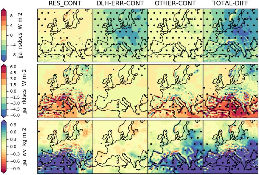
S. O. Tucker et al.

Fig. 2  Left DJF seasonal mean observed, left-centre t RCM-PPE       used as observations), middle row: surface air temperature, bottom
biases, right-centre GCM-PPE biases, right differences between RCM   row: precipitation
and GCM. Top row: sea level pressure (ERA-INTERIM reanalysis is

   RCM-PPE and GCM-PPE ensemble mean biases have                     S2). It is also worth noting that for mountainous regions
similar spatial patterns and magnitudes. In particular both          such as the Alps and Norway, Cornes et al. (2018) report
ensembles have a cold bias that reaches 8 K over Scandina-           a discrepancy between the E-OBS values and those from
via. The magnitude of the bias over Scandinavia is however           NMSs, with E-OBS warmer on average by more than 5 °C
slightly reduced in RCM-PPE and is largely removed in                across the high Alps. This discrepancy is likely the result of
ERAI-RCM-STD except over Norway (supplementary figure                there being more high‐elevation stations available for the

13
Evaluation of a new 12 km regional perturbed parameter ensemble over Europe

MeteoSwiss interpolation. The ERAI-RCM-STD results                         between the two ensembles the RCM-PPE is around 0.5 K
suggest that the Scandinavian cold bias is largely inherited               cooler than the GCM-PPE, and like winter the RCM-PPE
from the driving GCM. Reasons for the cold bias in GCM-                    is ~ 0.3 mm/day wetter. The temperature difference means
PPE are discussed in the UKCP report (Murphy et al. 2018),                 that the South East European warm bias is smaller in RCM-
and contributing factors include a strong aerosol forcing.                 PPE, whilst the cold bias in the North East of the domain
Additionally, McSweeney et al. (2021) find that GCM-PPE                    is larger.
members with the largest Scandinavian cold biases also                         Warm dry summer biases in South East Europe are also
have the weakest circulation over the Atlantic. Consistent                 found in EURO-CORDEX evaluation (reanalysis driven)
with this, McDonald et al. (prep) find that the members with               simulations (Kotlarski et al. 2014), and are believed to be
fewer storms over the UK are drier and colder over Europe.                 related to local soil moisture feedbacks in a soil moisture-
Thus, variations in mean circulation seem to play a role                   controlled evaporative regime. Specifically, where evapora-
in explaining variations in the cold bias across members.                  tion from the surface is limited by available soil moisture,
Both the GCM-PPE and RCM-PPE ensembles have a wet                          the amount of energy used for latent heat flux decreases
bias over almost the entire domain, with the bias slightly                 and sensible heat flux increases, leading to an increase of
(~ 0.3 mm/day) worse in RCM-PPE.                                           air temperature (e.g., Seneviratne et al. 2010). Supporting
    In addition to ensemble mean maps, in supplementary                    this, Knist et al. (2017) investigate land atmosphere cou-
figure (S4) we show boxplots for the different PRUDENCE                    pling strength in the same set of simulations and find it tends
analysis regions to see the spread among members. These                    to be too strong in this region. We note as an aside from
regions are intended to provide homogeneous climatic con-                  boxplots of the Mediterranean (MD) and East Europe (EA)
ditions and have been used to allow easy comparison with                   region (Supplementary figure S7) that warm and dry and
results from EURO-CORDEX studies (such as Kotlarski                        wet biases are not present consistently in the GCM driven
et al. 2014). For reference, a EURO-CORDEX box is also                     EURO-CORDEX simulations, suggesting that errors other
included for the 32 0.11° RCM EURO-CORDEX simula-                          than too strong land atmosphere coupling may be compen-
tions we were able to plot using ESMValTool (Righi 2020)                   sating. Support for a soil moisture feedback explanation in
(a full list of included simulations is included in the figure             our ensembles is provided by supplementary figure S8, the
caption). For Scandinavia, 11 out of 12 UKCP18 RCM-                        top panel shows a scatter plot of South East Europe sur-
PPE members have a cold bias with strong correlations                      face air temperature and evaporation, that shows negative
between RCM and driving GCM-PPE members. The plot                          correlations between these variables in both RCM-PPE and
shows that the cold bias is not systematic in the EURO-                    GCM-PPE. Further the middle panel show that evaporation
CORDEX ensemble, and furthermore simulations using the                     is correlated with 850 hPa specific humidity, so reduced
MOHC-HadREM3-GA7-05 RCM (same as our RCM-STD                               evaporation reduces the amount of moisture available for
but driven by different GCMs) span a significant part of the               precipitation (and thus the soil stays dry). Supplementary
spread in EURO-CORDEX temperatures. This provides fur-                     figure S8 bottom panel shows that all GCM-PPE members
ther evidence that the cold bias is inherited from the driving             are warmer and drier than observations, nine out of twelve
UKCP18 GCM-PPE. It is also of note that the same member                    RCM-PPE members are warmer than the observed, and
is the warmest in winter for all regions in both RCM-PPE                   nine out of twelve RCM-PPE members are wetter than the
and GCM-PPE.                                                               observed. Additionally we note from the top panel of Fig. 3
    Scatter plots of land only surface air temperature and pre-            that PMSL biases are small (less than 3 hPa) suggesting
cipitation (supplementary figure S7 top) show that warmer                  that large scale circulation differences are unlikely to be the
members tend to be wetter. Both land only surface air tem-                 cause of the large temperature biases, although we do note
perature (supplementary figure S7 middle) and precipita-                   that in both ensembles there appears to be a northward shift
tion (supplementary figure S7 bottom) correlate well with                  in the Azores high that may cause more blocking conditions
domain averaged 850 hPa specific humidity. We observe that                 over central Europe.
warmer members tend to be wetter because specific humid-                       The large-scale circulation consistency between the driv-
ity is higher and therefore more water is available for precip-            ing global and regional models is further assessed at the
itation. We also note that there is a high level of consistency            daily time scale. For each day the spatial correlation of sea
between RCM-PPE and GCM-PPE in terms of correlation                        level pressure between the RCM and GCM has been calcu-
between RCM members and their driving GCM members                          lated, supplementary table S1 shows the 25th, 50th and 75th
(i.e. the warmest and wettest GCM members being also the                   percentile of the correlations for each member. In winter the
warmest and wettest RCM members).                                          median correlation is above 0.97 for all members, and in
    Figure 3 shows similar results for summer, where both                  summer above 0.90. The correlations found here are gener-
ensembles have a cold bias over Scandinavia, but a warm                    ally higher than those found in EURO-CORDEX simulations
and dry bias over South East Europe. In terms of differences               (Vautard et al. 2020), which may be due to each RCM-PPE

                                                                                                                               13
S. O. Tucker et al.

Fig. 3  As Fig. 2, but for JJA

and GCM-PPE member having the same atmosphere and                  boundary conditions and/or aerosol differences. ERAI-
land surface configuration. These results provide further          RCM-STD temperature is a clear improvement over Scan-
evidence that precipitation and temperature differences are        dinavia, but over SE Europe the warm bias is enhanced.
not due to large scale circulation differences.                       In summary, there is generally good large scale consist-
   Supplementary figure S3 shows that ERAI-RCM-STD                 ency between RCM-PPE and GCM-PPE in both seasons,
is warmer than RCM-STD over land despite having cooler             both in terms of correlations between members (domain
SSTs. This is an interesting result that requires further inves-   average correlations above 0.9 for all variables and sea-
tigation, but which must be due to either different lateral        sons) and spatial patterns of the ensemble mean. In winter

13
Evaluation of a new 12 km regional perturbed parameter ensemble over Europe
this means that RCM-PPE inherits a large cold bias over simulations to try and unpick what configuration differences
Scandinavia. Despite the generally good large scale con- cause the differences between the RCM and GCM.
sistency, RCM-PPE JJA ensemble mean is cooler by 0.5 K
on average, with all RCM members being cooler than their 3.2.1 Clouds and radiation
driving GCM. Additionally, in both seasons RCM-PPE is
wetter than GCM-PPE in both seasons by ~ 0.3 mm/day. We Figure 5 shows DJF cloud cover, and shortwave and long-
investigate these differences in the next section. wave cloud radiative forcing at the top of the atmosphere.
Both ensembles have more cloud cover than observed
3.2 Causes of differences in temperature (domain average bias 13% in RCM-PPE and 10% in GCM-
and precipitation PPE), with the bias being greater over land than sea. Despite
the positive cloud cover bias, both ensembles have a positive
Surface temperature is ultimately determined by the net shortwave cloud forcing bias, and negative longwave cloud
effect of many drivers. Such drivers can include remote forcing bias. This suggests that other errors in the represen-
influences on atmospheric heat and moisture convergence tation of clouds (possibly clouds being too thin) are offset-
into the region, plus local effects such as clouds, precipita- ting the cloud cover biases.
tion, aerosols, boundary layer mixing, snow cover and soil Figure 6 is for JJA. Cloud cover is increased in RCM-PPE
properties including soil moisture content. These drivers can compared to GCM-PPE (domain average absolute difference
both respond to and modify the state variables, and impact of 6.5%). As both ensembles under simulate cloud cover for
surface air temperature via the surface energy budget (radia- the majority of the domain, this represents an improvement
tive fluxes, conductance into the deep soil, sensible heat flux in RCM-PPE. Unlike in DJF, radiative forcing biases seem
and latent heat flux). to simply follow the cloud cover differences, this means that
To illustrate some of the terms in the surface energy cloud forcing biases are reduced in RCM-PPE over the parts
budget, Fig. 4 shows JJA downward surface radiative flux of the domain where cloud cover is under-estimated.
(shortwave plus longwave), surface upward radiative flux, Supplementary figures S8 (DJF) and S9 (JJA) show that
latent heat flux and sensible heat flux. In GCM-PPE there is cloud cover bias is reduced in ERAI-RCM-STD compared
too much downward (i.e. incoming) surface radiation over to RCM-STD, suggesting that the bias is partially inher-
the UK and central Europe. In terms of differences between ited from GCM-PPE. The magnitudes of the differences are
RCM-PPE and GCM-PPE, RCM-PPE has less downward generally small, but it is of note that in the North East of
(and net) radiation, which may be due to differences in cloud the domain there is a large (~ 20 W m−2) difference in JJA
cover. The latent heat flux is higher over parts of the Medi- shortwave cloud forcing, which are likely contributing to the
terranean Sea, and South East Europe. For the latter region warmer surface temperatures in ERAI-RCM-STD.
this is consistent with the idea that soil moisture feedbacks We also note that for DJF, biases in net downward surface
are enhancing the temperature differences between the two radiation are negative for shortwave and positive for long-
ensembles. Both upward radiation and sensible heat flux is wave (supplementary figure S10). This is the opposite sign
lower than in GCM-PPE, consistent with the temperature to the cloud radiative forcing biases, meaning that the largest
being lower in the RCM-PPE. radiative forcing biases are coming from clear-sky rather
Full analysis of the temperature differences between than cloud processes. In contrast, JJA net surface radiation
ensembles would involve analysing all the various drivers biases (supplementary figure S11) are largely similar to
and their interactions. The focus of this subsection however, cloud radiative forcing biases.
is the analysis of clouds and their radiative effects in order to
isolate their contribution to the summertime temperature dif- 3.2.2 Sensitivity simulations
ferences between RCM-PPE and GCM-PPE. This is partly
motivated by the differences in downward (shortwave plus In terms of what is causing the cloud and radiation differ-
longwave) radiation above, and also the fact that cloud cover ences between the RCM and GCM, model development
is known to be influenced by resolution. We find that cloud tests show a cloud sensitivity to resolution in GA7, with
cover is considerably higher in RCM-PPE than in GCM- higher resolutions having an increased summertime cloud
PPE. In general, increased cloud cover causes a decrease in cover of ~ 5% around the UK. However, the increased
downward surface shortwave radiation and an increase in cloud cover goes with a reduced optical depth and so the
downward longwave radiation. However, the cloud radiative radiative variation with resolution is smaller. We there-
effect is also dependent on a number of factors including the fore might expect to see cloud differences with resolution.
height of the cloud, and the cloud thickness. In Sect. 3.2.1, In terms of other configuration differences, we speculate
we analyse how cloud cover and surface radiation diagnos- that the most notable is the treatment of aerosols. In Bel-
tics compare to observations. In Sect. 3.2.2, we use the extra louin and Thornhill (2018), it is found that the simulation
13S. O. Tucker et al. Fig. 4 JJA. Top row surface downward radiation (longwave + short- upward radiation. Bottom row left is the latent heat flux in GCM- wave). Top row left is the observed estimate from CERES, top row PPE, bottom row second panel is the difference in latent heat flux second from left is the bias in RCM-PPE, third from left the bias in between RCM-PPE and GCM-PPE. Bottom row third from left is the GCM-PPE and on the right the difference between RCM-PPE and sensible heat flux in GCM-PPE, and bottom row right is the differ- GCM-PPE Second row is the same as the top row, but for surface ence in sensible heat flux between RCM-PPE and GCM-PPE 13
Evaluation of a new 12 km regional perturbed parameter ensemble over Europe

Fig. 5  First left DJF seasonal mean observed, third from right RCM-PPE biases, second from right GCM-PPE biases, right differences between
RCM and GCM. Top row: cloud cover, middle row: shortwave cloud radiative effect, bottom row: downward longwave surface radiation

using EasyAerosol has increased liquid cloud cover, and                    replicate in the RCM the effects of explicit aerosol model-
consequently reduced downward shortwave, and increased                     ling included in the driving GCM. In the rest of this sub-
downward longwave radiation. In addition, there is also the                section we use the RCM-LOWRES and RCM-LOWRES-
DLH-error in the prescribing of EasyAerosol shortwave                      DLHFIX simulations to determine which differences are
extinction and absorption properties. Any differences due                  due to resolution, which are due to the error, and which are
to the use of EasyAerosol, and in particular the day light                 due to other differences. Specifically, we look at:
hours error is undesirable as the scheme is intended to

                                                                                                                               13
S. O. Tucker et al.
Fig. 6 As Fig. 5, but for JJA
• RCM-STD-RCM-LOWRES to see what differences are error, believed to be dominated by the different treat-
due to resolution (RES-CONT) ment of aerosols (OTHER-CONT)
• RCM-LOWRES-RCM-LOWRES-DLHFIX to see what • RCM-STD-GCM-STD showing the total difference
differences are due to the daylight hours error (DLH- between the two simulations (TOTAL-DIFF)
ERR-CONT)
• RCM-LOWRES-DLHFIX-GCM-STD to see what dif- We speculate that the differences between RCM-
ferences are not due to either resolution or the DLH LOWRES-DLHFIX and GCM-STD (OTHER-CONT) are
13Evaluation of a new 12 km regional perturbed parameter ensemble over Europe
dominated by the treatment of aerosols, however other dif- 3. The RCM has a lower (~ 40 km) upper lid.
ferences between the two runs are described in Sect. 2.2 and 4. A couple of schemes are only available in global mod-
summarised as. els, namely a stochastic physics package (Sanchez et al.
2016), and the TRIP (Total Runoff Integrating Pathways
1. The RCM-LOWRES-DLHFIX is an atmosphere only model: Oki and Sud 1998) river routing scheme.
model with prescribed SST and sea ice from GCM-STD,
whilst GCM-STD includes coupled ocean and sea ice We show figures for JJA with corresponding figures
models. for DJF in supplementary material (figures S12, S13 and
2. The RCM-LOWRES-DLHFIX is a limited area model S14). Figures 7, 8 and 9 the left hand column shows
covering the EURO-CORDEX domain, with informa- RES-CONT, second from left column shows DLH-ERR-
tion passed from GCM-STD at the lateral boundaries. CONT, third from left column shows OTHER-CONT and
Additionally, the land sea mask has been produced from the right hand side shows TOTAL-DIFF. Due to only hav-
a different source and so will differ from the GCM mask. ing 10 years of data for RCM-LOWRES, a paired t-test
Most notably lakes Onega and Ladoga stand out in the has been performed to determine whether differences are
plots.
Fig. 7 JJA. Left column shows differences between RCM-STD and row: surface air temperature, second row: precipitation, third row:
RCM-LOWRES (RES-CONT), second from left column differences downward shortwave surface radiation, bottom: downward longwave
between RCM-LOWRES and RCM-LOWRES-DLHFIX (DLH- surface radiation. All plots are seasonal means for the 10 year period
ERR-CONT), third from left differences between GCM-STD and that RCM-LOWRES was run for. Dots indicate areas where differ-
RCM-LOWRES-DLHFIX (OTHER-CONT), and right column shows ences are statistically significant at the 5% level. Note that the long-
differences between RCM-STD an GCM-STD (TOTAL-DIFF). Top wave and shortwave plots have different scales
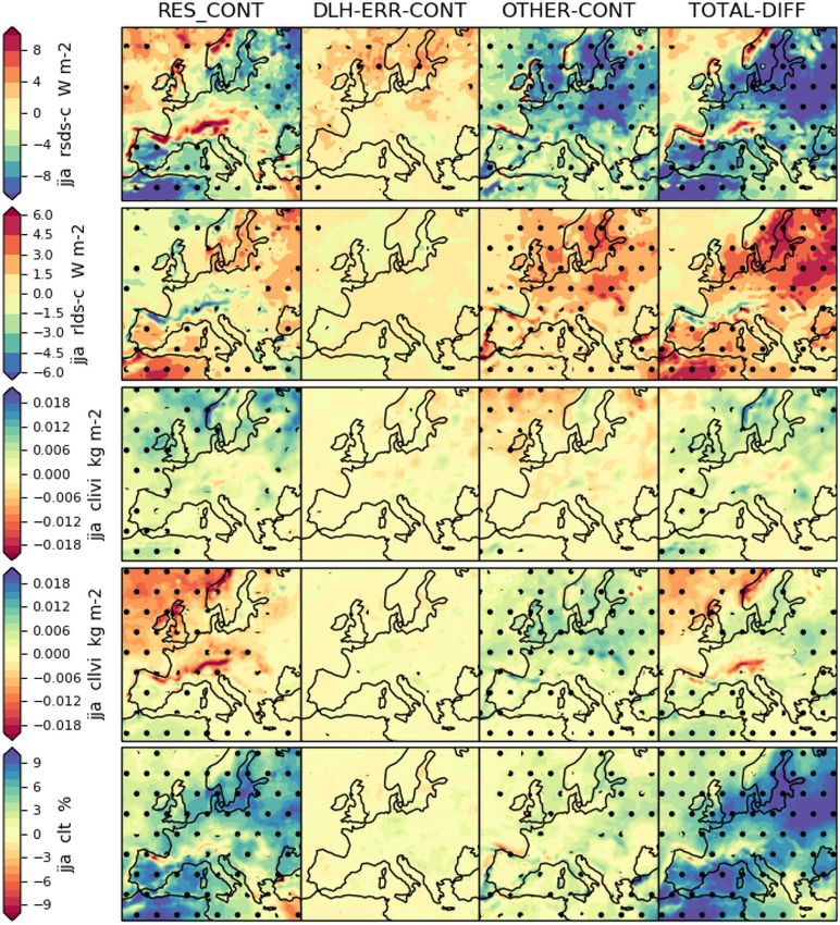
13S. O. Tucker et al. Fig. 8 JJA clear sky differences. Left column shows differences surface radiation, second row clear sky downward longwave surface between RCM-STD and RCM-LOWRES (RES-CONT), second radiation, bottom: total atmospheric water vapour. All plots are sea- from left column differences between RCM-LOWRES and RCM- sonal means for the ten year period that RCM-LOWRES was run for. LOWRES-DLHFIX (DLH-ERR-CONT), third from left differ- Dots indicate areas where differences are statistically significant at ences between GCM-STD and RCM-LOWRES-DLHFIX (OTHER- the 5% level. Note that the longwave and shortwave plots have differ- CONT), and right column shows differences between RCM-STD an ent scales GCM-STD (TOTAL-DIFF). Top row: clear sky downward shortwave significant: the areas where the differences are statistically resolution due to a stronger hydrological cycle as well as significant at the 5% level are marked with dots. local effects in the vicinity of mountains/coast due the better The top row of Fig. 7 shows temperature differences, representation of topography at high resolution. Our results where RES-CONT shows a clear orography footprint with bear this out, with resolution causing an increase in pre- the Pyrenees, Alps, Carpathian, Scandinavian and Scottish cipitation over the Atlantic, and local effects in the vicinity mountain ranges clearly identifiable. Correspondingly high of mountains. Reassuringly the DLH-error is having little elevation areas have increased downward shortwave (third impact on precipitation differences. Other differences are row), and decreased downward longwave (bottom row). In also contributing to increased precipitation over large areas addition to orographic features, higher resolution is causing of central and eastern Europe. a cooling over Finland. As expected, the day light hours TOTAL-DIFF radiation differences are of opposite signs error is causing a reduction in downward shortwave radiation for longwave and shortwave, however the negative short- and no impact on longwave, as a consequence of this DLH- wave differences are of a larger magnitude than longwave ERR-CONT is cooler over large areas of central and East- differences leading to a net negative downward radiation dif- ern Europe by up to 0.4 K. It should be noted that the day ference consistent with RCM-STD being cooler. The same light hours error is typically contributing less than a third reverse pattern between long and short wave differences can of the total surface air temperature difference, and OTHER- be seen in RES-CONT and OTHER-CONT, with both con- CONT is the largest contributor to the total summertime tributing to the total difference. cold difference. In the next two figures we further split the radiation dif- Precipitation differences are on the second row. Based ferences in to cloud and clear sky differences. Bellouin and on previous experience (e.g. Jones et al. 1995, 1997; Prein Thornhill (2018) attribute radiative imbalances resulting et al. 2016) we expect to see more precipitation at higher from the use of EasyAerosol as due to the interactions of 13
Evaluation of a new 12 km regional perturbed parameter ensemble over Europe

Fig. 9  JJA cloud differences. Left column shows differences between       to clouds (rsds—rsdscs), second row: downward longtwave surface
RCM-STD and RCM-LOWRES (RES-CONT), second from left                        radiation due to clouds (rlds—rldscs), third row: total cloud ice con-
column differences between RCM-LOWRES and RCM-LOWRES-                      tent, fourth row: total cloud water content, bottom: cloud area frac-
DLHFIX (DLH-ERR-CONT), third from left differences between                 tion. All plots are seasonal means for the 10 year period that RCM-
GCM-STD and RCM-LOWRES-DLHFIX (OTHER-CONT), and                            LOWRES was run for. Dots indicate areas where differences are
right column shows differences between RCM-STD an GCM-STD                  statistically significant at the 5% level. Note that the longwave and
(TOTAL-DIFF). Top row: downward shortwave surface radiation due            shortwave plots have different scales

aerosols and clouds, consequently this partitioning allows us              DLH-ERR-CONT (ignoring locations where there is a land
to check whether our findings are consistent. Additionally,                sea mask difference). Once the error is removed the remain-
looking at cloud properties allows us to explore the cloud                 ing clear sky differences largely correspond to where there
sensitivity to resolution observed in GA7 development.                     are differences in atmospheric water vapour (bottom row).
   Figure 8 top row shows differences in downward clear-                   RES-CONT is showing orographic features as well as a large
sky surface radiation. It can be seen that around 80% of                   positive difference in the South West of the domain. A possi-
the negative clear sky radiation differences are due to                    ble explanation for the increased evaporation in RES-CONT

                                                                                                                                     13
S. O. Tucker et al.
could be stronger surface winds, possibly due to the RCM contributions being of opposite sign. Additionally, over the
generating more frequent or more intense storms in an Atlantic, there are differences in cloud properties between
area that includes two cyclogenesis regions (Trigo 1999). the RCM and GCM, with increases in ice cloud amount
OTHER-CONT shows positive differences in the South East and cloud area, but decreases in liquid cloud, which act
of the domain. to compensate for each other in terms of radiative effects.
Figure 9 shows differences in downward surface cloud Similar plots for winter are shown in supplementary
radiative effects (total downward short/long wave radia- material (figures S13, S14 and S15. We see that Easy-
tion − clear sky downward short/long wave radiation). Aerosol introduces a warm difference in winter (around
Typically, where shortwave differences are negative/posi- 0.4–0.8 K) over France and Germany that is not detected
tive, longwave differences are positive/negative, with the as statistically significant in the total difference between
magnitude of the longwave differences roughly half that of the RCM and GCM, presumably due to increased vari-
the shortwave. ability in the RCM. Resolution generally causes a similar
RES-CONT has an increase in cloud cover over practi- change in cloud properties in winter as it did in summer,
cally the entire domain (bottom row), with an absolute dif- although some parts of Southern Europe, such as Northern
ference exceeding 5% over the North East of the domain Spain, Italy, and the Balkans are an exception: in these
(everything North East of a line drawn from Oslo to Istan- regions resolution causes a reduction in cloud, and thus a
bul), the West Mediterranean and North Africa. We might reduction in downwards longwave and increase in down-
therefore expect a decrease in downward shortwave radia- wards shortwave.
tion, and an increase in longwave radiation, and indeed this In conclusion, the summertime temperature difference
is largely the case, for example over Spain there is a negative between the RCM and GCM comes predominantly from
shortwave difference of over 6 W m−2, and positive long- other differences, believed to be EasyAerosol. Other differ-
wave difference of around 3 W m−2. However over other ences also introduce a warm difference in winter over France
parts of the domain it is more complicated. For example, and Germany. Our findings are consistent with those of in
over the Atlantic in the North West of the domain, despite a Bellouin and Thornhill (2018), who found that the simu-
small increase in cloud cover, there is a positive shortwave lation using EasyAerosol increased liquid cloud cover and
difference (of ~ 4 W m−2), and a negative longwave differ- thickness, and consequently reduced downward shortwave,
ence (of 0–2 W m−2). In this region we see a widespread and increased downward longwave radiation. These differ-
reduction in liquid cloud amount, but an increase in cloud ences are further traced to the prescribing of monthly mean
ice. Since liquid clouds tend to be lower and more reflec- cloud droplet number concentrations. As the intention of
tive, this will act to decrease the downward longwave and EasyAerosol was to replicate the effects of the aerosol mod-
increase the downward shortwave. The main exception to elling in the GCM, these differences are undesirable.
increased cloud cover, is mountainous regions with the Alps, It is of note that the RCM’s summertime cold, and win-
Pyrenees, and highland areas of Scotland and Norway stand- ter warm difference over Scandinavia is a genuine conse-
ing out. In these regions a reduction in cloud thickness is quence of resolution. As is increased rainfall in both seasons
causing a reduction in the cloud radiative effect. over the Atlantic, and over Spain in JJA. These differences
OTHER-CONT sees negative shortwave differences over may be related to different cloud properties in the RCM,
the majority of the domain, with a strong spatial correlation that include a change in vertical distribution, an increase in
between these and increases in liquid cloud amount. Easy- cloud cover, but reduced cloud thickness. These differences
Aerosol does not directly interact with ice clouds, and for may represent an improvement, but to establish this and to
most of the domain we do not see any ice cloud differences, gain further understanding of cloud sensitivity to resolution
however in the Northern part over the Atlantic there is a requires further investigation, which is beyond the scope of
small decrease. To further illustrate the changes in the verti- the current study.
cal distributions of clouds, vertical profiles are shown in sup-
plementary figure S15, OTHER-CONT shows an increased
cloud amount at low levels (peak difference around 2 km), 3.3 Evaluation of daily distributions
whilst RES_CONT shows a reduction in low level clouds,
but increase in high clouds. In this subsection, we analyse daily precipitation
Overall, in summer there is an increased cloud radiative (Sect. 3.3.1) and temperature (Sect. 3.3.2) distributions, two
effect in the RCM, with negative shortwave differences variables that are important from an impacts perspective.
being larger than the positive longwave differences. The As before we restrict ourselves to analysing data on the low
exception being over the North West of the domain over resolution grid, to allow a fair comparison between RCM-
the Atlantic. The differences over the Atlantic largely can- PPE and GCM-PPE. We note however that RCM-PPE may
cel each other out, with RES-CONT and OTHER_CONT have additional skill at smaller spatial scales.
13Evaluation of a new 12 km regional perturbed parameter ensemble over Europe
3.3.1 Precipitation regions in which it typically rains on fewer than 5% of
days, and the majority of the total rainfall falls on days
Figure 10 shows the percentage of seasonal mean precipi- where the rainfall exceeds the 99th percentile. Due to
tation that falls on days that have precipitation above the the large spatial variation in this statistic, relative rather
99th percentile of daily precipitation for that season (r99). than absolute error has been used to compare the different
This statistic has been chosen as we already know that datasets.
RCM-PPE is wetter on average, and instead here we want a In winter both ensembles underestimate the proportion
measure of the shape of the rainfall distribution. Reassur- of rainfall falling as extremes, over the majority of the
ingly there are typically no obvious changes in observed domain. The performance of RCM-PPE and GCM-PPE is
values along the boundaries where the source data has remarkably similar. In summer both ensembles have too
been switched. An exception may be the Russian border, much precipitation falling as extremes over the majority
that stands out in winter difference plots. This suggests of the domain, but the magnitude of the error is reduced in
that a lack of observations over Russia might be leading RCM-PPE (median absolute error reduced from 2.4 to 0.4,
to an underestimate of the contribution of extremes to the and relative error from 17.7 to 3.3%). RCM-PPE consist-
total rainfall. The observed spatial distribution is very ently has a lower contribution from extreme events than
non uniform, particularly in summer. The median sum- GCM-PPE over the whole domain, and this is largely an
mer value is 13%, but there are Southern Mediterranean improvement except over Southern Mediterranean regions.
Fig. 10 Left: the observed percentage of seasonal mean precipita- GCM-PPE. Top row DJF, bottom row JJA. In the labels, ‘mean’ refers
tion that falls on days that have precipitation above the 99th percen- to the spatial average value, ‘median’ is the spatial median of the field
tile of daily precipitation for that season (R99). Third from right: being shown, and ‘corr’ is the spatial correlation of the datasets being
relative RCM-PPE biases of R99, second from right: relative GCM- differenced
PPE biases of R99, right: relative differences between RCM-PPE and
13S. O. Tucker et al.
In order to gain a more in depth understanding of the high intensity events. Specifically, GCM-PPE has too many
differences in rainfall distributions, supplementary material days with less than 3 mm of rainfall.
(figures S16–S26) shows the fractional contribution of dif- To summarise, in winter both ensembles underestimate
ferent rainfall intensities to the total rainfall amount, for each dry day frequency by 30–50% depending on the region but
region that we have NMS observations for. As in Berthou do a generally good job at reproducing the observed inten-
et al. (2019), a logarithmic axis has been used on the inten- sity distribution. There is little difference in RCM-PPE and
sity (x) axis, with the graph constructed from exponentially GCM-PPE performance except for extreme intensities,
sized bins, so the total rainfall is proportional to the area where RCM-PPE performs better. Skill is generally lower in
under the curve as visualised. The following statistics are summer than winter, with both ensembles having too much
also reported: rainfall coming from low intensity days, however downscal-
ing leads to an improvement in the intensity distribution. We
r99, the percentage of total rainfall falling above the 99th have used r99 as a measure of the shape of the precipitation
percentile distribution and have found that RCM-PPE has higher val-
S, the common area of the model and observed distribu- ues in five out of six regions in winter, but lower values in
tions as defined in Perkins et al. (2007), (expressed here the summer. This is an improvement in 5 out of six regions
as a percentage) in winter, and 3 regions in summer. To conclude, we find
dav = 100(SRCM − SGCM)/SGCM, the distribution added that downscaling generally adds value, but not everywhere,
value as used by Soares and Cardoso (2018) to quantify and for summertime the dry day underestimation is actually
added value in downscaling worse in RCM-PPE.
dry_freq, the percentage of days with less than 0.1 mm
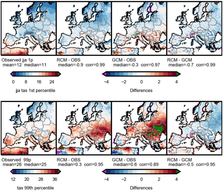
of rain. 3.3.2 Temperature
The fractional contribution plots reveal errors in the Figure 11 shows the ensemble mean of the 1st and 99th
distribution of rainfall intensity, whilst dry day frequency percentile of DJF daily temperature differences. In both
allows us to examine errors in rainfall occurrence. In win- ensembles the 1st percentile cold bias is generally larger
ter the dry day frequency is underestimated in both RCM- than the mean bias (Fig. 2), which in turn is larger than the
PPE and GCM-PPE by between a third and a half depend- cold bias in the 99th percentile. In other words, in addition
ing on region. In Scandinavia the under-simulation of dry to being too cold on average, the spread in the daily tempera-
days leads to a wet bias in the models, despite a very good ture distributions is too large. The first percentile of RCM-
distribution (SRCM = SGCM = 96%) of rainfall intensities. In PPE is warmer than GCM-PPE by 0.4 K on average, with
general, up until around the 99th percentile, the RCM-PPE some locations exceeding 3 K. This means the RCM-PPE
winter distributions for all regions are similar to that of has reduced the cold day bias present in the GCM-PPE, and
GCM-PPE, just slightly shifted towards higher intensities. furthermore RCM-PPE is showing an improvement in cold
However high intensities contribute more to the RCM’s total day extremes that goes beyond a simple shift of the entire
rainfall, resulting in the RCM having higher values of r99 daily temperature distribution.
in five out of six regions. These higher values of r99 are an Figure 12 shows the equivalent plot for JJA. The 99th
improvement for Great Britain, Scandinavia, France, and the percentile biases show a similar spatial pattern to the mean
Carpathians, but not for Iberia. biases, namely that both ensembles are too warm in South
In summer the under-simulation of dry days is reduced to East Europe, but too cool over Scandinavia. However, the
less than 20% for mainland European regions (Spain, France, 99th percentile warm bias is of greater magnitude and
the Alps and the Carpathians). For all regions however the extends further into central Europe than the mean bias, a
dry day frequency in RCM-PPE is worse than in GCM-PPE. finding consistent with our suggestion of soil moisture feed-
Just like in winter, the intensity distribution for Scandinavia backs. Just like the seasonal mean temperature, RCM-PPE
has excellent skill in both RCM-PPE (S = 97) and GCM-PPE is cooler than GCM-PPE everywhere which represents a
(S = 99), but both ensembles have a wet bias due to rain- bias reduction in the 99th percentile for South and central
ing too frequently. However, in all other regions the skill is Europe. Additionally, the spatial correlation with observa-
lower in summer than in winter, with too much rainfall being tions is higher in RCM-PPE (0.95) than in GCM-PPE (0.89).
contributed from low intensities (less than ~ 3 mm), and not Downscaling appears to be improving the distribution of
enough from moderate intensities (around 10 mm). This is daily temperature in winter, and hot extremes in summer.
true in both ensembles, but to a lesser extent in RCM-PPE We know from Sect. 3.2.2 that there are some differences
as reflected in positive dav scores. The positive summer r99 in mean temperature between the RCM and GCM that are
biases over mainland Europe appear due to differences in the not directly due to resolution. Such effects are also likely
bulk of the distribution, rather than in the contribution from to influence the tail of the distribution, however additional
13You can also read