High-resolution induced polarization imaging of biogeochemical carbon turnover hotspots in a peatland
←
→
Page content transcription
If your browser does not render page correctly, please read the page content below
Biogeosciences, 18, 4039–4058, 2021
https://doi.org/10.5194/bg-18-4039-2021
© Author(s) 2021. This work is distributed under
the Creative Commons Attribution 4.0 License.

High-resolution induced polarization imaging of biogeochemical
carbon turnover hotspots in a peatland
Timea Katona1 , Benjamin Silas Gilfedder2,4 , Sven Frei2 , Matthias Bücker3 , and Adrian Flores-Orozco1
1 Research   Division Geophysics, Department of Geodesy and Geoinformation, TU-Wien, Vienna, Austria
2 Department    of Hydrology, Bayreuth Center of Ecology and Environmental Research (BAYCEER),
University of Bayreuth, Bayreuth, Germany
3 Institute for Geophysics and Extraterrestrial Physics, TU Braunschweig, Braunschweig, Germany
4 Limnological Station, Bayreuth Center of Ecology and Environmental Research (BAYCEER),

University of Bayreuth, Bayreuth, Germany

Correspondence: Timea Katona (timea.katona@tuwien.ac.at)

Received: 23 November 2020 – Discussion started: 6 January 2021
Revised: 22 May 2021 – Accepted: 29 May 2021 – Published: 6 July 2021

Abstract. Biogeochemical hotspots are defined as areas             1   Introduction
where biogeochemical processes occur with anomalously
high reaction rates relative to their surroundings. Due to their
importance in carbon and nutrient cycling, the characteriza-       In terrestrial and aquatic ecosystems, patches or areas that
tion of hotspots is critical for predicting carbon budgets ac-     show disproportionally high biogeochemical reaction rates
curately in the context of climate change. However, biogeo-        relative to the surrounding matrix are referred to as biogeo-
chemical hotspots are difficult to identify in the environment,    chemical “hot spots” (McClain et al., 2003). Hotspots for
as methods for in situ measurements often directly affect the      turnover of redox-sensitive species (e.g., oxygen, nitrate, or
sensitive redox-chemical conditions. Here, we present imag-        dissolved organic carbon) are often generated at interfaces
ing results of a geophysical survey using the non-invasive         between oxic and anoxic environments, where the local pres-
induced polarization (IP) method to identify biogeochemi-          ence/absence of oxygen either favors or suppresses biogeo-
cal hotspots of carbon turnover in a minerotrophic wetland.        chemical reactions such as aerobic respiration, denitrifica-
To interpret the field-scale IP signatures, geochemical anal-      tion, or oxidation/reduction of iron (McClain et al., 2003).
yses were performed on freeze-core samples obtained in ar-         Biogeochemical hotspots are important for nutrient and car-
eas characterized by anomalously high and low IP responses.        bon cycling in various systems such as wetlands (Frei et al.,
Our results reveal large variations in the electrical response,    2010, 2012), lake sediments (Urban, 1994), the vadose zone
with the highest IP phase values (> 18 mrad) corresponding         (Hansen et al., 2014), hyporheic areas (Boano et al., 2014),
to high concentrations of phosphates (> 4000 µM), an indi-         or aquifers (Gu et al., 1998). Wetlands are distinct elements
cator of carbon turnover. Furthermore, we found a strong re-       in the landscape, which are often located where hydrological
lationship between the electrical properties resolved in IP im-    flow paths converge, such as at the bottoms of basin-shaped
ages and the dissolved organic carbon. Moreover, analysis of       catchments, local depressions, or around rivers and streams
the freeze core reveals negligible concentrations of iron sul-     (Cirmo and McDonell, 1997). Wetlands are attracting in-
fides. The extensive geochemical and geophysical data pre-         creasing interest because of their important contribution to
sented in our study demonstrate that IP images can track           water supply, water quality, nutrient cycling, and biodiver-
small-scale changes in the biogeochemical activity in peat         sity (Costanza et al., 1997, 2017). Understanding microbial-
and can be used to identify hotspots.                              moderated cycling of nutrients and carbon in wetlands is crit-
                                                                   ical, as these systems store a significant part of the global
                                                                   carbon through the accumulation of decomposed plant mate-
                                                                   rial (Kayranli et al., 2010). In wetlands, water table fluctua-

Published by Copernicus Publications on behalf of the European Geosciences Union.
4040                             T. Katona et al.: High-resolution induced polarization imaging of biogeochemical carbon

tions as well as plant roots determine the vertical and hor-       stance, Revil et al. (2017a) carried out IP measurements on a
izontal distributions of oxic and anoxic areas (Frei et al.,       large set of soil samples, for which they report a linear rela-
2012; Gutknecht et al., 2006). Small-scale subsurface flow         tionship between the magnitude of the polarization response
processes in wetlands, moderated by micro-topographical            and the cation exchange capacity (CEC) which is related to
structures (hollow and hummocks) (Diamond et al., 2020),           surface area and surface charge density.
can control the spatial presence of redox-sensitive solutes            Since the early 2010s, various studies have explored the
and formation of biogeochemical hotspots (Frei et al., 2010,       potential of IP measurement for the investigation of biogeo-
2012). Despite their relevance for the carbon and nutrient cy-     chemical processes in the emerging field of biogeophysics
cling, basic mechanisms controlling the formation and dis-         (Slater and Attekwana, 2013). Laboratory studies on sedi-
tribution of biogeochemical hotspots in space are not well         ment samples examined the correlation between the spectral-
understood.                                                        induced polarization (SIP) response and iron sulfide pre-
   Biogeochemically active areas traditionally have been           cipitation caused by iron-reducing bacteria (Williams et al.,
identified and localized through chemical analyses of point        2005; Ntarlagiannis et al., 2005, 2010; Slater et al., 2007;
samples from the subsurface and subsequent interpolation of        Personna et al., 2008; Zhang et al., 2010; Placencia Gomez
the data in space (Morse et al., 2014; Capps and Flecker,          et al., 2013; Abdel Aal et al., 2014). Further investigations
2013; Hartley and Schlesinger, 2000). However, such point-         in the laboratory have also revealed an increase in the polar-
based sampling methods may either miss hotspots due to the         ization response accompanying the accumulation of micro-
low spatial resolution of sampling (McClain et al., 2003) or       bial cells and biofilms (Davis et al., 2006; Abdel Aal et al.,
disturb the redox-sensitive conditions in the subsurface by        2010a, b; Albrecht et al., 2011; Revil et al., 2012; Zhang et
bringing oxygen into anoxic areas during sampling. Non-            al., 2013; Mellage et al., 2018; Rosier et al., 2019; Kessouri
invasive methods, such as geophysical techniques, have the         et al., 2019).
potential to study subsurface biogeochemical activity in situ          Motivated by these observations, the IP method has also
without interfering with the subsurface environment (e.g.,         been used to characterize biogeochemical degradation of
Williams et al., 2005, 2009; Atekwana and Slater, 2009; Flo-       contaminants at the field scale (Williams et al., 2009; Flores
res Orozco et al., 2015, 2019, 2020). Geophysical methods          Orozco et al., 2011, 2012b, 2013, 2015; Maurya et al., 2017).
permit us to map large areas in 3D and still resolve subsur-       Additionally, Wainwright et al. (2016) demonstrated the ap-
face physical properties with a high spatial resolution (Binley    plicability of the IP imaging method to identify naturally re-
et al., 2015).                                                     duced zones, i.e., hotspots, at the floodplain scale. These au-
   In particular, the induced polarization (IP) technique has      thors show that the accumulation of organic matter in areas
recently emerged as a useful tool to delineate biogeochem-         with indigenous iron-reducing bacteria results in naturally re-
ical processes in the subsurface (e.g., Kemna et al., 2012;        duced zones and the accumulation of iron sulfide minerals,
Kessouri et al., 2019; Flores Orozco et al., 2020). The IP         which are classical IP targets. In line with this argumenta-
method provides information about the electrical conductiv-        tion, Abdel Aal and Atekwana (2014) argued that the biogeo-
ity and the capacitive properties of the ground, which can be      chemical precipitation of iron sulfides controls the high elec-
expressed, respectively, in terms of the real and imaginary        trical conductivity and IP response observed in hydrocarbon-
components of the complex resistivity (Binley and Kemna,           impacted sites. Nonetheless, in a recent study, Flores Orozco
2005). The method is commonly used to explore metallic             et al. (2020) demonstrated the possibility of delineating bio-
ores because of the strong polarization response associated        geochemically active zones in a municipal solid waste land-
with metallic minerals (e.g., Marshall and Madden, 1959;           fill even in the absence of iron sulfides. Flores Orozco et
Seigel et al., 2007). Pelton et al. (1978) and Wong (1979)         al. (2020) argued that the high content of organic matter it-
proposed the first models linking the IP response to the size      self might explain both the high polarization response and
and content of metallic minerals. More recently, the role of       high rates of microbial activity, thus opening up the pos-
chemical and textural properties in the polarization of metal-     sibility of delineating biogeochemical hotspots that are not
lic minerals has been investigated in detail based on further      related to iron-reducing bacteria. This conclusion is consis-
developments of Wong’s model of a perfect conductor and            tent with previous studies performed in marsh and peat soils,
reaction currents (Bücker et al., 2018, 2019), while Revil et      areas with a high organic matter content and high micro-
al. (2012, 2015a, b, 2017b, c, 2018) have presented a new          bial turnover rates (Mansoor and Slater, 2007; McAnallen
mechanistic model that takes into account the intragrain po-       et al., 2018). Peat soils are characterized by a high surface
larization and Feng et al. (2020) have explained the polar-        charge and have been suggested to enhance the IP response
ization of perfectly conducting particles based on a Stern-        (Slater and Reeve, 2002). Mansoor and Slater (2007) con-
layer capacitance. The two latter groups of models do not in-      cluded that the IP method is a useful tool to map iron cy-
volve reaction currents. In porous media without a significant     cling and microbial activity in marsh soils. Garcia-Artigas
metallic content, the IP response can be related to the polar-     et al. (2020) demonstrated that bioclogging by bacteria in-
ization of the electrical double layer formed at the grain–fluid   creases the IP response accompanying wetland treatment.
interface (e.g., Revil and Florsch, 2010; Revil, 2012). For in-    Uhlemann et al. (2016) found differences in the electrical

Biogeosciences, 18, 4039–4058, 2021                                                  https://doi.org/10.5194/bg-18-4039-2021
T. Katona et al.: High-resolution induced polarization imaging of biogeochemical carbon                                        4041

resistivity of peat according to saturation, microbial activ-      riparian peatlands have developed around the major streams.
ity, and porewater conductivity; however, their study was          The plot-scale study site (Fig. 1c) is located in a riparian peat-
limited to direct-current resistivity and did not investigate      land draining into a nearby stream close to the catchment’s
variations in the IP response. In contrast to these observa-       outlet (Fig. 1b).
tions, laboratory studies have shown a low polarization re-           The groundwater level in this area annually varies within
sponse in samples with a high organic matter content, de-          the top 30 cm of the peat soil, and the local groundwater
spite its high CEC (Schwartz and Furman, 2014). Based on           flow has a S–SW orientation (Durejka et al., 2019) towards
field measurements, McAnallen et al. (2018) found that ac-         a nearby drainage ditch. Permanently high water saturation
tive peat is less polarizable due to variations in groundwa-       of the peat soil favors the development of anoxic biogeo-
ter chemistry imposed by sphagnum mosses, while degrad-            chemical processes close to the surface. Frei et al. (2012)
ing peat resulted in low resistivity values and a high polar-      suggested that hotspots in the study area are related to the
ization response. Based on measurements with the Fourier           stimulation of iron-reducing bacteria and accumulation of
transform infrared (FTIR) spectroscopy in water samples,           iron sulfides, which are generated by small-scale subsurface
the authors concluded that the carbon–oxygen (C=O) dou-            flow processes and the spatially non-uniform availability of
ble bond in degrading peat correlated with the polarization        electron acceptors and donors induced by the typical micro-
magnitude of the peat material. Based on laboratory inves-         topography of the peatland. Non-uniform availability of elec-
tigations, Ponziani et al. (2011) also concluded that decom-       tron acceptors and donors in combination with labile carbon
position of peat occurs predominantly by aerobic respiration,      stocks is the primary driver in generating biogeochemical
i.e., using molecular oxygen as the terminal electron accep-       hotspots in the peatland (Frei et al., 2012; Mishra and Riley,
tor to oxidize organic matter. Thus decomposition rates are        2015).
expected to be highest at the interface between the oxic and
anoxic zones.                                                      2.2   Experimental plot and geochemical measurements
   Based on these promising previous results, we hypothesize
that the IP method is a potentially useful tool for in situ in-    The experimental plot for the geophysical measurements
vestigation of biogeochemical processes and the mapping of         covers approximately 160 m2 (12.6 × 12.6 m, Fig. 1c) of the
biogeochemical hotspots. However, different responses ob-          riparian peatland. Sphagnum Sp. (peat moss) and Molinia
served in lab and field investigations do not offer a clear in-    caerulea (purple moor grass) dominate the vegetation, with
terpretation scheme of general validity. Additionally, it is not   the sphagnum and purple moor-grass abundance being higher
clear whether the IP method is only suited to characterizing       in the northern part of the plot (Fig. 2a and b). In the south-
biogeochemical hotspots associated with iron-reducing bac-         eastern region, where the sphagnum is less abundant, per-
teria, which favor the accumulation of iron sulfides. Hence,       manent surface runoff was observed (Fig. 2d). Peat thick-
in this study we present an extensive IP imaging data set col-     ness was measured with a 1 m resolution in the E–W direc-
lected at a peatland site to investigate the controls on the IP    tion and 0.5 m resolution in the N–S direction (along the IP
response in biogeochemically active areas. IP monitoring re-       profiles described below). To measure the thickness of the
sults are compared to geochemical data obtained from the           peat, a stainless-steel rod (0.5 cm in diameter) was pushed
analysis of freeze cores and porewater samples. Our main           into the ground until it reached the granitic bedrock (sim-
objectives are (i) to assess the applicability of the IP method    ilarly to Parry et al., 2014). The local groundwater level
to spatially delimit highly active biogeochemical areas in the     was measured in two piezometers and was found at ∼ 5–
peat soil and (ii) to investigate whether the local IP response    8 cm below the surface during the IP survey. Groundwater
is related to the accumulation of iron sulfides or high organic    samples were collected at three different locations (S1, S2,
matter turnover.                                                   and S3 indicated in Fig. 3) using a bailer. Porewater pro-
                                                                   files were taken at S1, S2, and S3 at 5 cm intervals to a
                                                                   maximum depth of 50 cm below ground surface (b.g.s.) us-
2     Material and methods                                         ing stainless-steel mini-piezometers. All water samples were
                                                                   filtered through 0.45 µm filters and analyzed for fluoride,
2.1    Study site                                                  chloride, nitrite, bromide, nitrate, phosphate, and sulfate us-
                                                                   ing an ion chromatograph (Compact IC plus 882, Metrohm
The study site is part of the Lehstenbach catchment located        GMBH). Dissolved organic carbon (DOC) was measured
in the Fichtelgebirge mountains (Fig. 1a), a low mountain          using a Shimadsu TOC analyzer via thermal combustion.
range in northeastern Bavaria (Germany) close to the border        Dissolved iron species (Fe2+ ) and total iron (Fetot ) con-
with the Czech Republic. Various soil types including Dys-         centrations were measured photometrically using the 1,10-
tric Cambisols, Haplic Podsols, and Histosols (i.e., peat soil)    phenanthroline method on porewater samples that had been
cover the catchment area of approximately 4.2 km2 , situated       stabilized with 1 % vol / vol 1 M HCl in the field (Tamura
on top of variscan granite bedrock (Strohmeier et al., 2013).      et al., 1974). Two freeze cores (see Fig. 2d) were extracted
The catchment is bowl shaped (Fig. 1b), and minerotrophic          at locations S1 and S2 (Fig. 3) by pushing an 80 cm long

https://doi.org/10.5194/bg-18-4039-2021                                                    Biogeosciences, 18, 4039–4058, 2021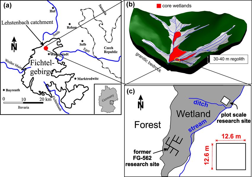
4042                              T. Katona et al.: High-resolution induced polarization imaging of biogeochemical carbon

Figure 1. (a) General overview of the experimental plot located in the Fichtel Mountains and (b) structure of the bowl-shaped Lehstenbach
catchment and (c) location of the experimental plot.

stainless-steel tube into the peat. After the tube was installed,      second pair of electrodes is used to measure the resulting
it was filled with a mixture of dry ice and ethanol. After             electrical potential (potential dipole). Modern devices can
around 20 min, the pipe with the frozen peat sample was ex-            measure tens of potential dipoles simultaneously for a given
tracted and stored on dry ice for transportation to the labo-          current dipole, permitting the collection of dense data sets
ratory at the University of Bayreuth. Both freeze cores were           within a reasonable measuring time. This provides an imag-
cut into 10 cm segments. Each segment was analyzed for re-             ing framework to gain information about lateral and verti-
active iron (1 M HCl extraction and measured for Fetot as de-          cal changes in the electrical properties of the subsurface. IP
scribed above) (Canfield, 1989), reduced sulfur species using          data can be collected in the frequency domain (FD), where
the total reduced inorganic sulfur (TRIS) method (Canfield et          an alternating current is injected into the ground where the
al., 1986) and carbon and nitrogen concentrations after com-           polarization of the ground leads to a measurable phase shift
bustion using a thermal conductivity detector. Peat samples            between the injected periodic current and the measured volt-
were also analyzed by FTIR using a Vector 22 FTIR spec-                age signals. From the ratio of the magnitudes of the measured
trometer (Bruker, Germany) in absorption mode with subse-              voltage and the injected current as well as the phase shift be-
quent baseline subtraction on KBr pellets (200 mg dried KBr            tween the two signals, we can obtain the electrical transfer
and 2 mg sample). Thirty-two measurements were recorded                impedance. The inversion of imaging data sets, i.e., a large
per sample and averaged from 4500 to 600 cm−1 in a similar             set of such four-point transfer-impedance measurements col-
manner to Biester et al. (2014).                                       lected at different locations and with different spacing be-
                                                                       tween electrodes along a profile, permits us to solve for the
2.3    Non-invasive techniques: induced polarization                   spatial distribution of the electrical properties in the subsur-
       measurements                                                    face (see deGroot-Hedlin and Constable, 1990; Kemna et al.,
                                                                       2000; Binley and Kemna, 2005).
The induced polarization (IP) imaging method, also known                  IP inversion results can be expressed in terms of the com-
as complex conductivity imaging or electrical impedance to-            plex conductivity (σ ∗ ) or its inverse the complex resistivity
mography, is an extension of the electrical resistivity tomog-         (σ ∗ = 1/ρ ∗ ). The complex conductivity can be denoted ei-
raphy (ERT) method (e.g., Kemna et al., 2012). As such, it             ther in terms of its real (σ 0 ) and imaginary (σ 00 ) components
is based on four-electrode measurements, where one pair of
electrodes is used to inject a current (current dipole) and a

Biogeosciences, 18, 4039–4058, 2021                                                       https://doi.org/10.5194/bg-18-4039-2021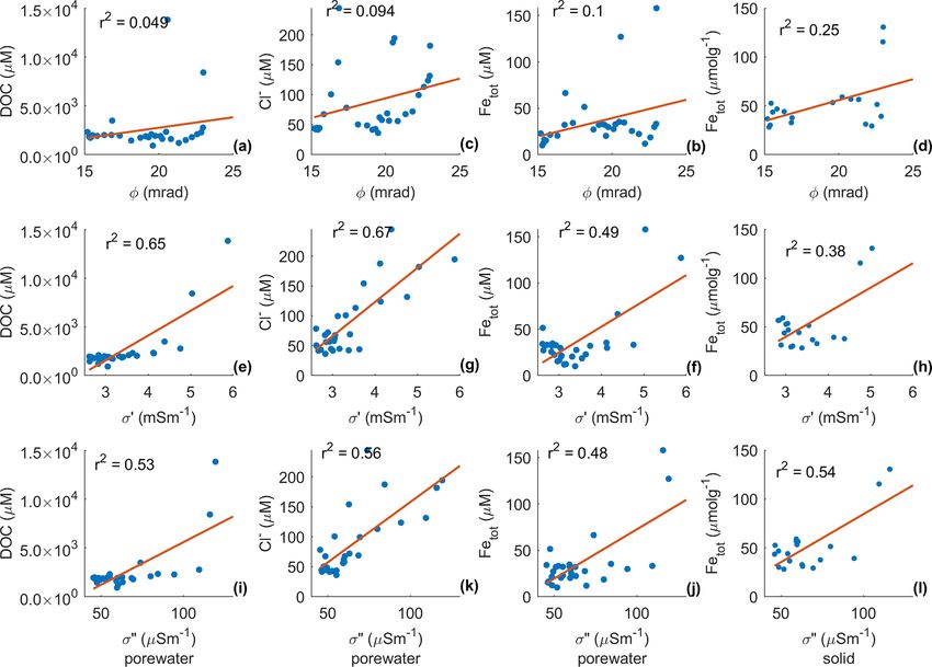
T. Katona et al.: High-resolution induced polarization imaging of biogeochemical carbon 4043
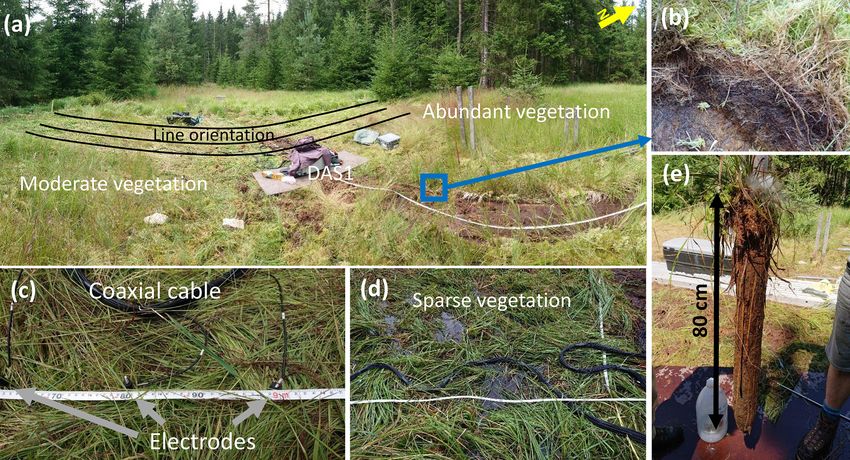
Figure 2. (a) Panoramic overview of the study site and the measurement setup. Pictures show the experimental setup and differences in the
vegetation density between the northern and southern parts of the experimental plot. The induced polarization (IP) lines appear distorted due
to the panoramic view. (b) Sphagnum in the northern part of the experimental plot. (c) Coaxial cables and stainless-steel electrodes used for
IP measurements. (d) Vegetation and the coaxial cable bundle used for IP measurements in the water-covered area in the southeastern part of
the experimental plot. (e) The freeze core shows the internal structure of the peat.
the subsurface materials. The conductivity (σ 0 ) is related to
porosity, saturation, the conductivity of the fluid filling the
pores, and a contribution of the surface conductivity (Lesmes
and Frye, 2001). The polarization (σ 00 ) is only related to
the surface conductivity taking place at the electrical double
layer (EDL) at the grain–fluid interface. For a detailed de-
scription of the IP method, the reader is referred to the work
of Ward (1988), Binley and Kemna (2005), and Binley and
Slater (2020).
The strongest polarization response is observed in the
presence of electrically conducting minerals (e.g., iron) (e.g.,
Pelton et al., 1978) in the so-called electrode polarization
(Wong et al., 1979). It arises from the different charge trans-
port mechanisms in the electrical conductor (electronic or
semiconductor conductivity) and the electrolytic conductiv-
ity of the surrounding pore fluid, which make the solid–liquid
interface polarizable. Diffusion-controlled charging and re-
Figure 3. Schematic map of the experimental plot. The solid lines laxation processes inside the grain (e.g., Revil et al., 2018,
represent the measured profiles; the bold lines represent the position 2019; Abdulsamad et al., 2019) or outside the grain in the
of the profiles discussed in this paper (By 25, By 46, and By 68).
electrolyte (e.g., Wong, 1979; Bücker et al., 2019) are con-
The arrows indicate the groundwater flow direction. The points rep-
resent the locations of fluid (S1, S2, and S3) and freeze-core (S1,
sidered possible causes of the polarization response at low
S2) samples as well as the position of piezometric tubes, where the frequencies irrespective of the specific modeling approach.
water level was measured. All mechanistic models predict an increase in the polariza-
tion response with increasing volume content of the conduc-
tive minerals (Wong, 1979; Revil et al., 2015a, b, 2017a, b,
or in terms of its magnitude (|σ |) and phase (φ): 2018; Qi et al., 2018; Bücker et al., 2018).
σ ∗ = σ 0 + iσ 00 = |σ |eiφ , (1) In the absence of electron conductors, the polarization re-
sponse is only related to the accumulation and polarization
√ p
where i = −1 is the imaginary unit, |σ | = σ 0 2 + σ 00 2 , of ions in the EDL. Different models have been proposed
and φ = tan−1 (σ 0 /σ 00 ). The real part of the complex con- to describe the polarization response as a function of grain
ductivity is mainly related to the Ohmic conduction, while size, surface area, and surface charge (e.g., Schwarz, 1962;
the imaginary part is mainly related to the polarization of Schurr, 1964; Leroy et al., 2008). Alternatively, the mem-
https://doi.org/10.5194/bg-18-4039-2021 Biogeosciences, 18, 4039–4058, 2021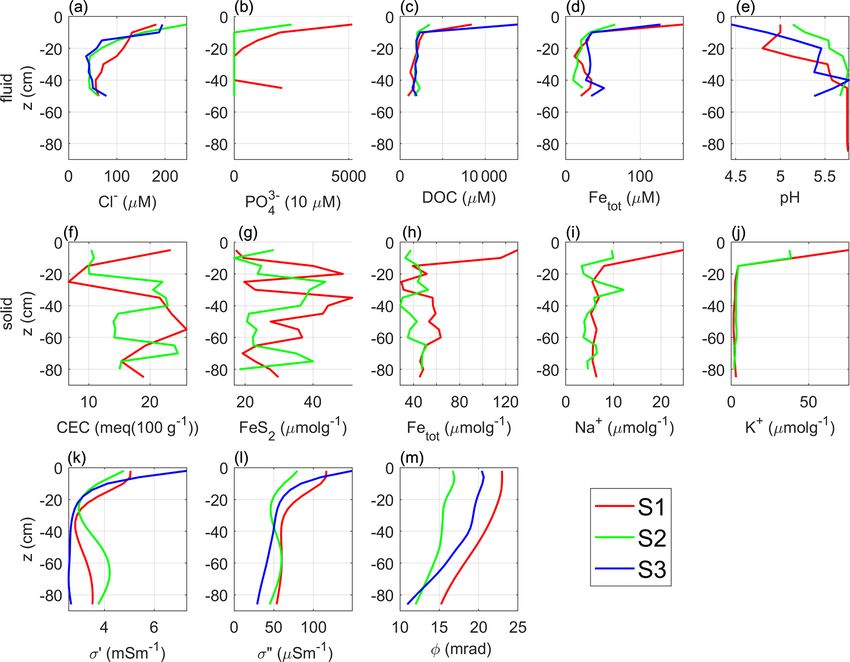
4044                             T. Katona et al.: High-resolution induced polarization imaging of biogeochemical carbon

brane polarization related the IP response to variations in the    confidence specified by an error model. We used the resis-
geometry of the pores as well as the concentration and mo-         tance and phase error models described by Kemna (2000)
bility of the ions (e.g., Marshall and Madden, 1959; Bücker        and Flores Orozco et al. (2012a). The resistance (R) error
and Hördt, 2013; Bücker et al., 2019). Regardless of the           model is expressed as s(R) = a + bR, where a is the abso-
specific modeling approach, EDL polarization mechanisms            lute error, which dominates at small resistances (i.e., R
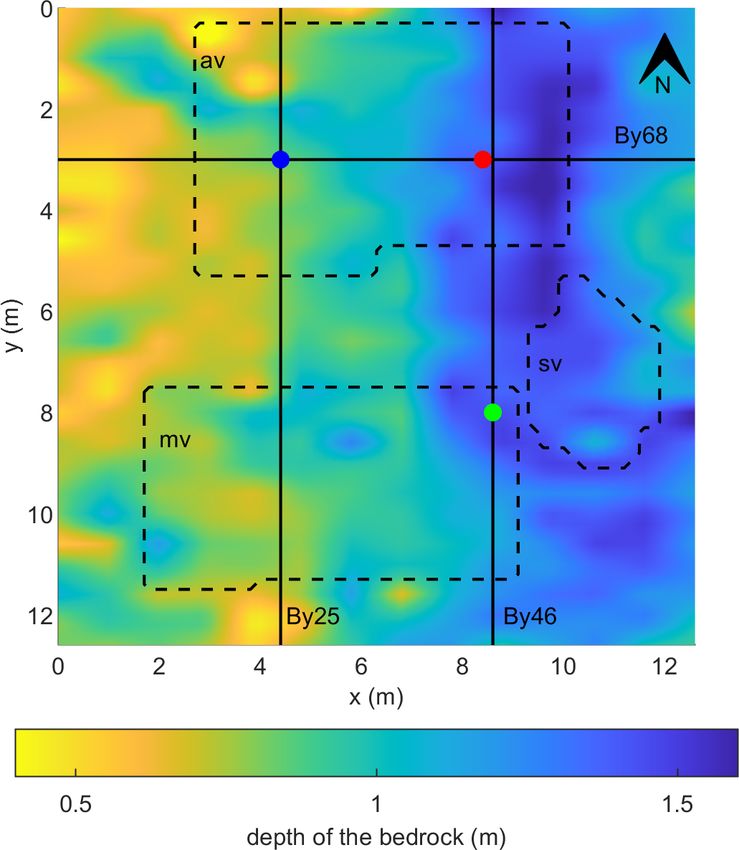
T. Katona et al.: High-resolution induced polarization imaging of biogeochemical carbon 4045
Figure 4. Raw data analysis. Raw-data pseudosections of (a) the ap-
parent resistivity and (b) the apparent phase shift for measurements
collected along profile By 25. Histograms of the normal–reciprocal Figure 5. Variations in the thickness of the peat layer, i.e., depth to
misfits of (c) the measured resistance (normalized) and (d) the ap- the granite bedrock. The positions of the three selected IP profiles
parent phase shift. By 25, By 46, and By 68 are indicated (solid lines) as well as the
position of the sampling points and the geometry of the three classes
of vegetation cover: abundant vegetation (av), moderate vegetation
Figure 6 shows the imaging results of the N–S-oriented (mv), and sparse vegetation (sv).
profiles By 25 and By 46 and the W–E-oriented profile
By 68 expressed in terms of the conductivity (σ 0 ) and po-
larization (σ 00 ). These images reveal three main electrical σ 00 /σ 0 ). Thus, it can also be used to represent the polariza-
units: (i) a shallow peat unit with high σ 0 (> 5 mSm−1 ) and tion response (Kemna et al., 2004; Ulrich and Slater, 2004;
high σ 00 (> 100 µS m−1 ) values in the top 10–20 cm b.g.s., Flores Orozco et al., 2020). Similarly to the σ 00 images, the
(ii) an intermediate unit in the peat with moderate to low phase images presented in Fig. 7 resolve the three main units:
σ 0 (< 5 mS m−1 ) and moderate σ 00 (40– 100 µS m−1 ) values, (i) the shallow peat unit within the top 10–50 cm is character-
and, (iii) underneath it, a third unit characterized by moder- ized by the highest values (φ > 18 mrad), (ii) the intermediate
ate to low σ 0 (< 5 mS m−1 ) and the lowest σ 00 (< 40 µS m−1 ) unit still corresponding to peat is characterized by moderate
values corresponding to the granite bedrock. The compact φ values (between 13 and 18 mrad), and (iii) the third unit,
structure of the granite, corresponding to low porosity, ex- associated with the granitic bedrock, is related to the lowest
plains the observed low conductivity values (σ 0 < 5 mS m−1 ) φ values (< 13 mrad). The polarization images expressed in
due to low surface charge and surface area. The shallow and terms of φ show a higher contrast between the peat and the
intermediate electrical units are related to the relatively het- granite units than the σ 0 (or σ 00 ) images. The histograms pre-
erogeneous peat (Fig. 6), which is beyond the vertical change sented in Fig. 7 show the distribution of the phase values in
and lateral heterogeneities in the complex conductivity pa- the images, with a different color for model parameters ex-
rameters. As shown in the plots of σ 00 in Fig. 6, the contact tracted above and below the contact between peat and gran-
between the second and third units roughly corresponds to ite. The histograms highlight the fact that the lowest phase
the contact between peat and granite measured with the metal values clearly correspond to the granite bedrock (< 13 mrad),
rod. This indicates the ability of IP imaging to resolve the ge- while higher phase values are characteristic of the peat unit.
ometry of the peat unit. However, for the survey design used Moreover, the shallow unit shows more pronounced lat-
in this study, σ 00 images are not sensitive to materials deeper eral variations in the phase than in σ 00 , and patterns within
than ∼ 1.25 m. Images of the electrical conductivity reveal the peat unit are more clearly defined. As observed in Fig. 6,
much more considerable variability and a lack of clear con- along line By 25, the thickness of the first unit decreases from
trasts between the peat and the granite materials, likely due approx. 0.5 m at 2 m along the profile to 0 m around 10 m
to the weathering of the shallow granite unit (Lischeid et al., at the end of the profile. Along line By 46, the first unit is
2002; Partington et al., 2013). slightly thicker than 50 cm and shows the highest phase val-
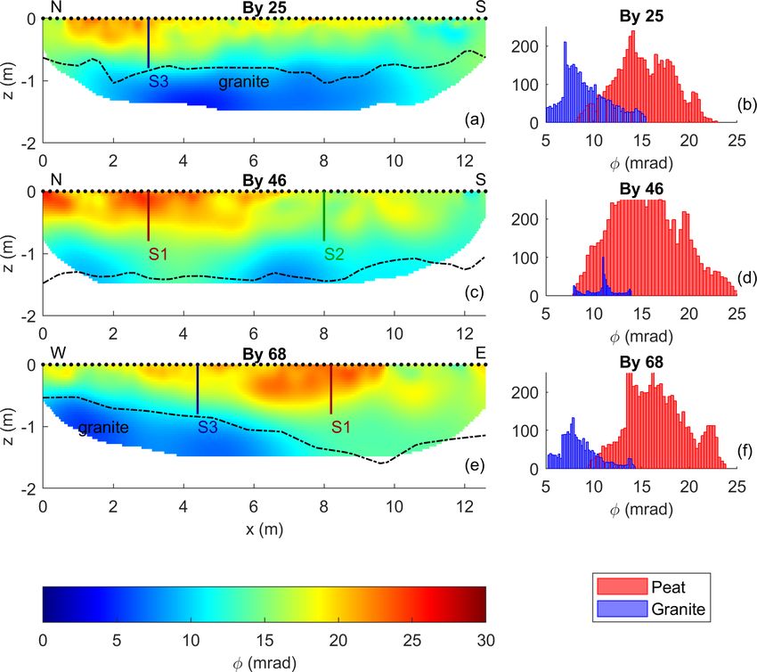
The phase of the complex conductivity represents the ra- ues (∼ 25 mrad) between 0 and 6.5 m along the profile. Be-
tio of the polarization relative to the Ohmic conduction (φ = yond 6.5 m, the polarizable unit becomes discontinuous with
https://doi.org/10.5194/bg-18-4039-2021 Biogeosciences, 18, 4039–4058, 2021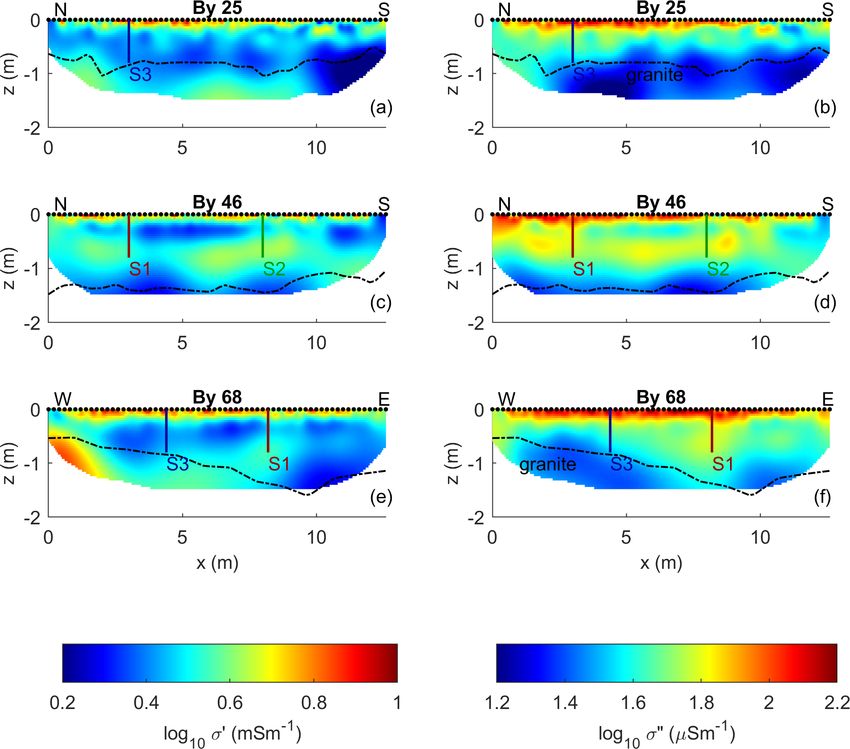
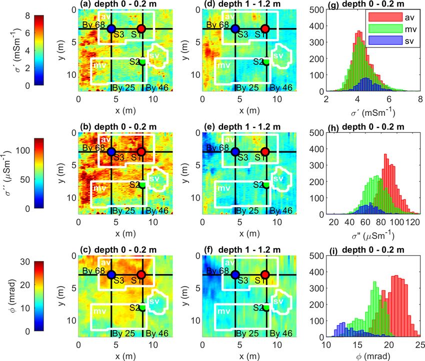
4046                               T. Katona et al.: High-resolution induced polarization imaging of biogeochemical carbon

Figure 6. Imaging results for data collected along profiles By 25 (a, b), By 46 (c, d), and By 68 (e, f) expressed as real σ 0 and imaginary
σ 00 components of the complex conductivity. The dashed lines represent the contact between the peat and granite; the black dots show the
electrode positions at the surface. The vertical lines represent the locations of the fluid (S1, S2, and S3) and freeze-core (S1, S2) samples.

isolated polarizable (∼ 18 mrad) zones, extending to a depth             tation; we observe a higher polarization response for the top
of 50 cm. The geometry of the shallow, polarizable unit is               20 cm (φ > 18 mrad and σ 00 > 80 µS m−1 ) than, for instance,
consistent with the corresponding results along line By 68,              the one corresponding to the moderate vegetation located in
which crosses By 25 and By 46 at 3 m along these lines (S1               the southern part. In contrast, the lowest polarization values
and S3 are located at these intersections). In particular, the           (φ < 15 mrad and σ 00 < 80 µS m−1 ), which we interpret as
highest phase values are consistently found in the shallow-              biogeochemically inactive zones, are related to the area with
est 50 cm in the peat unit, at the depth where biogeochemical            sparse vegetation and permanent surface runoff.
hotspots have been reported in the study by Frei et al. (2012).              Kleinebecker et al. (2009) suggest that besides climatic
   Figure 8 presents maps of the electrical parameters at dif-           variables, biogeochemical characteristics of the peat influ-
ferent depths aiming to identify lateral changes in the possi-           ence the composition of vegetation in wetlands. Hence, we
ble hotspots across the entire experimental plot. Such maps              can use variations in the vegetation as a qualitative way of
present the interpolation of values inverted in each profile.            evaluating our interpretation of the IP imaging results. In
Along each profile, a value is obtained through the average of           Fig. 8g–i, we present the histograms of the electrical parame-
model parameters (conductivity magnitude and phase) within               ters extracted at each of the three vegetation features defined
the surface and a depth of 20 cm (shallow maps) and between              in the experimental plot (abundant, moderate, and sparse).
100 and 120 cm (for deep maps). The western part of the ex-              These histograms show, in general, that the location with
perimental plot (between 0 and 4 m in the x direction and be-            sparse vegetation, i.e., with permanent surface runoff, is re-
tween 2 and 9 m in the y direction) corresponds to a shallow             lated to the lowest phase values (histogram peak at 13 mrad).
depth to the bedrock (a peat thickness of ∼ 50–70 cm) and                Moderate vegetation corresponds to moderate phase and
is associated with high electrical parameters in the shallow             σ 00 values (histogram peak at 18 mrad and 70 µS m−1 , re-
maps (φ > 18 mrad, σ 0 > 7, and σ 00 > 100 mS m−1 ), which               spectively). In comparison, the abundant vegetation corre-
we can interpret here as the geometry of the biogeochemical              sponds to the highest phase and σ 00 values (histogram peak at
hotspots. Another hotspot can be identified in the northern              22 mrad and 90 µS m−1 , respectively) in the top 20 cm. The
part of the experimental plot, in the area with abundant vege-

Biogeosciences, 18, 4039–4058, 2021                                                           https://doi.org/10.5194/bg-18-4039-2021
T. Katona et al.: High-resolution induced polarization imaging of biogeochemical carbon                                                 4047

Figure 7. Imaging results for data collected along profiles By 25 (a), By 46 (c), and By 68 (e), expressed as phase values φ of the complex
conductivity. The dashed lines represent the contact between peat and granite; the black dots show the electrode positions at the surface. The
vertical lines represent the location of the fluid (S1, S2, S3) and freeze-core (S1, S2) samples. The histograms represent the phase values of
the granite and peat extracted from the imaging results in Fig. 6b, d, f according to the geometry of the dashed lines.

histogram of the three vegetation features in terms of σ 0 val-          electrical parameters and geochemical data, Fig. 9k–m show
ues overlaps with each other.                                            the complex conductivity parameters (σ 0 , σ 00 , and φ) at the
                                                                         sampling points S1, S2, and S3, which were extracted as ver-
3.3   Comparison of electrical and geochemical                           tical 1D profiles from the corresponding imaging results.
      parameters                                                            As observed in Figs. 6 and 7, the highest complex con-
                                                                         ductivity values (σ 0 , σ 00 ) were resolved within the uppermost
The evaluations of the imaging results measured along pro-               10–20 cm and rapidly decreased with depth. Furthermore, the
files By 25, By 46, and By 68 were used to select the loca-              values of φ and σ 00 in the top 20 cm at S1 and S3 are sig-
tions for the freeze core and sampling of groundwater. Sam-              nificantly higher than those at location S2. High values of
pling points S1 and S3 were defined in the highly polarizable            φ and σ 00 at S1 and S3 correspond to high concentrations
parts of the uppermost peat unit (high σ 0 and σ 00 values). In          of DOC, phosphate, Fetot in water samples, as well as high
contrast, sampling point S2 is located in an area character-             K+ , and Na+ contents measured in soil materials extracted
ized by low polarization values. Figure 9a–e show the chem-              from the freeze cores. Figure 9 reveals consistent patterns be-
ical parameters measured in the water samples, specifically              tween geochemical and geophysical parameters: in the first
chloride (Cl− ), phosphate (PO3−4 ), dissolved organic carbon
                                                                         10 cm b.g.s. close to sampling points S1 and S3, we observe
(DOC), total iron (Fetot = Fe2+ + Fe3+ ), and pH, whereas                complex conductivity values (σ 0 and σ 00 ) as well as chem-
Fig. 9f–j show the chemical parameters measured in the peat              ical parameters, such as DOC and phosphate (only at S1).
samples extracted from the freeze cores, namely, CEC, con-               Accordingly, at S1 Fetot also reveals at least 2 times higher
centrations of iron sulfide (FeS or FeS2 ), total reactive iron          concentrations than those measured in S2.
(Fetot ), potassium (K+ ), and sodium (Na+ ). The pore-fluid                Figure 10 shows the actual correlations between the com-
conductivity measured in water samples retrieved from the                plex conductivity and Cl− , DOC, and Fetot concentrations
piezometers shows minor variation with values ranging be-                measured in groundwater samples. In Fig. 10, we also pro-
tween 6.7 and 10.4 mS m−1 . To facilitate the comparison of              vide a linear regression analysis to quantify the correlation

https://doi.org/10.5194/bg-18-4039-2021                                                           Biogeosciences, 18, 4039–4058, 2021
4048 T. Katona et al.: High-resolution induced polarization imaging of biogeochemical carbon
Figure 8. Maps of the complex conductivity at different depths. The black lines indicate the profiles By 25, By 46, and By 68. The dots
represent the locations of the vertical sampling profiles S1, S2, and S3. The white lines outline areas classified as (av) abundant vegetation,
(mv) moderate vegetation, (sv) sparse vegetation, and histograms of the complex-conductivity imaging results of the masked areas, the
abundant vegetation (red bins), the moderate vegetation (green bins), and the sparse vegetation (blue bins).
between parameters. Figure 10 reveals that the phase has a 4 Discussion
weak to moderate correlation with DOC, Cl− , and Fetot . The
conductivity (σ 0 ) shows a slightly stronger correlation with 4.1 Biogeochemical interpretation
the DOC, the Cl− , and total iron concentration than the po-
larization (σ 00 ). The highest σ 00 values (> 100 µS m−1 ) are The geochemical and geoelectrical parameters presented in
related to the highest DOC and total iron concentration. Figs. 6–7 and 9 reveal consistent patterns, with the highest
Further evidence of the presence of the biogeochemical values within the uppermost 10 cm around S1 and S3. The
hotspot interpreted at the position of S1 is available by the high DOC, K+ , and phosphate concentrations in the upper-
FTIR spectroscopy analysis of the freeze-core samples pre- most peat layers and especially in the areas found to be bio-
sented in Fig. 11. The spectra show the absorbance intensity geochemically active strongly suggest that there is rapid de-
at different wave numbers, C–O bond (∼ 1050 cm−1 ), C=O composition of dead plant material in these areas (Bragazza
double bond (∼ 1640 cm−1 ), carboxyl (∼ 1720 cm−1 ), and et al., 2009). Ions such as K+ and phosphate are essential
O–H bonds (∼ 3400 cm−1 ). The peaks are also indicated in plant nutrients, and phosphate species especially are often the
Fig. 11 with the interpretation based on the typical values re- primary limiting nutrient in peatlands (Hayati and Proctor,
ported in peatlands, for instance, McAnallen et al. (2018) or 1991). The presence of dissolved phosphate in porewaters
Artz et al. (2008). suggests that (i) the plant uptake rate of this essential nutri-
ent is exceeded by its production through the decomposition
of plant material and (ii) that organic matter turnover must
be rapid indeed to deliver this amount of phosphate to the
porewater. This is supported by the DOC concentrations in
Biogeosciences, 18, 4039–4058, 2021 https://doi.org/10.5194/bg-18-4039-2021T. Katona et al.: High-resolution induced polarization imaging of biogeochemical carbon 4049
Figure 9. Results of geochemical analyses of water and soil samples. Fluid-sample analysis of the (a) chloride Cl− , (b) phosphate PO3− 4 ,
(c) dissolved organic carbon, (d) total iron Fetot , and (e) pH. Freeze-core sample analysis of the (f) cation exchange capacity CEC, (g) iron
sulfide FeS2 , (h) total iron Fetot , (i) sodium Na+ , and (j) potassium K+ . Imaging results at the three sampling locations in terms of (k) real
component σ 0 , (l) imaginary component σ 00 , and (m) phase φ of the complex conductivity.
porewater exceeding 10 mM. DOC is produced as a decom- The high DOC concentrations are also likely to be directly
position product during microbial hydrolysis and oxidation or indirectly responsible for the Fe maximum in the upper
of solid-phase organic carbon via enzymes such as phenol layers. Dissolved Fe was predominantly found as Fe2+ (re-
oxidase (Kang et al., 2018). Enzymatic oxidation processes ducing conditions), suggesting either that high labile DOC
are enhanced by oxygen ingress via diffusion and, more im- levels maintain a low redox potential or that the dissolved
portantly, by water table fluctuations that work as an “oxy- Fe2+ was complexed with the DOC limiting the oxidation
gen pump” to the shallow subsurface (Estop-Aragonés et al., kinetics enough so that Fe2+ can accumulate in peat pore-
2012). Thus, an increased DOC concentration in the pore- waters. The TRIS analysis clearly showed very low levels of
water can be used as an indicator of microbial activity (Eli- sulfide minerals in both freeze cores, especially in the upper-
fantz et al., 2011; Liu, 2013). The small amount of phos- most peat layers. This was unexpected considering the reduc-
phate measured in the less active area S2 can be explained ing conditions implied by the dominance of porewater Fe2+ .
by advective transport from the active area S1, which is di- We argue that the lack of sulfide minerals is due to insuffi-
rectly “upstream” of S2. In this case, advective water flow cient H2 S or HS− needed to form FeS or FeS2 or that the
through the uppermost peat layers along the hydrological redox potential was not low enough to reduce sulfate to H2 S
head gradient may have transported a small amount of re- or HS− . Both mechanisms are possible, as groundwater in
action products from the biogeochemical source areas to the the catchment generally has low sulfate concentrations, and
“non-active” area. The high DOC, Fe, K+ , and phosphate yet sulfate was detected in peat porewater samples, which
(only at S1) levels confirm our initial interpretation of the would not be expected if redox potentials were low enough
highly conductive and polarizable geophysical units within to reduce sulfate to sulfide. The chemical analyses do not re-
the first 20–50 cm b.g.s. in the surroundings of S1 and S3 as veal any significant or systemic vertical gradient in mineral
biogeochemically active areas. sulfide concentrations, as expected for the site (Frei et al.,
2012). The maximum in extractable (reactive) solid-phase Fe
https://doi.org/10.5194/bg-18-4039-2021 Biogeosciences, 18, 4039–4058, 20214050 T. Katona et al.: High-resolution induced polarization imaging of biogeochemical carbon
Figure 10. Correlations between the geophysical and geochemical parameters, phase (φ), the real (σ 0 ) and imaginary (σ 00 ) components of
the complex conductivity (retrieved from the imaging results) and the biogeochemical analysis, expressed in terms of the dissolved organic
carbon (DOC), and chloride (Cl− ) content from the pore-fluid samples and total iron (Fetot ) content from pore fluid in µmol L−1 and solid
samples in µmol g−1 . The correlation coefficients of least-square regression analysis are shown in the top left corners of the subplots.
was also located in the uppermost peat layer at the “hotspot” 2001; Parikh and Chorover, 2006). Furthermore, the iron can
S1. This Fe was likely in the form of iron oxides or bound also form complexes with the carboxyl groups (absorbance
to/in the plant organic matter. Such iron-rich layers typically at ∼ 1720 cm−1 ).
form at the redox boundary between oxic and anoxic zones
and can be highly dynamic depending on variations in the 4.2 Correlation between the peat and the electrical
peatland water levels and oxygen ingress (Wang et al., 2017; signatures
Estop-Aragonés et al., 2013).
Similarly to other peatlands (Artz et al., 2008), the FTIR The two electrical units observed within the peat indicate
spectra show the presence of carbon–oxygen bonds such as variations in the biogeochemical activity with depth. Thus,
C–O, C=O, and COOH at both S1 and S2. Furthermore, the it is likely that the anomalies associated with the highest σ 0 ,
peak intensities at S1 tend to decrease with the depth, while σ 00 , and φ values in the uppermost unit correspond to the
the peak intensities at S2 samples tend to increase in agree- location of active biogeochemical zones, i.e., a hotspot. Con-
ment with the increase in the polarization response (both sequently, the moderate σ 0 , σ 00 , and φ values indicate a less
phase and σ 00 ). This observation further supports our inter- biogeochemically active or even inactive zone in the peat.
pretation of the shallow 10 cm in IP images in the vicinity The third unit represents the granitic bedrock. The low metal
of S1 as a biogeochemical hotspot. However, such a bio- content and the well-crystallized form of the granite lead to
geochemical hotspot is not related to the accumulation of low σ 00 values (here, < 40 µS m−1 ), as suggested by Marshall
iron sulfides, which was suggested by Abdel Aal and Atek- and Madden (1959).
wana (2014) or Wainwright et al. (2016) as the main param- The high polarization response of the biogeochemically
eter controlling the high IP response. The phosphate and Fe active peat (here σ 00 > 100 µS m−1 and φ > 18 mrad) is con-
could potentially form complexes with the O–H groups that sistent with the measurements of McAnallen et al. (2018),
show an absorbance peak at 1050 cm−1 (Arai and Sparks, who performed time-domain IP measurements in different
peatlands. They suggest that the active peat is less polariz-
Biogeosciences, 18, 4039–4058, 2021 https://doi.org/10.5194/bg-18-4039-2021T. Katona et al.: High-resolution induced polarization imaging of biogeochemical carbon 4051
Figure 11. Fourier transform infrared (FTIR) spectroscopy of the freeze-core samples collected at S1 (a) and S2 (b). Each sample was
extracted from the 10 cm segments. The lines represent the depth at every 10 cm between 0 and 80 cm below the ground surface. The
relevant peaks show the absorbance intensity; the interpretation is based on Artz et al. (2008), Arai and Sparks (2001), and Parikh and
Chorover (2006).
able due to the presence of the abundant sphagnum cover. 4.3 Possible polarization mechanisms
They found that in the areas where the peat is actively ac-
cumulating, the ratio of the vascular plants and the non- In this study, we have found a strong correlation between
vascular sphagnum is low and, therefore, the oxygen avail- the polarization response (φ and σ 00 ) and Fetot in the solid
ability is low. However, the sphagnum is expected to ex- phase and a less pronounced correlation between the po-
ude a small amount of carbon into the peat, and Fenner et larization response and the concentration of dissolved iron
al. (2004) found that the sphagnum contributes to the DOC in the liquid phase (see Fig. 10). In all considered mecha-
leachate to the porewater, which is contradictory to the model nistic polarization models, the phase value depends on the
of McAnallen et al. (2018). In agreement with Fenner et volumetric content of metallic particles (Wong, 1979; Revil
al. (2004), in our study, we also observe that high DOC con- 2015a, b; Bücker et al., 2018, 2019; Feng et al., 2020) and,
tent correlates with abundant sphagnum cover, which is also therefore, the phase could reveal the possible metallic con-
found in conjunction with abundant purple moor grass. In tent in the peat. If the iron in the solid phase occurred in the
this regard, recent studies have demonstrated an increase in form of highly conductive minerals, the two above correla-
the polarization response due to the accumulation of biomass tions would point to the polarization mechanism of perfect
and activity in the root system (e.g., Weigand and Kemna conductors described by Wong (1979) as a possible expla-
2017; Tsukanov and Schwartz, 2020). However, the sphag- nation for the observed response. Previous studies (e.g., Flo-
num does not have roots; thus, it cannot directly contribute res Orozco et al., 2011, 2013) attributed the polarization of
to the polarization response. McAnallen et al. (2018) suggest iron sulfides (FeS or FeS2 ) in sediments to such a polariza-
that the vascular purple moor grass can contribute to the high tion mechanism as long as sufficient Fe2+ cations are avail-
IP, as the roots transport oxygen into the deeper area, increas- able in the porewater. Such an effect has been investigated
ing the wettability and normalized chargeability of the peat. in detail by Bücker et al. (2018, 2019) regarding the changes
Derived from the results and discussion above, we delin- in the polarization response due to surface charge and reac-
eated the geometry of the hotspots. The map presented in tion currents carried by redox reactions of metal ions at the
Fig. 12 is based on the maps of phase and imaginary conduc- mineral surface. However, in the case of the present study,
tivity values at depths of 10 and 20 cm. Hotspots interpreted the lack of sulfide and the rather high pH (inferred from the
in those areas exceeded both a phase value of 18 mrad and presence of sulfate) in the porewater do not favor the pre-
imaginary conductivity of 100 µS m−1 at the same time. Be- cipitation of conductive sulfides such as pyrite. Under these
sides the geometry of the hotspots, Fig. 12 indicates that the conditions, iron would rather precipitate as iron oxide or
hotspot activity attenuates with the depth. form iron–organic matter complexes. The electrical conduc-
tivity of most iron oxides is orders of magnitude smaller than
the conductivity of sulfides (e.g., Cornell and Schwertmann,
https://doi.org/10.5194/bg-18-4039-2021 Biogeosciences, 18, 4039–4058, 20214052 T. Katona et al.: High-resolution induced polarization imaging of biogeochemical carbon Figure 12. Imaging results in terms of the imaginary component of the complex conductivity σ 00 > 100 µS m−1 and phase φ > 18 mrad, indicating the hotspot geometry at depths of (a) 10 cm and (b) 20 cm. The dots represent the locations of the vertical sampling profiles S1, S2, and S3. 1996) and is thus too low to explain an increased polarization vary in a narrow range between 5 and 25 meq kg−1 , and we based on a perfect-conductor polarization model (e.g., Wong, did not observe any correlation between CEC and changes 1979; Bücker et al., 2018, 2019; Feng et al., 2020). The only in the polarization magnitude (σ 00 , φ). Such a lack of corre- highly conductive iron oxide is magnetite, with a conductiv- lation between the polarization effect and the CEC was also ity similar to pyrite (Atekwana et al., 2016). Consequently, reported by Ponziani et al. (2011), who conducted spectral IP the presence of magnetite could explain such a polarization. measurements on a set of peat samples. Hence, the measured However, the low pH (∼ 5) typical for peat systems does not CEC is high enough to explain a rise in EDL polarization; favor the precipitation of magnetite, but rather less conduct- however, the (small) variation in CEC does not explain the ing iron (oxy)hydroxides such as ferrihydrite (Andrade et al., observed variation in the polarization magnitude. 2010; Linke and Gislason, 2018). Analysis of sediments of The pH of the pore fluid is also known to control the mag- the freeze core also did not reveal magnetite. As indicated nitude of EDL polarization; an increase in pH usually cor- by the FTIR analysis, the iron might furthermore have built responds to an increase in the polarization magnitude (e.g., complexes with the carboxyl (absorbance at ∼ 1720 cm−1 ). Skold et al., 2011). At low pH values, H+ ions occupy (neg- Such moderately conductive iron minerals or iron–organic ative) surface sites and thus reduce the net surface charge of complexes might still cause a relatively strong polarization the EDL (e.g., Hördt et al., 2016, and references therein). Our response as predicted by the polarization model developed data seem to show the opposite behavior: we found a lower by Revil et al. (2015) and Misra et al. (2016a). In this model, pH in the highly polarizable anomalies at S1 and S3 com- which attributes the polarization response to a diffuse intra- pared to site S2 (the inactive and less polarizable location), grain relaxation mechanism, the polarization magnitude is while the pH increases at depth for decreasing values in the mainly controlled by the volumetric content. In this model, polarization (both σ 00 and φ). At the same time, variations the (moderate) particle conductivity only plays a secondary in pH are within the range 4.45 and 5.77 and thus might not role (e.g., Misra et al., 2016b). be sufficiently large to control the observed changes in the The product of both surface charge density and specific polarization response. surface area can be quantified by the CEC of a material. Besides pH, pore-fluid salinity plays a significant role in As peat mainly consists of organic matter known to have a the control of EDL polarization. Laboratory measurements high CEC, even when compared to most clay minerals (e.g., on sand and sandstone samples indicated that an increase Schwartz and Furman, 2014, and references therein), the po- in salinity leads to an early increase in the imaginary con- larization of charged organic surfaces may explain the ob- ductivity, which is eventually followed by a peak and a de- served IP response. Additionally, Garcia-Artigas et al. (2020) crease at very high salinities during later stages of the ex- concluded that bioclogging due to fine particles and biofilms periments (e.g., Revil and Skold, 2011; Weller et al., 2015). increases the specific surface area and the CEC, resulting in Hördt et al. (2016) provided a possible theoretical explana- an increase in the polarization response. However, the CEC tion for this behavior: in their membrane-polarization model, values measured in samples retrieved from the freeze core salinity controls the thickness of the diffuse layer of the EDL Biogeosciences, 18, 4039–4058, 2021 https://doi.org/10.5194/bg-18-4039-2021
T. Katona et al.: High-resolution induced polarization imaging of biogeochemical carbon                                         4053

and depends on the specific geometry of the pores; there is       eas or hotspots in peatlands. Although the exact polariza-
an optimum thickness, which maximizes the magnitude of            tion mechanism is not fully understood, our results reveal
the polarization response. In the present study, we observed      that the IP response of the peat changes with the level of
that an increase in salinity (as indicated by the high Cl− con-   biogeochemical activity. Thus, the IP method is capable of
centrations within the uppermost 10 cm at all sampling loca-      distinguishing between biogeochemically active and inactive
tions) is associated with an increase in the polarization mag-    zones within the peat. The phase and imaginary conductiv-
nitude response (e.g., Revil and Skold, 2011; Weller et al.,      ity values show a contrast between these active and inactive
2015; Hördt et al., 2016). However, the highest Cl− concen-       zones and characterize the geometry of the hotspots even
trations were observed for the shallow layers at location S2,     if iron sulfides are not present. The joint interpretation of
where we measured lower polarization magnitudes (in terms         chemical and geophysical data indicates that anomalous re-
of σ 00 , φ) compared to S1 and S3.                               gions (characterized by phase values above 18 mrad and an
   The strong correlation between the polarization response       imaginary conductivity of 100 µS m−1 ) delineate the geome-
and the DOC suggests an, as yet not fully understood, causal      try of the hotspots, which are limited to the top 10 cm b.g.s.
relationship. A similar observation has recently been re-         Deeper areas (> 10 cm) of the peat are less active. In this re-
ported by Flores Orozco et al. (2020), who found a strong         gard, our study shows that the induced polarization method
correlation between the organic carbon content as a proxy         is able to characterize biogeochemical changes and their ge-
of microbial activity and both σ 0 and σ 00 in a municipal        ometry within peat with high resolution. Additionally, our
waste landfill in Austria. Regarding the available carbon,        study demonstrates the ability of the IP method to map bio-
McAnallen et al. (2018) reported a strong correlation be-         geochemically active zones even if they are not related to the
tween the occurrence of long-chained C=O double bonds and         microbiologically mediated accumulation of iron sulfides.
the total chargeability of peat material. The upper peat layers   We identify complexes of organic matter and iron as pos-
are exposed to oxygen, leading to oxidation of the peat and       sible causes of the high polarization response of the carbon
formation of C=O double bonds at solid-phase surfaces and         turnover hotspots investigated in our study. Further labora-
in the porewater DOC. Such long-chained organic molecules         tory studies on peat samples with different concentrations
have an increased wettability and thus more readily attach (or    and mixtures of DOC, phosphate, and iron in the pore fluid
even form at organic matter surfaces) to the surface of solid     are required to fully understand the effect in IP signatures due
organic and mineral particles (Alonso et al., 2009). Based on     to iron–organic complexes and the control phosphate exerts
a membrane-polarization model, Bücker et al. (2017) predict       over the related polarization process.
an increase in the polarization magnitude in the presence of
wetting (i.e., long-chained) hydrocarbon in the free phase.
The long-chained polar DOC attaches to the peat surface,          Data availability. All data are available from the corresponding au-
similarly to polar hydrocarbon, and so it might provide ex-       thor upon request.
tra surface charge, thus reducing the pore space and causing
membrane polarization (Marshall and Madden, 1959).
   As suggested by Vindedahl et al. (2016), organic mat-          Author contributions. AFO and TK designed the experimental
ter can adsorb to the iron-oxide surface via electrostatic at-    setup, and TK conducted the field survey and analysis of the geo-
                                                                  physical data. BSG and SF conducted the geochemical measure-
traction and provides a negatively charged macromolecu-
                                                                  ments and their interpretation. AFO, MB, and TK interpreted the
lar layer on the iron oxide. Such complexes could also ex-
                                                                  geophysical signatures. TK lead the preparation of the draft, where
plain the observed increase in the polarization response in       SF, BSG, MB, and AFO contributed equally.
the anomalies interpreted as biogeochemical hotspots. The
point of zero charge of the peat is below pH 4 (Bakatula et
al., 2018), while for iron (oxide) it varies between ∼ 5 and      Competing interests. The authors declare that they have no conflict
∼ 9 (Kosmulski et al., 2003). This means that the organic         of interest.
matter is probably negatively charged, and the iron oxide is
most likely positively charged since the measured pH at the
sample points varies between 4.5 and 5.8, with lower values       Disclaimer. Publisher’s note: Copernicus Publications remains
in the top 10 cm in the hotspot area. Hence, in the shallow       neutral with regard to jurisdictional claims in published maps and
10 cm from S1 and S3, the pH favors the DOC to bond with          institutional affiliations.
the iron in the solid phase.

                                                                  Acknowledgements. This research was supported by German Re-
5   Conclusions                                                   search Foundation (DFG) projects FR 2858/2-1-3013594 and GI
                                                                  792/2-1. The work of Timea Katona was supported by the Explo-
                                                                  GRAF project (development of geophysical methods for the explo-
We investigated the applicability of induced polarization (IP)
                                                                  ration of graphite ores) funded by the Austrian Federal Ministry of
as a tool to identify and localize biogeochemically active ar-

https://doi.org/10.5194/bg-18-4039-2021                                                    Biogeosciences, 18, 4039–4058, 2021
You can also read