Information from Paleoclimate Archives - IPCC
←
→
Page content transcription
If your browser does not render page correctly, please read the page content below
Information from
    Paleoclimate Archives
5   Coordinating Lead Authors:
    Valérie Masson-Delmotte (France), Michael Schulz (Germany)

    Lead Authors:
    Ayako Abe-Ouchi (Japan), Jürg Beer (Switzerland), Andrey Ganopolski (Germany), Jesus Fidel
    González Rouco (Spain), Eystein Jansen (Norway), Kurt Lambeck (Australia), Jürg Luterbacher
    (Germany), Tim Naish (New Zealand), Timothy Osborn (UK), Bette Otto-Bliesner (USA), Terrence
    Quinn (USA), Rengaswamy Ramesh (India), Maisa Rojas (Chile), XueMei Shao (China), Axel
    Timmermann (USA)

    Contributing Authors:
    Kevin Anchukaitis (USA), Julie Arblaster (Australia), Patrick J. Bartlein (USA), Gerardo Benito
    (Spain), Peter Clark (USA), Josefino C. Comiso (USA), Thomas Crowley (UK), Patrick De Deckker
    (Australia), Anne de Vernal (Canada), Barbara Delmonte (Italy), Pedro DiNezio (USA), Trond
    Dokken (Norway), Harry J. Dowsett (USA), R. Lawrence Edwards (USA), Hubertus Fischer
    (Switzerland), Dominik Fleitmann (UK), Gavin Foster (UK), Claus Fröhlich (Switzerland), Aline
    Govin (Germany), Alex Hall (USA), Julia Hargreaves (Japan), Alan Haywood (UK), Chris Hollis
    (New Zealand), Ben Horton (USA), Masa Kageyama (France), Reto Knutti (Switzerland), Robert
    Kopp (USA), Gerhard Krinner (France), Amaelle Landais (France), Camille Li (Norway/Canada),
    Dan Lunt (UK), Natalie Mahowald (USA), Shayne McGregor (Australia), Gerald Meehl (USA),
    Jerry X. Mitrovica (USA/Canada), Anders Moberg (Sweden), Manfred Mudelsee (Germany),
    Daniel R. Muhs (USA), Stefan Mulitza (Germany), Stefanie Müller (Germany), James Overland
    (USA), Frédéric Parrenin (France), Paul Pearson (UK), Alan Robock (USA), Eelco Rohling
    (Australia), Ulrich Salzmann (UK), Joel Savarino (France), Jan Sedláček (Switzerland), Jeremy
    Shakun (USA), Drew Shindell (USA), Jason Smerdon (USA), Olga Solomina (Russian Federation),
    Pavel Tarasov (Germany), Bo Vinther (Denmark), Claire Waelbroeck (France), Dieter Wolf-
    Gladrow (Germany), Yusuke Yokoyama (Japan), Masakazu Yoshimori (Japan), James Zachos
    (USA), Dan Zwartz (New Zealand)

    Review Editors:
    Anil K. Gupta (India), Fatemeh Rahimzadeh (Iran), Dominique Raynaud (France), Heinz Wanner
    (Switzerland)

    This chapter should be cited as:
    Masson-Delmotte, V., M. Schulz, A. Abe-Ouchi, J. Beer, A. Ganopolski, J.F. González Rouco, E. Jansen, K. Lambeck,
    J. Luterbacher, T. Naish, T. Osborn, B. Otto-Bliesner, T. Quinn, R. Ramesh, M. Rojas, X. Shao and A. Timmermann,
    2013: Information from Paleoclimate Archives. In: Climate Change 2013: The Physical Science Basis. Contribution
    of Working Group I to the Fifth Assessment Report of the Intergovernmental Panel on Climate Change [Stocker,
    T.F., D. Qin, G.-K. Plattner, M. Tignor, S.K. Allen, J. Boschung, A. Nauels, Y. Xia, V. Bex and P.M. Midgley (eds.)].
    Cambridge University Press, Cambridge, United Kingdom and New York, NY, USA.
                                                                                                                            383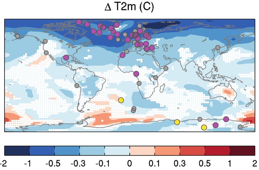
Table of Contents

    Executive Summary...................................................................... 385             5.8       Paleoclimate Perspective on Irreversibility in
                                                                                                            		        the Climate System.......................................................... 433
    5.1      Introduction....................................................................... 388            5.8.1            Ice Sheets................................................................... 433
                                                                                                                5.8.2            Ocean Circulation...................................................... 433
    5.2      Pre-Industrial Perspective on Radiative
    		       Forcing Factors.................................................................. 388              5.8.3            Next Glacial Inception................................................ 435

        5.2.1          External Forcings........................................................ 388
                                                                                                            5.9       Concluding Remarks........................................................ 435
     5.2.2             Radiative Perturbations from Greenhouse Gases
    			                and Dust.................................................................... 391
                                                                                                            References .................................................................................. 436
        Box 5.1: Polar Amplification...................................................... 396
                                                                                                            Appendix 5.A: Additional Information on Paleoclimate
    5.3      Earth System Responses and Feedbacks at                                                        Archives and Models................................................................... 456
    		       Global and Hemispheric Scales.................................... 398
        5.3.1          High-Carbon Dioxide Worlds and Temperature.......... 398                             Frequently Asked Questions
        5.3.2          Glacial–Interglacial Dynamics.................................... 399                 FAQ 5.1             Is the Sun a Major Driver of Recent Changes
                                                                                                            			                  in Climate?............................................................... 392
        Box 5.2: Climate-Ice Sheet Interactions.................................. 402
                                                                                                             FAQ 5.2             How Unusual is the Current Sea Level Rate
     5.3.3             Last Glacial Maximum and Equilibrium                                                 			                  of Change?............................................................... 430
    			                Climate Sensitivity..................................................... 403
        5.3.4          Past Interglacials........................................................ 407
     5.3.5             Temperature Variations During the
    			                Last 2000 Years.......................................................... 409

    5.4      Modes of Climate Variability........................................ 415
        5.4.1          Tropical Modes........................................................... 415
        5.4.2          Extratropical Modes................................................... 415

    5.5      Regional Changes During the Holocene................... 417
        5.5.1          Temperature............................................................... 417
        5.5.2          Sea Ice....................................................................... 420
        5.5.3          Glaciers...................................................................... 421
5       5.5.4          Monsoon Systems and Convergence Zones............... 421
        5.5.5          Megadroughts and Floods......................................... 422

    5.6      Past Changes in Sea Level............................................. 425
        5.6.1          Mid-Pliocene Warm Period......................................... 425
        5.6.2          The Last Interglacial................................................... 425
        5.6.3          Last Glacial Termination and Holocene...................... 428

    5.7      Evidence and Processes of Abrupt
    		       Climate Change................................................................ 432

    384
Information from Paleoclimate Archives                                                                                                                               Chapter 5

Executive Summary                                                                          CO2 concentrations between 350 ppm and 450 ppm (medium confi-
                                                                                           dence) occurred when global mean surface temperatures were 1.9°C
Greenhouse-Gas Variations and Past Climate Responses                                       to 3.6°C (medium confidence) higher than for pre-industrial climate
                                                                                           {5.3.1}. During the Early Eocene (52 to 48 million years ago), atmos-
It is a fact that present-day (2011) concentrations of the atmos-                          pheric CO2 concentrations exceeded ~1000 ppm (medium confidence)
pheric greenhouse gases (GHGs) carbon dioxide (CO2), methane                               when global mean surface temperatures were 9°C to 14°C (medium
(CH4) and nitrous oxide (N2O) exceed the range of concentra-                               confidence) higher than for pre-industrial conditions. {5.3.1}
tions recorded in ice cores during the past 800,000 years. Past
changes in atmospheric GHG concentrations can be determined with                           New temperature reconstructions and simulations of past
very high confidence1 from polar ice cores. Since AR4 these records                        climates show with high confidence polar amplification in
have been extended from 650,000 years to 800,000 years ago. {5.2.2}                        response to changes in atmospheric CO2 concentration. For high
                                                                                           CO2 climates such as the Early Eocene (52 to 48 million years ago) or
With very high confidence, the current rates of CO2, CH4 and N2O                           mid-Pliocene (3.3 to 3.0 million years ago), and low CO2 climates such
rise in atmospheric concentrations and the associated radiative                            as the Last Glacial Maximum (21,000 to 19,000 years ago), sea sur-
forcing are unprecedented with respect to the highest resolu-                              face and land surface air temperature reconstructions and simulations
tion ice core records of the last 22,000 years. There is medium                            show a stronger response to changes in atmospheric GHG concentra-
confidence that the rate of change of the observed GHG rise is also                        tions at high latitudes as compared to the global average. {Box 5.1,
unprecedented compared with the lower resolution records of the past                       5.3.1, 5.3.3}
800,000 years. {5.2.2}
                                                                                           Global Sea Level Changes During Past Warm Periods
There is high confidence that changes in atmospheric CO2 con-
centration play an important role in glacial–interglacial cycles.                          The current rate of global mean sea level change, starting in the
Although the primary driver of glacial–interglacial cycles lies in the                     late 19th-early 20th century, is, with medium confidence, unu-
seasonal and latitudinal distribution of incoming solar energy driven by                   sually high in the context of centennial-scale variations of the
changes in the geometry of the Earth’s orbit around the Sun (“orbital                      last two millennia. The magnitude of centennial-scale global mean
forcing”), reconstructions and simulations together show that the full                     sea level variations did not exceed 25 cm over the past few millennia
magnitude of glacial–interglacial temperature and ice volume changes                       (medium confidence). {5.6.3}
cannot be explained without accounting for changes in atmospher-
ic CO2 content and the associated climate feedbacks. During the last                       There is very high confidence that the maximum global mean
deglaciation, it is very likely2 that global mean temperature increased                    sea level during the last interglacial period (129,000 to 116,000
by 3°C to 8°C. While the mean rate of global warming was very likely                       years ago) was, for several thousand years, at least 5 m higher
0.3°C to 0.8°C per thousand years, two periods were marked by faster                       than present and high confidence that it did not exceed 10 m
warming rates, likely between 1°C and 1.5°C per thousand years,                            above present. The best estimate is 6 m higher than present. Based
although regionally and on shorter time scales higher rates may have                       on ice sheet model simulations consistent with elevation changes
occurred. {5.3.2}                                                                          derived from a new Greenland ice core, the Greenland ice sheet very
                                                                                           likely contributed between 1.4 and 4.3 m sea level equivalent, implying
New estimates of the equilibrium climate sensitivity based on                              with medium confidence a contribution from the Antarctic ice sheet
reconstructions and simulations of the Last Glacial Maximum                                to the global mean sea level during the last interglacial period. {5.6.2}
(21,000 years to 19,000 years ago) show that values below 1°C
as well as above 6°C for a doubling of atmospheric CO2 concen-                             There is high confidence that global mean sea level was above                              5
tration are very unlikely. In some models climate sensitivity differs                      present during some warm intervals of the mid-Pliocene (3.3
between warm and cold climates because of differences in the rep-                          to 3.0 million years ago), implying reduced volume of polar ice
resentation of cloud feedbacks. {5.3.3}                                                    sheets. The best estimates from various methods imply with high con-
                                                                                           fidence that sea level has not exceeded +20 m during the warmest
With medium confidence, global mean surface temperature                                    periods of the Pliocene, due to deglaciation of the Greenland and West
was significantly above pre-industrial levels during several past                          Antarctic ice sheets and areas of the East Antarctic ice sheet. {5.6.1}
periods characterised by high atmospheric CO2 concentrations.
During the mid-Pliocene (3.3 to 3.0 million years ago), atmospheric

1   In this Report, the following summary terms are used to describe the available evidence: limited, medium, or robust; and for the degree of agreement: low, medium, or high.
    A level of confidence is expressed using five qualifiers: very low, low, medium, high, and very high, and typeset in italics, e.g., medium confidence. For a given evidence and
    agreement statement, different confidence levels can be assigned, but increasing levels of evidence and degrees of agreement are correlated with increasing confidence (see
    Section 1.4 and Box TS.1 for more details).
2   In this Report, the following terms have been used to indicate the assessed likelihood of an outcome or a result: Virtually certain 99–100% probability, Very likely 90–100%,
    Likely 66–100%, About as likely as not 33–66%, Unlikely 0–33%, Very unlikely 0–10%, Exceptionally unlikely 0–1%. Additional terms (Extremely likely: 95–100%, More likely
    than not >50–100%, and Extremely unlikely 0–5%) may also be used when appropriate. Assessed likelihood is typeset in italics, e.g., very likely (see Section 1.4 and Box TS.1
    for more details).

                                                                                                                                                                              385
Chapter 5                                                                                               Information from Paleoclimate Archives

    Observed Recent Climate Change in the Context of                           late 20th century. With high confidence, these regional warm peri-
    Interglacial Climate Variability                                           ods were not as synchronous across regions as the warming since the
                                                                               mid-20th century. Based on the comparison between reconstructions
    New temperature reconstructions and simulations of the warm-               and simulations, there is high confidence that not only external orbit-
    est millennia of the last interglacial period (129,000 to 116,000          al, solar and volcanic forcing, but also internal variability, contributed
    years ago) show with medium confidence that global mean                    substantially to the spatial pattern and timing of surface temperature
    annual surface temperatures were never more than 2°C higher                changes between the Medieval Climate Anomaly and the Little Ice Age
    than pre-industrial. High latitude surface temperature, averaged over      (1450 to 1850). {5.3.5.3, 5.5.1}
    several thousand years, was at least 2°C warmer than present (high
    confidence). Greater warming at high latitudes, seasonally and annu-       There is high confidence for droughts during the last millennium
    ally, confirm the importance of cryosphere feedbacks to the seasonal       of greater magnitude and longer duration than those observed
    orbital forcing. During these periods, atmospheric GHG concentrations      since the beginning of the 20th century in many regions. There
    were close to the pre-industrial level. {5.3.4, Box 5.1}                   is medium confidence that more megadroughts occurred in monsoon
                                                                               Asia and wetter conditions prevailed in arid Central Asia and the South
    There is high confidence that annual mean surface warming                  American monsoon region during the Little Ice Age (1450 to 1850)
    since the 20th century has reversed long-term cooling trends               compared to the Medieval Climate Anomaly (950 to 1250). {5.5.4 and
    of the past 5000 years in mid-to-high latitudes of the Northern            5.5.5}
    Hemisphere (NH). New continental- and hemispheric-scale annual
    surface temperature reconstructions reveal multi-millennial cooling        With high confidence, floods larger than those recorded since
    trends throughout the past 5000 years. The last mid-to-high latitude       1900 occurred during the past five centuries in northern and
    cooling trend persisted until the 19th century, and can be attributed      central Europe, western Mediterranean region and eastern Asia.
    with high confidence to orbital forcing, according to climate model        There is medium confidence that modern large floods are comparable
    simulations. {5.5.1}                                                       to or surpass historical floods in magnitude and/or frequency in the
                                                                               Near East, India and central North America. {5.5.5}
    There is medium confidence from reconstructions that the cur-
    rent (1980–2012) summer sea ice retreat was unprecedented                  Past Changes in Climate Modes
    and sea surface temperatures in the Arctic were anomalously
    high in the perspective of at least the last 1450 years. Lower than        New results from high-resolution coral records document with
    late 20th century summer Arctic sea ice cover is reconstructed and sim-    high confidence that the El Niño-Southern Oscillation (ENSO)
    ulated for the period between 8000 and 6500 years ago in response to       system has remained highly variable throughout the past 7000
    orbital forcing. {5.5.2}                                                   years, showing no discernible evidence for an orbital modula-
                                                                               tion of ENSO. This is consistent with the weak reduction in mid-Hol-
    There is high confidence that minima in NH extratropical glacier           ocene ENSO amplitude of only 10% simulated by the majority of cli-
    extent between 8000 and 6000 years ago were primarily due                  mate models, but contrasts with reconstructions reported in AR4 that
    to high summer insolation (orbital forcing). The current glacier           showed a reduction in ENSO variance during the first half of the Hol-
    retreat occurs within a context of orbital forcing that would be favour-   ocene. {5.4.1}
    able for NH glacier growth. If glaciers continue to reduce at current
    rates, most extratropical NH glaciers will shrink to their minimum         With high confidence, decadal and multi-decadal changes in the
    extent, which existed between 8000 and 6000 years ago, within this         winter North Atlantic Oscillation index (NAO) observed since
5   century (medium confidence). {5.5.3}                                       the 20th century are not unprecedented in the context of the
                                                                               past 500 years. Periods of persistent negative or positive winter NAO
    For average annual NH temperatures, the period 1983–2012                   phases, similar to those observed in the 1960s and 1990 to 2000s,
    was very likely the warmest 30-year period of the last 800 years           respectively, are not unusual in the context of NAO reconstructions
    (high confidence) and likely the warmest 30-year period of the             during at least the past 500 years. {5.4.2}
    last 1400 years (medium confidence). This is supported by com-
    parison of instrumental temperatures with multiple reconstructions         The increase in the strength of the observed summer Southern
    from a variety of proxy data and statistical methods, and is consistent    Annular Mode since 1950 has been anomalous, with medium
    with AR4. In response to solar, volcanic and anthropogenic radiative       confidence, in the context of the past 400 years. No similar spa-
    changes, climate models simulate multi-decadal temperature changes         tially coherent multi-decadal trend can be detected in tree-ring indices
    over the last 1200 years in the NH, that are generally consistent in       from New Zealand, Tasmania and South America. {5.4.2}
    magnitude and timing with reconstructions, within their uncertainty
    ranges. {5.3.5}                                                            Abrupt Climate Change and Irreversibility

    Continental-scale surface temperature reconstructions show,                With high confidence, the interglacial mode of the Atlantic
    with high confidence, multi-decadal periods during the Medie-              Ocean meridional overturning circulation (AMOC) can recover
    val Climate Anomaly (950 to 1250) that were in some regions as             from a short-term freshwater input into the subpolar North
    warm as in the mid-20th century and in others as warm as in the            Atlantic. Approximately 8200 years ago, a sudden freshwater release

    386
Information from Paleoclimate Archives                                     Chapter 5

occurred during the final stages of North America ice sheet melting.
Paleoclimate observations and model results indicate, with high con-
fidence, a marked reduction in the strength of the AMOC followed by
a rapid recovery, within approximately 200 years after the perturba-
tion. {5.8.2}

Confidence in the link between changes in North Atlantic climate
and low-latitude precipitation patterns has increased since AR4.
From new paleoclimate reconstructions and modelling studies, there is
very high confidence that reduced AMOC and the associated surface
cooling in the North Atlantic region caused southward shifts of the
Atlantic Intertropical Convergence Zone, and also affected the Ameri-
can (North and South), African and Asian monsoon systems. {5.7}

It is virtually certain that orbital forcing will be unable to trig-
ger widespread glaciation during the next 1000 years. Paleo-
climate records indicate that, for orbital configurations close to the
present one, glacial inceptions only occurred for atmospheric CO2
concentrations significantly lower than pre-industrial levels. Climate
models simulate no glacial inception during the next 50,000 years if
CO2 concentrations remain above 300 ppm. {5.8.3, Box 6.2}

There is high confidence that the volumes of the Greenland and
West Antarctic ice sheets were reduced during periods of the
past few million years that were globally warmer than pres-
ent. Ice sheet model simulations and geological data suggest that the
West Antarctic ice sheet is very sensitive to subsurface Southern Ocean
warming and imply with medium confidence a West Antarctic ice sheet
retreat if atmospheric CO2 concentration stays within or above the
range of 350 ppm to 450 ppm for several millennia. {5.3.1, 5.6.1, 5.8.1}

                                                                                       5

                                                                                387
Chapter 5 Information from Paleoclimate Archives
5.1 Introduction Additional information to this chapter is available in the Appendix. Pro-
cessed data underlying the figures are stored in the PANGAEA data-
This chapter assesses the information on past climate obtained prior to base (www.pangaea.de), while model output from PMIP3 is available
the instrumental period. The information is based on data from various from pmip3.lsce.ipsl.fr. In all sections, information is structured by time,
paleoclimatic archives and on modelling of past climate, and updates going from past to present. Table 5.1 summarizes the past periods
Chapter 6 of AR4 of IPCC Working Group I (Jansen et al., 2007). assessed in the subsections.
The Earth system has responded and will continue to respond to
various external forcings (solar, volcanic and orbital) and to changes 5.2 Pre-Industrial Perspective on Radiative
in atmospheric composition. Paleoclimate data and modelling pro- Forcing Factors
vide quantitative information on the Earth system response to these
forcings. Paleoclimate information facilitates understanding of Earth 5.2.1 External Forcings
system feedbacks on time scales longer than a few centuries, which
cannot be evaluated from short instrumental records. Past climate 5.2.1.1 Orbital Forcing
changes also document transitions between different climate states,
including abrupt events, which occurred on time scales of decades to The term ‘orbital forcing’ is used to denote the incoming solar radiation
a few centuries. They inform about multi-centennial to millennial base- changes originating from variations in the Earth’s orbital parameters
line variability, against which the recent changes can be compared to as well as changes in its axial tilt. Orbital forcing is well known from
assess whether or not they are unusual. precise astronomical calculations for the past and future (Laskar et
al., 2004). Changes in eccentricity, longitude of perihelion (related to
Major progress since AR4 includes the acquisition of new and more precession) and axial tilt (obliquity) (Berger and Loutre, 1991) predom-
precise information from paleoclimate archives, the synthesis of inantly affect the seasonal and latitudinal distribution and magnitude
regional information, and Paleoclimate Modelling Intercomparison of solar energy received at the top of the atmosphere (AR4, Box 6.1;
Project Phase III (PMIP3) and Coupled Model Intercomparison Project Jansen et al., 2007), and the durations and intensities of local seasons.
Phase 5 (CMIP5) simulations using the same models as for projections Obliquity also modulates the annual mean insolation at any given
(see Chapter 1). This chapter assesses the understanding of past cli- latitude, with opposite effects at high and low latitudes. Orbital forc-
mate variations, using paleoclimate reconstructions as well as climate ing is considered the pacemaker of transitions between glacials and
models of varying complexity, while the model evaluation based on interglacials (high confidence), although there is still no consensus on
paleoclimate information is covered in Chapter 9. Additional paleo- exactly how the different physical processes influenced by insolation
climate perspectives are included in Chapters 6, 10 and 13 (see Table changes interact to influence ice sheet volume (Box 5.2; Section 5.3.2).
5.1). The different orbital configurations make each glacial and interglacial
period unique (Yin and Berger, 2010; Tzedakis et al., 2012a). Multi-mil-
The content of this chapter is largely restricted to topics for which sub- lennial trends of temperature, Arctic sea ice and glaciers during the
stantial new information has emerged since AR4. Examples include current interglacial period, and specifically the last 2000 years, have
proxy-based estimates of the atmospheric carbon dioxide (CO2) con- been related to orbital forcing (Section 5.5).
tent during the past ~65 million years (Section 5.2.2) and magnitude
of sea level variations during interglacial periods (Section 5.6.2). Infor- 5.2.1.2 Solar Forcing
mation from glacial climates has been included only if the underlying
processes are of direct relevance for an assessment of projected cli- Solar irradiance models (e.g., Wenzler et al., 2005) have been improved
5 mate change. The impacts of past climate changes on biological sys- to explain better the instrumental measurements of total solar irradi-
tems and past civilizations are not covered, as these topics are beyond ance (TSI) and spectral (wavelength dependent) solar irradiance (SSI).
the scope of Working Group I. Typical changes measured over an 11-year solar cycle are 0.1% for TSI
and up to several percent for the ultraviolet (UV) part of SSI (see Sec-
The chapter proceeds from evidence for pre-industrial changes in tion 8.4). Changes in TSI directly impact the Earth’s surface (see solar
atmospheric composition and external solar and volcanic forcings Box 10.2), whereas changes in UV primarily affect the stratosphere, but
(Section 5.2, FAQ 5.1), to global and hemispheric responses (Section can influence the tropospheric circulation through dynamical coupling
5.3). After evaluating the evidence for past changes in climate modes (Haigh, 1996). Most models attribute all TSI and SSI changes exclusively
of variability (Section 5.4), a specific focus is given to regional changes to magnetic phenomena at the solar surface (sunspots, faculae, mag-
in temperature, cryosphere and hydroclimate during the current inter- netic network), neglecting any potential internal phenomena such as
glacial period (Section 5.5). Sections on sea level change (Section 5.6, changes in energy transport (see also Section 8.4). The basic concept in
FAQ 5.2), abrupt climate changes (Section 5.7) and illustrations of irre- solar models is to divide the solar surface into different magnetic fea-
versibility and recovery time scales (Section 5.8) conclude the chapter. tures each with a specific radiative flux. The balance of contrasting dark
While polar amplification of temperature changes is addressed in Box sunspots and bright faculae and magnetic network leads to a higher TSI
5.1, the relationships between ice sheets, sea level, atmospheric CO2 value during solar cycle maxima and at most wavelengths, but some
concentration and climate are addressed in several sections (Box 5.2, wavelengths may be out of phase with the solar cycle (Harder et al.,
Sections 5.3.1, 5.5, and 5.8.1). 2009; Cahalan et al., 2010; Haigh et al., 2010). TSI and SSI are calculated
by adding the radiative fluxes of all features plus the contribution from
388Information from Paleoclimate Archives Chapter 5
Table 5.1 | Summary of past periods for which climate information is assessed in the various sections of this chapter and other chapters of AR5. Calendar ages are expressed
in Common Era (CE), geological ages are expressed in thousand years (ka) or million years (Ma) before present (BP), with present defined as 1950. Radiocarbon-based ages are
quoted as the published calibrated ages.
Chapter 5 Sections Other
Time Period Age
5.2 5.3 5.4 5.5 5.6 5.7 5.8 Chapters
Holocenea 11.65 kag to present 6, 9, 10
Pre-industrial period refers to times before 1850 or 1850 valuesh
Little Ice Age (LIA) 1450–1850i 10
Medieval Climate Anomaly (MCA) b
950–1250i 10
Last Millennium 1000–1999j 9, 10
Mid-Holocene (MH) ~6 ka 9, 13
8.2-ka event ~8.2 kag
Last Glacial Terminationc 6
Younger Dryasd 12.85–11.65 kag 6
Bølling-Allerøde 14.64–12.85 kag 6
Meltwater Pulse 1A (MWP-1A) 14.65–14.31 ka k
Heinrich stadial 1 (HS1) ~19–14.64 kal
Last Glacial Maximum (LGM) ~21–19 ka m
6, 9
Last Interglacial (LIG)f ~129–116 kan 13
Mid-Pliocene Warm Period (MPWP) ~3.3–3.0 Ma o
13
Early Eocene Climatic Optimum (EECO) ~52–50 Map
Paleocene-Eocene Thermal Maximum (PETM) ~55.5–55.3 Maq
Notes:
a
Also known as Marine Isotopic Stage (MIS) 1 or current interglacial.
b
Also known as Medieval Climate Optimum or the Medieval Warm Period.
c Also known as Termination I or the Last Deglaciation. Based on sea level, Last Glacial Termination occurred between ~19 and ~6 ka.
d
Also known as Greenland Stadial GS-1.
e Also known as Greenland Interstadial GI-a-c-e.
f
Also known as MIS5e, which overlaps with the Eemian (Shackleton et al., 2003).
g
As estimated from the Greenland ice core GICC05 chronology (Rasmussen et al., 2006; Thomas et al., 2007).
h In this chapter, when referring to comparison of radiative forcing or climate variables, pre-industrial refers to 1850 values in accordance with Taylor et al. (2012). Otherwise it refers to an extended
period of time before 1850 as stated in the text. Note that Chapter 7 uses 1750 as the reference pre-industrial period.
i Different durations are reported in the literature. In Section 5.3.5, time intervals 950–1250 and 1450–1850 are used to calculate Northern Hemisphere temperature anomalies representative of
the MCA and LIA, respectively.
j
Note that CMIP5 “Last Millennium simulations” have been performed for the period 850–1850 (Taylor et al., 2012).
k As dated on Tahiti corals (Deschamps et al., 2012).
l
The duration of Heinrich stadial 1 (e.g., Stanford et al., 2011) is longer than the associated Heinrich event, which is indicated by ice-rafted debris in deep sea sediment cores from the North
Atlantic Ocean (Hemming, 2004).
m Period based on MARGO Project Members (2009). LGM simulations are performed for 21 ka. Note that maximum continental ice extent had already occurred at 26.5 ka (Clark et al., 2009).
n
Ages are maximum date for the onset and minimum age for the end from tectonically stable sites (cf. Section 5.6.2). 5
o
Dowsett et al. (2012).
p
Zachos et al. (2008).
q Westerhold et al. (2007).
the magnetically inactive surface. These models can successfully repro- radionuclides (10Be and 14C) for the past millennium (Muscheler et al.,
duce the measured TSI changes between 1978 and 2003 (Balmaceda et 2007; Delaygue and Bard, 2011) and the Holocene (Table 5.1) (Stein-
al., 2007; Crouch et al., 2008), but not necessarily the last minimum of hilber et al., 2009; Vieira et al., 2011). 10Be and 14C records reflect not
2008 (Krivova et al., 2011). This approach requires detailed information only solar activity, but also the geomagnetic field intensity and effects
of all the magnetic features and their temporal changes (Wenzler et al., of their respective geochemical cycles and transport pathways (Pedro
2006; Krivova and Solanki, 2008) (see Section 8.4). et al., 2011; Steinhilber et al., 2012). The corrections for these non-solar
components, which are difficult to quantify, contribute to the overall
The extension of TSI and SSI into the pre-satellite period poses two error of the reconstructions (grey band in Figure 5.1c).
main challenges. First, the satellite period (since 1978) used to cali-
brate the solar irradiance models does not show any significant long- TSI reconstructions are characterized by distinct grand solar minima
term trend. Second, information about the various magnetic features lasting 50 to 100 years (e.g., the Maunder Minimum, 1645–1715)
at the solar surface decreases back in time and must be deduced from that are superimposed upon long-term changes. Spectral analysis of
proxies such as sunspot counts for the last 400 years and cosmogenic TSI records reveals periodicities of 87, 104, 150, 208, 350, 510, ~980
389Chapter 5 Information from Paleoclimate Archives
and ~2200 years (Figure 5.1d) (Stuiver and Braziunas, 1993), but with Since AR4, most recent reconstructions show a considerably smaller
time-varying amplitudes (Steinhilber et al., 2009; Vieira et al., 2011). All difference (Information from Paleoclimate Archives Chapter 5
millennium simulations have used the weak solar forcing of recent ntarctic ice core sulphur isotope data (Baroni et al., 2008; Cole-Dai et
A
reconstructions of TSI (Schmidt et al., 2011, 2012b) calibrated (Mus- al., 2009; Schmidt et al., 2012b).
cheler et al., 2007; Delaygue and Bard, 2011) or spliced (Steinhilber
et al., 2009; Vieira and Solanki, 2010) to Wang et al. (2005). The larger The use of different volcanic forcing reconstructions in pre-PMIP3/
range of past TSI variability in Shapiro et al. (2011) is not supported by CMIP5 (see AR4 Chapter 6) and PMIP3/CMIP5 last millennium simu-
studies of magnetic field indicators that suggest smaller changes over lations (Schmidt et al., 2011) (Table 5.A.1), together with the methods
the 19th and 20th centuries (Svalgaard and Cliver, 2010; Lockwood used to implement these volcanic indices with different representa-
and Owens, 2011). tions of aerosols in climate models, is a source of uncertainty in model
intercomparisons. The impact of volcanic forcing on climate variations
Note that: (1) the recent new measurement of the absolute value of of the last millennium climate is assessed in Sections 5.3.5, 5.4, 5.5.1
TSI and TSI changes during the past decades are assessed in Section and 10.7.1.
8.4.1.1; (2) the current state of understanding the effects of galactic
cosmic rays on clouds is assessed in Sections 7.4.6 and 8.4.1.5 and 5.2.2 Radiative Perturbations from Greenhouse
(3) the use of solar forcing in simulations of the last millennium is Gases and Dust
discussed in Section 5.3.5.
5.2.2.1 Atmospheric Concentrations of Carbon Dioxide,
5.2.1.3 Volcanic Forcing Methane and Nitrous Oxide from Ice Cores
Volcanic activity affects global climate through the radiative impacts Complementing instrumental data, air enclosed in polar ice pro-
of atmospheric sulphate aerosols injected by volcanic eruptions (see vides a direct record of past atmospheric well-mixed greenhouse gas
Sections 8.4.2 and 10.3.1). Quantifying volcanic forcing in the pre-sat- (WMGHG) concentrations albeit smoothed by firn diffusion (Joos and
ellite period is important for historical and last millennium climate Spahni, 2008; Köhler et al., 2011). Since AR4, the temporal resolution
simulations, climate sensitivity estimates and detection and attribution of ice core records has been enhanced (MacFarling Meure et al., 2006;
studies. Reconstructions of past volcanic forcing are based on sulphate Ahn and Brook, 2008; Loulergue et al., 2008; Lüthi et al., 2008; Mischler
deposition from multiple ice cores from Greenland and Antarctica, et al., 2009; Schilt et al., 2010; Ahn et al., 2012; Bereiter et al., 2012).
combined with atmospheric modelling of aerosol distribution and opti- During the pre-industrial part of the last 7000 years, millennial (20 ppm
cal depth. CO2, 125 ppb CH4) and centennial variations (up to 10 ppm CO2, 40 ppb
CH4 and 10 ppb N2O) are recorded (see Section 6.2.2 and Figure 6.6).
Since AR4, two new reconstructions of the spatial distribution of vol- Significant centennial variations in CH4 during the last glacial occur in
canic aerosol optical depth have been generated using polar ice cores, phase with Northern Hemisphere (NH) rapid climate changes, while
spanning the last 1500 years (Gao et al., 2008, 2012) and 1200 years millennial CO2 changes coincide with their Southern Hemisphere (SH)
(Crowley and Unterman, 2013) (Figure 5.1a). Although the relative size bipolar seesaw counterpart (Ahn and Brook, 2008; Loulergue et al.,
of eruptions for the past 700 years is generally consistent among these 2008; Lüthi et al., 2008; Grachev et al., 2009; Capron et al., 2010b;
and earlier studies (Jansen et al., 2007), they differ in the absolute Schilt et al., 2010; Bereiter et al., 2012).
amplitude of peaks. There are also differences in the reconstructions of
Icelandic eruptions, with an ongoing debate on the magnitude of strat- Long-term records have been extended from 650 ka in AR4 to 800 ka
ospheric inputs for the 1783 Laki eruption (Thordarson and Self, 2003; (Figures 5.2 and 5.3) (Loulergue et al., 2008; Lüthi et al., 2008; Schilt et
Wei et al., 2008; Lanciki et al., 2012; Schmidt et al., 2012a). The recur- al., 2010). During the last 800 ka, the pre-industrial ice core WMGHG
rence time of past large volcanic aerosol injections (eruptions changing concentrations stay within well-defined natural limits with maximum
the radiative forcing (RF) by more than 1 W m–2) varies from 3 to 121 interglacial concentrations of approximately 300 ppm, 800 ppb and 5
years, with long-term mean value of 35 years (Gao et al., 2012) and 39 300 ppb for CO2, CH4 and N2O, respectively, and minimum glacial
years (Crowley and Unterman, 2013), and only two or three periods of concentrations of approximately 180 ppm, 350 ppb, and 200 ppb. The
100 years without such eruptions since 850. new data show lower than pre-industrial (280 ppm) CO2 concentra-
tions during interglacial periods from 800 to 430 ka (MIS19 to MIS13)
Hegerl et al. (2006) estimated the uncertainty of the RF for a given (Figure 5.3). It is a fact that present-day (2011) concentrations of CO2
volcanic event to be approximately 50%. Differences between recon- (390.5 ppm), CH4 (1803 ppb) and N2O (324 ppm) (Annex II) exceed the
structions (Figure 5.1a) arise from different proxy data, identification range of concentrations recorded in the ice core records during the past
of the type of injection, methodologies to estimate particle distribution 800 ka. With very high confidence, the rate of change of the observed
and optical depth (Kravitz and Robock, 2011), and parameterization of anthropogenic WMGHG rise and its RF is unprecedented with respect
scavenging for large events (Timmreck et al., 2009). Key limitations are to the highest resolution ice core record back to 22 ka for CO2, CH4 and
associated with ice core chronologies (Plummer et al., 2012; Sigl et al., N2O, accounting for the smoothing due to ice core enclosure processes
2013), and deposition patterns (Moore et al., 2012). (Joos and Spahni, 2008; Schilt et al., 2010). There is medium confidence
that the rate of change of the observed anthropogenic WMGHG rise is
A new independent methodology has recently been developed to also unprecedented with respect to the lower resolution records of the
distinguish between tropospheric and stratospheric volcanic aerosol past 800 ka.
deposits (Baroni et al., 2007). The stratospheric character of several
large eruptions has started to be assessed from Greenland and/or Progress in understanding the causes of past WMGHG variations is
reported in Section 6.2.
391Chapter 5 Information from Paleoclimate Archives
Frequently Asked Questions
FAQ 5.1 | Is the Sun a Major Driver of Recent Changes in Climate?
Total solar irradiance (TSI, Chapter 8) is a measure of the total energy received from the sun at the top of the atmo-
sphere. It varies over a wide range of time scales, from billions of years to just a few days, though variations have
been relatively small over the past 140 years. Changes in solar irradiance are an important driver of climate vari-
ability (Chapter 1; Figure 1.1) along with volcanic emissions and anthropogenic factors. As such, they help explain
the observed change in global surface temperatures during the instrumental period (FAQ 5.1, Figure 1; Chapter 10)
and over the last millennium. While solar variability may have had a discernible contribution to changes in global
surface temperature in the early 20th century, it cannot explain the observed increase since TSI started to be mea-
sured directly by satellites in the late 1970s (Chapters 8, 10).
The Sun’s core is a massive nuclear fusion reactor that converts hydrogen into helium. This process produces energy
that radiates throughout the solar system as electromagnetic radiation. The amount of energy striking the top of
Earth’s atmosphere varies depending on the generation and emission of electromagnetic energy by the Sun and on
the Earth’s orbital path around the Sun.
Satellite-based instruments have directly measured TSI since 1978, and indicate that on average, ~1361 W m–2 reach-
es the top of the Earth’s atmosphere. Parts of the Earth’s surface and air pollution and clouds in the atmosphere act
as a mirror and reflect about 30% of this power back into space. Higher levels of TSI are recorded when the Sun is
more active. Irradiance variations follow the roughly 11-year sunspot cycle: during the last cycles, TSI values fluctu-
ated by an average of around 0.1%.
For pre-satellite times, TSI variations have to be estimated from sunspot numbers (back to 1610), or from radioiso-
topes that are formed in the atmosphere, and archived in polar ice and tree rings. Distinct 50- to 100-year periods
of very low solar activity—such as the Maunder Minimum between 1645 and 1715—are commonly referred to as
grand solar minima. Most estimates of TSI changes between the Maunder Minimum and the present day are in the
order of 0.1%, similar to the amplitude of the 11-year variability.
How can solar variability help explain the observed global surface temperature record back to 1870? To answer
this question, it is important to understand that other climate drivers are involved, each producing characteristic
patterns of regional climate responses. However, it is the combination of them all that causes the observed climate
change. Solar variability and volcanic eruptions are natural factors. Anthropogenic (human-produced) factors, on
the other hand, include changes in the concentrations of greenhouse gases, and emissions of visible air pollution
(aerosols) and other substances from human activities. ‘Internal variability’ refers to fluctuations within the climate
system, for example, due to weather variability or phenomena like the El Niño-Southern Oscillation.
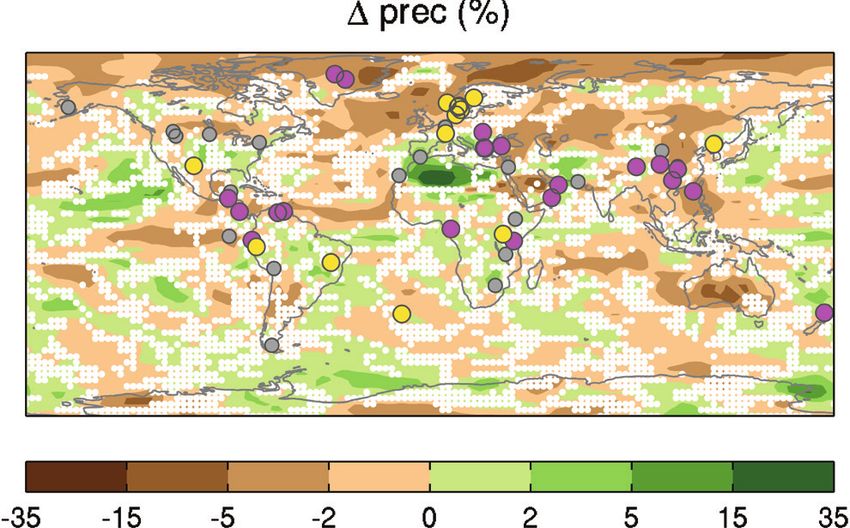
The relative contributions of these natural and anthropogenic factors change with time. FAQ 5.1, Figure 1 illustrates
those contributions based on a very simple calculation, in which the mean global surface temperature variation rep-
resents the sum of four components linearly related to solar, volcanic, and anthropogenic forcing, and to internal
5 variability. Global surface temperature has increased by approximately 0.8°C from 1870 to 2010 (FAQ 5.1, Figure
1a). However, this increase has not been uniform: at times, factors that cool the Earth’s surface—volcanic eruptions,
reduced solar activity, most anthropogenic aerosol emissions—have outweighed those factors that warm it, such
as greenhouse gases, and the variability generated within the climate system has caused further fluctuations unre-
lated to external influences.
The solar contribution to the record of global surface temperature change is dominated by the 11-year solar cycle,
which can explain global temperature fluctuations up to approximately 0.1°C between minima and maxima (FAQ
5.1, Figure 1b). A long-term increasing trend in solar activity in the early 20th century may have augmented the
warming recorded during this interval, together with internal variability, greenhouse gas increases and a hiatus
in volcanism. However, it cannot explain the observed increase since the late 1970s, and there was even a slight
decreasing trend of TSI from 1986 to 2008 (Chapters 8 and 10).
Volcanic eruptions contribute to global surface temperature change by episodically injecting aerosols into the
atmosphere, which cool the Earth’s surface (FAQ 5.1, Figure 1c). Large volcanic eruptions, such as the eruption of
Mt. Pinatubo in 1991, can cool the surface by around 0.1°C to 0.3°C for up to three years. (continued on next page)
392Information from Paleoclimate Archives Chapter 5
FAQ 5.1 (continued)
(a) Global Surface Temperature
0.8
The most important component of internal cli-
Anomaly (°C)
0.4
mate variability is the El Niño Southern Oscillation,
which has a major effect on year-to-year variations 0.0
of tropical and global mean temperature (FAQ 5.1, -0.4
Figure 1d). Relatively high annual temperatures
-0.8
have been encountered during El Niño events, such
as in 1997–1998. (b) Solar Component
0.2
The variability of observed global surface tempera-
Anomaly (°C)
tures from 1870 to 2010 (Figure 1a) reflects the com-
bined influences of natural (solar, volcanic, internal; 0.1
FAQ 5.1, Figure 1b–d) factors, superimposed on the
multi-decadal warming trend from anthropogenic
factors (FAQ 5.1, Figure 1e).
0.0
Prior to 1870, when anthropogenic emissions (c) Volcanic Component
0.0
of greenhouse gases and aerosols were smaller,
Anomaly (°C)
changes in solar and volcanic activity and internal
variability played a more important role, although
-0.1
the specific contributions of these individual fac-
tors to global surface temperatures are less certain.
Solar minima lasting several decades have often
-0.2
been associated with cold conditions. However,
these periods are often also affected by volcanic (d) Internal Variability
0.2
eruptions, making it difficult to quantify the solar
contribution.
Anomaly (°C)
At the regional scale, changes in solar activity have 0.0
been related to changes in surface climate and
atmospheric circulation in the Indo-Pacific, North-
ern Asia and North Atlantic areas. The mechanisms -0.2
that amplify the regional effects of the relatively (e) Anthropogenic Component
small fluctuations of TSI in the roughly 11-year solar
cycle involve dynamical interactions between the 0.8
Anomaly (°C)
upper and the lower atmosphere, or between the
0.6
ocean sea surface temperature and atmosphere,
0.4
and have little effect on global mean temperatures
(see Box 10.2). 0.2 5
Finally, a decrease in solar activity during the past 0.0
1880 1900 1920 1940 1960 1980 2000
solar minimum a few years ago (FAQ 5.1, Figure
Year
1b) raises the question of its future influence on
climate. Despite uncertainties in future solar activ- FAQ 5.1, Figure 1 | Global surface temperature anomalies from 1870 to 2010,
and the natural (solar, volcanic, and internal) and anthropogenic factors that
ity, there is high confidence that the effects of solar
influence them. (a) Global surface temperature record (1870–2010) relative to
activity within the range of grand solar maxima and the average global surface temperature for 1961–1990 (black line). A model
minima will be much smaller than the changes due of global surface temperature change (a: red line) produced using the sum of
to anthropogenic effects. the impacts on temperature of natural (b, c, d) and anthropogenic factors (e).
(b) Estimated temperature response to solar forcing. (c) Estimated temperature
response to volcanic eruptions. (d) Estimated temperature variability due to
internal variability, here related to the El Niño-Southern Oscillation. (e) Esti-
mated temperature response to anthropogenic forcing, consisting of a warm-
ing component from greenhouse gases, and a cooling component from most
aerosols.
393Chapter 5 Information from Paleoclimate Archives
5.2.2.2 Atmospheric Carbon Dioxide Concentrations from and did not exceed ~450 ppm during the Pliocene, with interglacial
Geological Proxy Data values in the upper part of that range between 350 and 450 ppm.
Geological proxies provide indirect information on atmospheric CO2 5.2.2.3 Past Changes in Mineral Dust Aerosol Concentrations
concentrations for time intervals older than those covered by ice
core records (see Section 5.2.2.1). Since AR4, the four primary proxy Past changes in mineral dust aerosol (MDA) are important for estimates
CO2 methods have undergone further development (Table 5.A.2). A of climate sensitivity (see Section 5.3.3) and for its supply of nutrients,
reassessment of biological respiration and carbonate formation has especially iron to the Southern Ocean (see Section 6.2). MDA concen-
reduced CO2 reconstructions based on fossil soils by approximately tration is controlled by variations in dust sources, and by changes in
50% (Breecker et al., 2010). Bayesian statistical techniques for calibrat- atmospheric circulation patterns acting on its transport and lifetime.
ing leaf stomatal density reconstructions produce consistently higher
CO2 estimates than previously assessed (Beerling et al., 2009), result- Since AR4, new records of past MDA flux have been obtained from
ing in more convergence between estimates from these two terrestrial deep-sea sediment and ice cores. A 4 million-year MDA-flux recon-
proxies. Recent CO2 reconstructions using the boron isotope proxy pro- struction from the Southern Ocean (Figure 5.2) implies reduced dust
vide an improved understanding of foraminifer species effects and evo- generation and transport during the Pliocene compared to Holo-
lution of seawater alkalinity (Hönisch and Hemming, 2005) and sea- cene levels, followed by a significant rise around 2.7 Ma when NH
water boron isotopic composition (Foster et al., 2012). Quantification ice volume increased (Martinez-Garcia et al., 2011). Central Antarc-
of the phytoplankton cell-size effects on carbon isotope fractionation tic ice core records show that local MDA deposition fluxes are ~20
has also improved the consistency of the alkenone method (Henderiks times higher during glacial compared to interglacial periods (Fischer
and Pagani, 2007). These proxies have also been applied more widely et al., 2007; Lambert et al., 2008; Petit and Delmonte, 2009). This is
and at higher temporal resolution to a range of geological archives, due to enhanced dust production in southern South America and per-
resulting in an increased number of atmospheric CO2 estimates since haps Australia (Gaiero, 2007; De Deckker et al., 2010; Gabrielli et al.,
65 Ma (Beerling and Royer, 2011). Although there is improved consen- 2010; Martinez-Garcia et al., 2011; Wegner et al., 2012). The impact of
sus between the proxy CO2 estimates, especially the marine proxy esti- changes in MDA lifetime (Petit and Delmonte, 2009) on dust fluxes in
mates, a significant degree of variation among the different techniques Antarctica remains uncertain (Fischer et al., 2007; Wolff et al., 2010).
remains. All four techniques have been included in the assessment, as Equatorial Pacific glacial–interglacial MDA fluxes co-vary with Antarc-
there is insufficient knowledge to discriminate between different proxy tic records, but with a glacial–interglacial ratio in the range of approx-
estimates on the basis of confidence (assessed in Table 5.A.2). imately three to four (Winckler et al., 2008), attributed to enhanced
dust production from Asian and northern South American sources in
In the time interval between 65 and 23 Ma, all proxy estimates of CO2 glacial times (Maher et al., 2010). The dominant dust source regions
concentration span a range of 300 ppm to 1500 ppm (Figure 5.2). An (e.g., North Africa, Arabia and Central Asia) show complex patterns
independent constraint on Early Eocene atmospheric CO2 concentra- of variability (Roberts et al., 2011). A glacial increase of MDA source
tion is provided by the occurrence of the sodium carbonate mineral strength by a factor of 3 to 4 requires low vegetation cover, seasonal
nahcolite, in about 50 Ma lake sediments, which precipitates in asso- aridity, and high wind speeds (Fischer et al., 2007; McGee et al., 2010).
ciation with halite at the sediment–water interface only at CO2 levels In Greenland ice cores, MDA ice concentrations are higher by a factor
>1125 ppm (Lowenstein and Demicco, 2006), and thus provides a of 100 and deposition fluxes by a factor 20 during glacial periods
potential lower bound for atmospheric concentration (medium confi- (Ruth et al., 2007). This is due mainly to changes in the dust sources
dence) during the warmest period of the last 65 Ma, the Early Eocene for Greenland (Asian desert areas), increased gustiness (McGee et al.,
Climatic Optimum (EECO; 52 to 50 Ma; Table 5.1), which is inconsist- 2010) and atmospheric lifetime and transport of MDA (Fischer et al.,
5 ent with lower estimates from stomata and paleosoils. Although the 2007). A strong coherence is observed between dust in Greenland ice
reconstructions indicate a general decrease in CO2 concentrations cores and aeolian deposition in European loess formations (Antoine et
since about 50 Ma (Figure 5.2), the large scatter of proxy data pre- al., 2009).
cludes a robust assessment of the second-order variation around this
overall trend. Global data synthesis shows two to four times more dust deposition
at the Last Glacial Maximum (LGM; Table 5.1) than today (Derbyshire,
Since 23 Ma, CO2 proxy estimates are at pre-industrial levels with 2003; Maher et al., 2010). Based on data–model comparisons, esti-
exception of the Middle Miocene climatic optimum (17 to 15 Ma) mates of global mean LGM dust RF vary from –3 W m–2 to +0.1 W m–2,
and the Pliocene (5.3 to 2.6 Ma), which have higher concentrations. due to uncertainties in radiative properties. The best estimate value
Although new CO2 reconstructions for the Pliocene based on marine remains at –1 W m–2 as in AR4 (Claquin et al., 2003; Mahowald et
proxies have produced consistent estimates mostly in the range 350 al., 2006, 2011; Patadia et al., 2009; Takemura et al., 2009; Yue et al.,
ppm to 450 ppm (Pagani et al., 2010; Seki et al., 2010; Bartoli et al., 2010). Models may underestimate the MDA RF at high latitudes (Lam-
2011), the uncertainties associated with these marine estimates remain bert et al., 2013).
difficult to quantify. Several boron-derived data sets agree within error
(±25 ppm) with the ice core records (Foster, 2008; Hönisch et al., 2009),
but alkenone data for the ice core period are outside the error limits
(Figure 5.2). We conclude that there is medium confidence that CO2
levels were above pre-industrial interglacial concentration (~280 ppm)
394Information from Paleoclimate Archives Chapter 5
MPWP
Dust accumulation
Southern Ocean
(g m−2 yr−1)
1
2
5
10
0 20
sea level (m)
Global
Tropical sea−surface
temperature (°C)
−100
28
26
500
24
Atmospheric CO2
400
(ppm)
300
200
100
3 2 1 0
Age (Ma)
2000
1000
Atmospheric CO2
(ppm)
500
200
CO2 proxies
Phytoplankton Boron
Stomata Liverworts
Nahcolite Paleosols
100
5
60 50 40 30 20 10 0
Age (Ma)
Figure 5.2 | (Top) Orbital-scale Earth system responses to radiative forcings and perturbations from 3.5 Ma to present. Reconstructed dust mass accumulation rate is from the
Atlantic sector of the Southern Ocean (red) (Martinez-Garcia et al., 2011). Sea level curve (blue) is the stacked d18O proxy for ice volume and ocean temperature (Lisiecki and Raymo,
2005) calibrated to global average eustatic sea level (Naish and Wilson, 2009; Miller et al., 2012a). Also shown are global eustatic sea level reconstructions for the last 500 kyr
based on sea level calibration of the d18O curve using dated coral shorelines (green line; Waelbroeck et al., 2002) and the Red Sea isotopic reconstruction (red line; Rohling et al.,
2009). Weighted mean estimates (2 standard deviation uncertainty) for far-field reconstructions of eustatic peaks are shown for mid-Pliocene interglacials (red dots; Miller et al.,
2012a). The dashed horizontal line represents present-day sea level. Tropical sea surface temperature (black line) based on a stack of four alkenone-based sea surface temperature
reconstructions (Herbert et al., 2010). Atmospheric carbon dioxide (CO2) measured from Antarctic ice cores (green line, Petit et al., 1999; Siegenthaler et al., 2005; Lüthi et al., 2008),
and estimates of CO2 from boron isotopes (d11B) in foraminifera in marine sediments (blue triangles; Hönisch et al., 2009; Seki et al., 2010; Bartoli et al., 2011), and phytoplankton
alkenone-derived carbon isotope proxies (red diamonds; Pagani et al., 2010; Seki et al., 2010), plotted with 2 standard deviation uncertainty. Present (2012) and pre-industrial CO2
concentrations are indicated with long-dashed and short-dashed grey lines, respectively. (Bottom) Concentration of atmospheric CO2 for the last 65 Ma is reconstructed from marine
and terrestrial proxies (Cerling, 1992; Freeman and Hayes, 1992; Koch et al., 1992; Stott, 1992; van der Burgh et al., 1993; Sinha and Stott, 1994; Kürschner, 1996; McElwain, 1998;
Ekart et al., 1999; Pagani et al., 1999a, 1999b, 2005a, 2005b, 2010, 2011; Kürschner et al., 2001, 2008; Royer et al., 2001a, 2001b; Beerling et al., 2002, 2009; Beerling and Royer,
2002; Nordt et al., 2002; Greenwood et al., 2003; Royer, 2003; Lowenstein and Demicco, 2006; Fletcher et al., 2008; Pearson et al., 2009; Retallack, 2009b, 2009a; Tripati et al.,
2009;Seki et al., 2010; Smith et al., 2010; Bartoli et al., 2011; Doria et al., 2011; Foster et al., 2012). Individual proxy methods are colour-coded (see also Table A5.1). The light blue
shading is a 1-standard deviation uncertainty band constructed using block bootstrap resampling (Mudelsee et al., 2012) for a kernel regression through all the data points with a
bandwidth of 8 Myr prior to 30 Ma, and 1 Myr from 30 Ma to present. Most of the data points for CO2 proxies are based on duplicate and multiple analyses. The red box labelled
MPWP represents the mid-Pliocene Warm Period (3.3 to 3.0 Ma; Table 5.1).
395You can also read