Latent Linear Adjustment Autoencoder v1.0: a novel method for estimating and emulating dynamic precipitation at high resolution - GMD
←
→
Page content transcription
If your browser does not render page correctly, please read the page content below
Geosci. Model Dev., 14, 4977–4999, 2021
https://doi.org/10.5194/gmd-14-4977-2021
© Author(s) 2021. This work is distributed under
the Creative Commons Attribution 4.0 License.

Latent Linear Adjustment Autoencoder v1.0: a novel method for
estimating and emulating dynamic precipitation at high resolution
Christina Heinze-Deml1 , Sebastian Sippel1,2 , Angeline G. Pendergrass3,4,2 , Flavio Lehner3,4,2 , and
Nicolai Meinshausen1
1 Seminar for Statistics, ETH Zurich, Zurich, Switzerland
2 Institute
          for Atmospheric and Climate Science, ETH Zurich, Zurich, Switzerland
3 Department of Earth and Atmospheric Sciences, Cornell University, Ithaca, NY, USA
4 Climate and Global Dynamics Laboratory, National Center for Atmospheric Research, Boulder, CO, USA

Correspondence: Christina Heinze-Deml (heinzedeml@stat.math.ethz.ch)

Received: 14 August 2020 – Discussion started: 28 October 2020
Revised: 27 May 2021 – Accepted: 7 July 2021 – Published: 12 August 2021

Abstract. A key challenge in climate science is to quan-          ble of the Canadian Regional Climate Model at 12 km res-
tify the forced response in impact-relevant variables such        olution over Europe, capturing, for instance, key orographic
as precipitation against the background of internal variabil-     features and geographical gradients. Using the Latent Lin-
ity, both in models and observations. Dynamical adjustment        ear Adjustment Autoencoder to remove the dynamic compo-
techniques aim to remove unforced variability from a tar-         nent of precipitation variability, forced thermodynamic com-
get variable by identifying patterns associated with circu-       ponents are expected to remain in the residual, which enables
lation, thus effectively acting as a filter for dynamically in-   the uncovering of forced precipitation patterns of change
duced variability. The forced contributions are interpreted       from just a few ensemble members. We extend this to quan-
as the variation that is unexplained by circulation. How-         tify the forced pattern of change conditional on specific cir-
ever, dynamical adjustment of precipitation at local scales       culation regimes. Future applications could include, for in-
remains challenging because of large natural variability and      stance, weather generators emulating climate model simu-
the complex, nonlinear relationship between precipitation         lations of regional precipitation, detection and attribution at
and circulation particularly in heterogeneous terrain. Build-     subcontinental scales, or statistical downscaling and trans-
ing on variational autoencoders, we introduce a novel sta-        fer learning between models and observations to exploit the
tistical model – the Latent Linear Adjustment Autoencoder         typically much larger sample size in models compared to ob-
(LLAAE) – that enables estimation of the contribution of a        servations.
coarse-scale atmospheric circulation proxy to daily precipi-
tation at high resolution and in a spatially coherent manner.
To predict circulation-induced precipitation, the Latent Lin-
ear Adjustment Autoencoder combines a linear component,           1   Introduction
which models the relationship between circulation and the
latent space of an autoencoder, with the autoencoder’s non-       Precipitation is a key climate variable that is highly relevant
linear decoder. The combination is achieved by imposing an        for impacts such as floods or meteorological drought. Precip-
additional penalty in the cost function that encourages lin-      itation simulations at high resolution (e.g. Prein et al., 2017)
earity between the circulation field and the autoencoder’s la-    are required for adaptation planning for local and regional
tent space, hence leveraging robustness advantages of linear      precipitation change in a warming climate. However, precip-
models as well as the flexibility of deep neural networks. We     itation shows large natural variability (Deser et al., 2012),
show that our model predicts realistic daily winter precipita-    and its relationship with atmospheric circulation is complex
tion fields at high resolution based on a 50-member ensem-        and nonlinear, in particular at local to regional scales and
                                                                  in heterogeneous terrain (e.g. Zorita et al., 1995). Moreover,

Published by Copernicus Publications on behalf of the European Geosciences Union.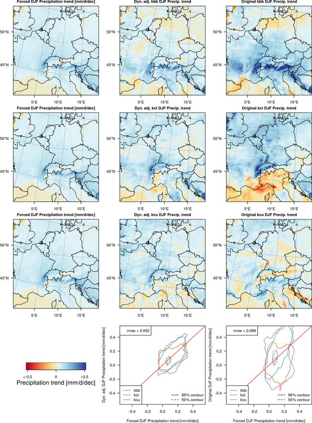
4978                                                          C. Heinze-Deml et al.: Latent Linear Adjustment Autoencoder

projected changes in precipitation are unevenly distributed        (Kingma and Welling, 2014; Rezende et al., 2014) started
across the distribution of precipitation intensity (Allen and      a whole subfield in deep learning research. Among other
Ingram, 2002; Held and Soden, 2006; Pendergrass, 2018).            things, the popularity of VAEs is due to their ability to gen-
Scaling rates depend on the return period, region, tem-            erate new images, in addition to being a powerful nonlin-
perature and moisture availability (Prein et al., 2017), and       ear dimensionality reduction technique. Our proposed Latent
changes in circulation during precipitation events (Shepherd,      Linear Adjustment Autoencoder extends the standard VAE
2014; Fereday et al., 2018). Hence, it is a key challenge to       model appropriately to enable the climate applications of in-
identify, understand, and interpret patterns of forced precipi-    terest.
tation change in model simulations and observations.                  Specifically, during training, the Latent Linear Adjustment
   Dynamical adjustment techniques have been developed to          Autoencoder encodes daily precipitation fields into a low-
separate forced and internal variability via a co-interpretation   dimensional latent space and subsequently decodes them for
of target variables such as temperature or precipitation us-       reconstruction. In addition, we formulate the objective func-
ing circulation information: a circulation proxy (such as a        tion such that the latent space can be regressed linearly on
sea-level pressure pattern) is used to estimate the circulation-   the circulation proxy. For dynamical adjustment, we use the
induced (dynamic) contribution to temperature or precipita-        estimate of the latent space based on circulation, which is
tion variability. For example, dynamical adjustment of pre-        then decoded for predicting daily precipitation fields at high
cipitation has revealed that the spatial pattern and amplitude     spatial resolution. In other words, the final model is nonlin-
of observed residual (predominant thermodynamic) precipi-          ear, consisting of a linear part and a nonlinear part, where
tation trends at the scale of the entire Northern Hemisphere       the latter is a deep neural network. It enables prediction of
mid- and high-latitude land areas are in good agreement with       the portion of the precipitation field that can be explained
the expected anthropogenically forced trends from model            by circulation (i.e. the dynamic component of precipitation).
simulations (Guo et al., 2019). Similarly, in Europe, Fere-        Moreover, several further climate science applications of the
day et al. (2018) showed that thermodynamic forced changes         Latent Linear Adjustment Autoencoder are conceivable, such
in future winter precipitation are in relatively good agree-       as for example weather generators emulating regional cli-
ment among models, while large uncertainties remain in sim-        mate model simulations, detection and attribution at subcon-
ulated forced circulation changes that may affect precipita-       tinental scales, or statistical downscaling, and are discussed
tion. While internal and forced components of precipitation        further below.
variability and change can be decomposed in large ensem-              In summary, the objectives of this paper are the following:
bles of model simulations (Deser et al., 2012; von Trentini
et al., 2019; Leduc et al., 2019), high-resolution large en-           1. We introduce a novel statistical model – the Latent Lin-
sembles are prohibitively expensive. It would be beneficial               ear Adjustment Autoencoder – as a versatile technique
to be able to estimate and identify forced precipitation pat-             for applications in climate science, particularly for mak-
terns from only a few ensemble members at impact-relevant                 ing better use of high-resolution climate simulations by
regional spatial scales.                                                  estimating circulation-induced (dynamic) precipitation
   Techniques for dynamical adjustment have relied largely                at high resolution from coarse-scale circulation infor-
on linear regression (Wallace et al., 1995, 2012; Smoliak                 mation.
et al., 2015; Sippel et al., 2019) or circulation analogue tech-
                                                                       2. We illustrate the Latent Linear Adjustment Autoencoder
niques (Yiou et al., 2007; Deser et al., 2016). Because the
                                                                          by applying it to dynamical adjustment of daily high-
fraction of variability that can be explained by these tech-
                                                                          resolution precipitation from simulations over central
niques is limited, dynamical adjustment has so far been ap-
                                                                          Europe. More specifically, the LLAAE will be used to
plied on large spatial and temporal scales (e.g. Guo et al.,
                                                                          separate forced precipitation trends from internal vari-
2019), and has also been more successful for temperature
                                                                          ability.
trends than for precipitation. Applying it to precipitation on
local or regional scales at high resolution remains a chal-
lenge.                                                             2    Dynamical adjustment using statistical learning
   In this work, we leverage recent advances in machine
learning to propose a novel statistical model – the Latent         Following Smoliak et al. (2015) and Sippel et al. (2019), we
Linear Adjustment Autoencoder (LLAAE) – suitable for dy-           frame dynamical adjustment as a statistical learning problem.
namical adjustment (and potentially further applications) in       Let Y ∈ Rh×w be the climate variable of interest on a spatial
daily, high-resolution precipitation fields. In recent years,      field of size h × w and let X ∈ Rp be input features. In the
deep learning techniques have gained in popularity in ma-          following, we consider daily precipitation fields for Y and
chine learning due to large improvements in neural network         empirical orthogonal function (EOF) time series of sea-level
architectures, optimization algorithms as well as computing        pressure (SLP) for X as a proxy for circulation. The EOF
power and frameworks. Among the class of deep generative           time series are detrended (as described below) and scaled to
models, the introduction of variational autoencoders (VAEs)        unit variance; in the EOF computation, we do not weight

Geosci. Model Dev., 14, 4977–4999, 2021                                              https://doi.org/10.5194/gmd-14-4977-2021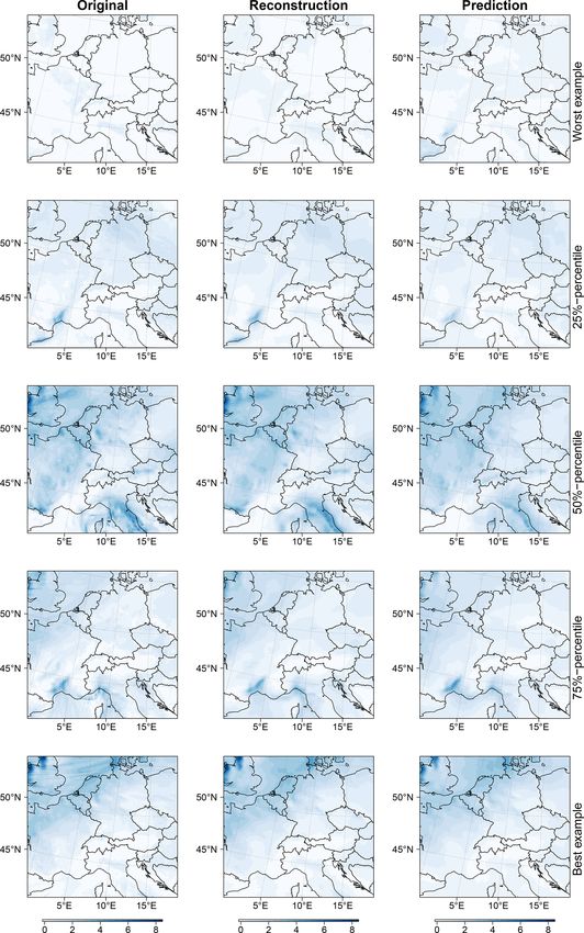
C. Heinze-Deml et al.: Latent Linear Adjustment Autoencoder                                                                  4979

by area. A variety of climate variables instead of precipita-        We extend the standard VAE model to make it suitable
tion could be taken as Y ; results for daily temperature can be   for dynamical adjustment by adding a linear component h
found in Appendix C.                                              to the architecture. The linear component h takes X as in-
   Let X be the n × p matrix, where each column contains          put features and predicts the latent space variables L of the
one input feature with n data points. Each data point is in       VAE; thus, we call the overall model the “Latent Linear Ad-
our case a simulation from a regional climate model (RCM),        justment Autoencoder”. Using an appropriate training objec-
and each column corresponds to one of p EOF components            tive (see Eq. 3), we enforce that when linearly predicting
of SLP, from the RCM but at coarsened resolution. Let Y be        the latent space variables L with X, L̂ = h(X), the resulting
the n×h×w tensor that represents the precipitation intensity      decoded prediction ŶX = d(L̂) = d(h(X)) to be close to Y .
for each data point in a spatial field. Below, we present our     The motivation behind this loss function is that the combined
proposed statistical model, which estimates the circulation-      model, which consists of the combination of h and d, should
induced component of precipitation ŶX :                          explain as much variance in Y as possible, while using only
                                                                  the input X. In other words, it should capture the circulation-
ŶX = f (X),                                               (1)    induced signal in Y . The advantage of combining the linear
                                                                  model h with the nonlinear decoder of the VAE d is that the
where f is a generic nonlinear function. Let R̂ denote the        overall model is very expressive, while the estimation of h
residuals R̂ = Y − ŶX that remain. Since ŶX is the precip-      remains relatively simple.
itation explained primarily by variations in circulation, R̂ is      In more detail, we consider the following objective to
the precipitation primarily unexplained by circulation. If SLP    train the encoder e and decoder d with associated parame-
is unaffected by external forcing, then this residual contains    ters θ = (θe , θd ) of our proposed Latent Linear Adjustment
the signal induced by the thermodynamic component of the          Autoencoder:
external forcing, since the variability due to circulation has
                                                                  Lθ = LVAE + λLL .                                            (2)
been removed. If instead external forcing does affect SLP,
then the dependence between X and Y that arises due to the        LVAE is the standard VAE objective for real-valued input
common influence of the external forcing would bias the es-       data, consisting of a reconstruction loss and the Kullback–
timation of f . To avoid potential forced trends in SLP pro-      Leibler divergence between the distribution of the encoded
jecting onto the thermodynamic component of the external          inputs and the prior distribution of the latent space, here cho-
forcing in Y , we detrend the daily SLP EOF time series as        sen to be a standard multivariate Gaussian distribution (for
follows. We ensure that they are orthogonal to the smoothed,      details, see Kingma and Welling, 2014; Rezende et al., 2014).
first EOF of the January ensemble mean by regressing the          LL is the extension to the objective that we propose:
time series against the ensemble mean and using the corre-
sponding residuals as input features X. The reasoning behind      LL =k Y − ŶX k22 =k Y − d(h(X))k22 ,                        (3)
this step is that a forced trend in SLP will be approximately
                                                                  and λ is a tuning parameter that steers the relative importance
captured in the first EOF of the SLP ensemble mean. Here,
                                                                  of the two loss functions in the overall objective (Eq. 2). The
we use the January ensemble mean as a proxy for December–
                                                                  autoencoder and the linear model are trained iteratively in an
February SLP. For simplicity, we refer to the detrended and
                                                                  alternating fashion. In the first step, the objective Lθ is opti-
scaled SLP EOF time series simply as the “SLP time series”
                                                                  mized while h is treated as fixed. In a second step, the linear
in the following.
                                                                  component h of the Latent Linear Adjustment Autoencoder
2.1   Latent Linear Adjustment Autoencoder: proposed              is trained with squared error loss, treating the encoder and
      deep autoencoder model for dynamical adjustment             decoder parameters as fixed:
                                                                             Lk22 =k e(Y) − h(X)k22 .
                                                                  Lθh =k L − b                                                 (4)
We build on variational autoencoders (Kingma and Welling,
2014; Rezende et al., 2014), which can be understood as a         The parameters of the encoder and decoder (θe , θd ) and those
(typically nonlinear) dimensionality reduction method. An         of the linear model h, θh , are coupled, since the linear model
autoencoder consists of an “encoder” e that maps Y to the         aims to predict the latent space variables L, which are subject
low-dimensional latent space L ∈ Rl , L = e(Y ), and a “de-       to change during the training of the encoder and the decoder.
coder” d which in turn maps L to the reconstruction of Y ,        At the same time, the autoencoder should be trained such
Ŷ = d(L) = d(e(Y )). This scheme is illustrated in Fig. 1,       that a linear regression from L on X achieves a small error in
which depicts the reconstruction of precipitation fields. The     Eq. (3), which is accomplished with this procedure for train-
VAE objective encourages the distribution of the latent space     ing the components. In practice, we train the model using the
variables L to be close to a chosen prior distribution, typi-     Adam optimizer (Kingma and Ba, 2015). All details related
cally a standard multivariate Gaussian distribution, and also     to training the model, such as architecture and hyperparam-
ensures that Ŷ ≈ Y . The encoder and the decoder are param-      eter choices, as well as code to reproduce our experimental
eterized as (deep) neural networks.                               results, can be found in Appendix A.

https://doi.org/10.5194/gmd-14-4977-2021                                            Geosci. Model Dev., 14, 4977–4999, 2021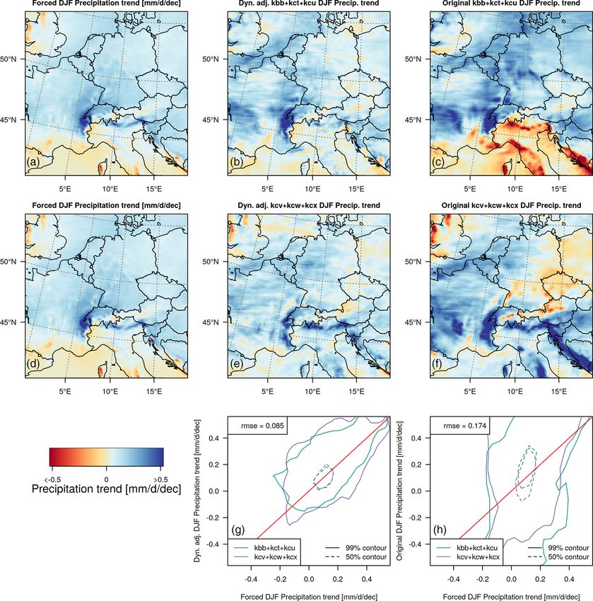
4980                                                                C. Heinze-Deml et al.: Latent Linear Adjustment Autoencoder

Figure 1. Illustration of a standard autoencoder model: the spatial fields Y are fed to the encoder e which maps them to the latent space
variables L (illustrated in blue). These are in turn fed to the decoder d which computes a reconstruction of the input, Ŷ .

                                                                         a function of coarse-scale circulation may enable several ad-
                                                                         ditional climate science applications, which are briefly dis-
                                                                         cussed in Sect. 4.

                                                                         3     Data and evaluation

                                                                         3.1    Data

                                                                         To evaluate our statistical model, we use the Canadian Re-
                                                                         gional Climate Model Large Ensemble (CRCM5-LE, Leduc
                                                                         et al., 2019) which is based on a dynamically down-
                                                                         scaled version of the 50-member CanESM2 large ensem-
                                                                         ble (CanESM2-LE). CanESM2-LE is an initial-condition en-
                                                                         semble of climate change projections (Kirchmeier-Young
                                                                         et al., 2017) run with the Canadian Earth System Model
                                                                         (Arora et al., 2011), globally on a spatial resolution of 2.8◦ .
                                                                         CanESM2-LE combines so-called “macro” and “micro” ini-
                                                                         tializations: to achieve different 1950 ocean states (the macro
                                                                         initialization), five historical spinup runs are branched from
                                                                         a long pre-industrial (1850) control run to which small ran-
                                                                         dom atmospheric perturbations and then time-varying forc-
Figure 2. Illustration of the Latent Linear Adjustment Autoencoder       ings are applied until 1950. Then, for the micro ensemble
after training: the input features X (illustrated in grey) are fed to    (where members have the same initial conditions in the ocean
the linear model h which yields a prediction for the latent space        but differ in their atmosphere), a second set of random pertur-
variables L (illustrated in light blue). These are in turn fed to the    bations is applied in 1950 to generate 10 runs spanning 1950–
decoder which computes a prediction of the spatial field based on        2006 for each of the five historical spinups, with a time-
X only, ŶX . Training the models e, d, and h is performed iteratively   varying historical forcing scenario applied through 2006. The
in an alternating fashion.                                               runs continue from 2006 until 2100 with RCP8.5 forcing
                                                                         (Kirchmeier-Young et al., 2017).
                                                                            This approach yields 50 approximately independent real-
   After training the components e, d, and h, we no longer               izations of the climate system (Leduc et al., 2019). Each of
need the encoder to perform dynamical adjustment on un-                  the global simulations has been downscaled using the Cana-
seen test data. This is illustrated in Fig. 2. We predict the            dian Regional Climate model version 5 (Martynov et al.,
latent space variables with the linear model h using the SLP             2013) to a resolution of approximately 0.11◦ (≈ 12 km) over
time series as input X. The resulting predictions are fed to the         Europe for the 1950–2099 period, which yields the regional
decoder, which outputs predictions of the spatial field based            large ensemble CRCM5-LE. More details about the mod-
only on X. In other words, we obtain the spatial field of pre-           elling setup and evaluation of the simulations are available
cipitation which can be explained by circulation.                        in Leduc et al. (2019).
   The spatial field is modelled jointly in our approach –
the optimization is performed over the whole spatial field
at once – in contrast to Sippel et al. (2019), where a sepa-
rate model needed to be trained for each grid cell. The joint
modelling of the daily high-resolution precipitation field as

Geosci. Model Dev., 14, 4977–4999, 2021                                                  https://doi.org/10.5194/gmd-14-4977-2021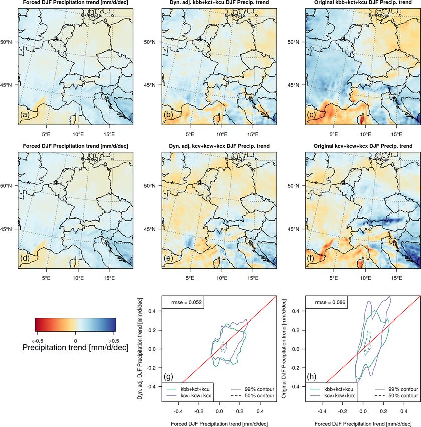
C. Heinze-Deml et al.: Latent Linear Adjustment Autoencoder 4981
3.2 Experimental setup atively poorly to cases where the LLAAE performs well (in
terms of R 2 ). To highlight the precipitation features, these
3.2.1 Target variables examples are displayed after the data have been square-root
transformed. We compute the grid-cell-wise mean squared
We focus on precipitation as the target climate variable error (MSE) of predictions ŶX and the proportion of ex-
throughout the main text. A subset of results for tempera- plained variance (R 2 ) based on the daily data from the hold-
ture can be found in Appendix C. For the precipitation fields, out ensemble member “kbb”. The results for the other hold-
we apply a square-root transformation to stabilize the autoen- out ensemble members are very similar. We further evaluate
coder training; the results presented in Sect. 4 are based on the predictions within a dynamical adjustment framework de-
transforming the results back to the original scale (mm d−1 ), scribed in the next paragraph.
except for some visualizations where indicated in the cap-
tions. The spatial fields we consider have 128 × 128 grid 3.2.5 Dynamical adjustment
cells; i.e. they are a subset of the original 280 × 280 field,
cropped around central Europe (with boundaries 42–54.8◦ N, We evaluate the extent to which the forced response of pre-
0–18.9◦ E). We aggregate the data (which are hourly) to daily cipitation can be uncovered with a small number of en-
averages. semble members using dynamical adjustment (e.g. Deser
et al., 2016). Specifically, we quantify how well the long-
3.2.2 Input features term “forced response” (i.e. the average across all 50 ensem-
ble members) can be approximated by the residuals of our
SLP is regridded to a spatial resolution of 1 × 1◦ before com- predictions (the difference between precipitation simulated
puting the EOFs as described in Sect. 2, so that the model by the RCM and the circulation-induced component of pre-
predicts high-resolution precipitation from only a coarse- cipitation predicted by the Latent Linear Adjustment Autoen-
resolution proxy of atmospheric circulation. We aggregate coder). In other words, dynamical adjustment acts as a filter
the data (3 h) to daily averages. SLP data are also taken for short-term “circulation-induced” precipitation variability.
from the original 280 × 280, 0.12◦ resolution Coordinated Recall that we expect the residuals to primarily contain the
Regional Climate Downscaling Experiment – European Do- thermodynamic component of change (Deser et al., 2016).
main (EURO-CORDEX) (WCRP, 2015) and regridded to a However, it is important to stress that the residual is not a
regular 1 × 1◦ grid that broadly covers the region of −15 to perfect proxy for thermodynamical change, because it may
35–64◦ N, 35◦ E (see Fig. 9, top). contain effects from feedbacks, remaining internal variabil-
ity, and circulation components not directly captured by SLP.
3.2.3 Time periods and training/test splits Moreover, since the SLP data are detrended prior to the ap-
plication of the method, long-term dynamical changes may
We use RCM simulation data from 1955 to 2100 to allow for
even be part of the residuals. In addition to analysing the
5 years of spinup. We train our model using daily data from
forced response in seasonal precipitation totals, we evaluate
December to February (DJF) from nine ensemble members
the estimation of the forced precipitation response for two
(“kba”, “kbc”, “kbe”, “kbg”, “kbi”, “kbk”, “kbm”, “kbq”,
composites of atmospheric circulation based on EOF analy-
“kbs”). The results in the main text are based on training
sis of SLP.
data that comprise the years 1955–2070. In Appendix B, we
present results based on the shorter training time period from
1955 to 2020, using the same ensemble members. This cor- 4 Results and discussion
responds to a reduction in the amount of training data points
of approximately 43 % and serves as a sensitivity test to 4.1 Reconstructed and predicted spatial fields
the amount of training data. Furthermore, we evaluate our
trained models on the remaining 41 ensemble members that We begin by showing a selection of reconstructed precipita-
were left out of training. We refer to these as “holdout en- tion fields Ŷ from the holdout ensemble member “kbb” (cen-
semble members”. tre, Fig. 3), which illustrates the skill of the encoder and de-
coder, and predictions ŶX (right, Fig. 3), which illustrate the
3.2.4 Evaluation of predictions skill of the linear latent model h against the original RCM-
simulated precipitation Y (left, Fig. 3). The reconstruction
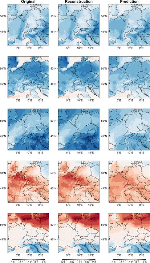
To illustrate the spatial coherence of our approach, we show quality, i.e. the similarity between the left and the centre col-
five example target (daily) data points of Y , their reconstruc- umn, is quite high, though not all fine details are reproduced
tions Ŷ , and the predictions ŶX from the holdout ensemble (which is to be expected). The predictions ŶX (right column)
member “kbb” (Fig. 3). These examples are chosen for dif- are computed using the linear model h and the decoder d
ferent percentiles of the distribution of the R 2 values (i.e. with SLP time series as inputs. For the worst example (in
proportion of explained variance). As such, they show the terms of R 2 ; first row), the original spatial field shows that
range between data points where the LLAAE performs rel- this corresponds to a day with very low precipitation, while
https://doi.org/10.5194/gmd-14-4977-2021 Geosci. Model Dev., 14, 4977–4999, 2021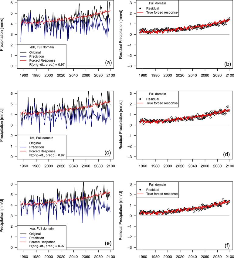
4982                                                                C. Heinze-Deml et al.: Latent Linear Adjustment Autoencoder

Figure 3. Examples of (i) original precipitation fields (left column), (ii) reconstructions (centre column), and (iii) predictions (right column).
The examples are chosen such that the R 2 value of the prediction increases from top to bottom: the first row shows the worst example in
the holdout dataset, the last row shows the best example, and the remaining rows show       √ examples at the 25th, 50th, and 75th percentiles,
respectively. For better visibility, data are square-root transformed. Hence, the units are mm d−1 .

Geosci. Model Dev., 14, 4977–4999, 2021                                                       https://doi.org/10.5194/gmd-14-4977-2021
C. Heinze-Deml et al.: Latent Linear Adjustment Autoencoder 4983
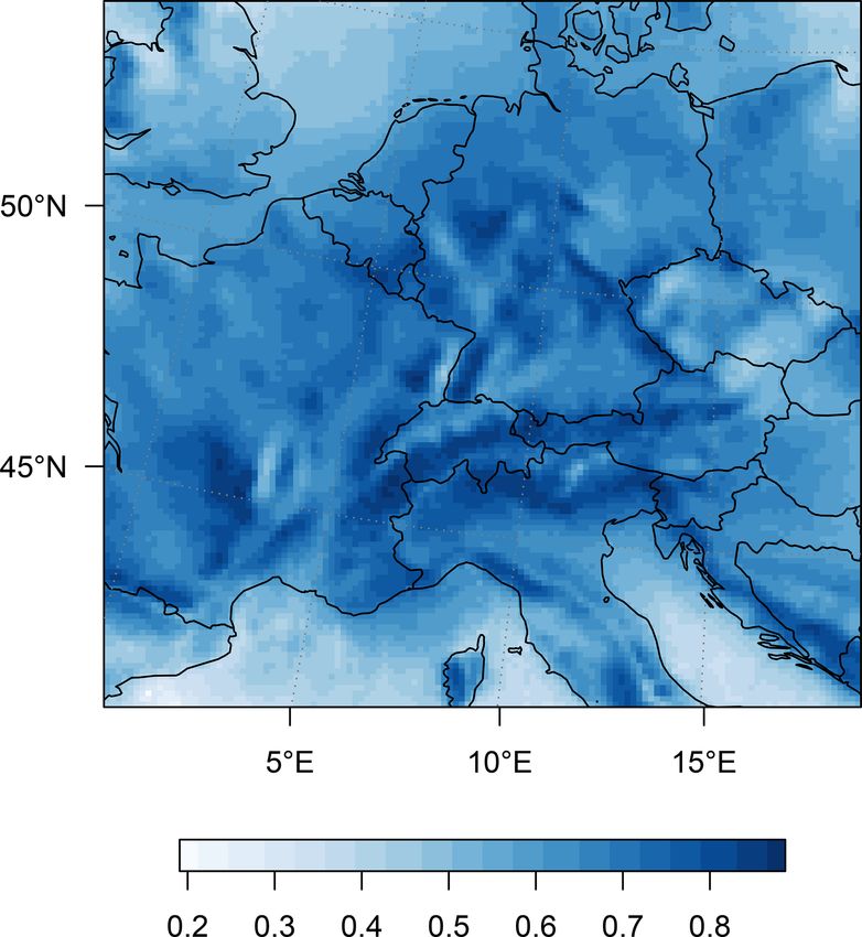
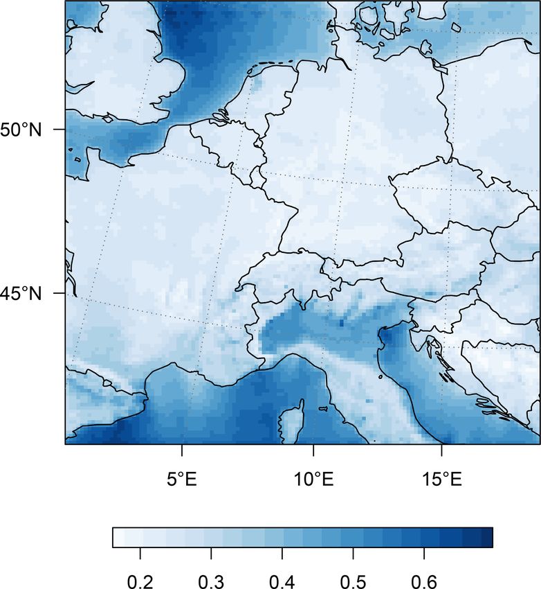
Figure 4. MSE (based on precipitation data in mm d−1 ) for each Figure 5. Proportion of variance explained (R 2 ) for each grid cell
grid cell for the precipitation predictions. for the precipitation predictions.
the LLAAE predicts larger precipitation in some regions (e.g.
south of France), resulting in a very low R 2 value. For the 4.2 Extraction of forced precipitation trends at high
other rows (25 % percentile – best example), the predictions spatial resolution
resemble the original image fairly well. For dynamical ad-
justment, we use the residuals R̂, which are computed as the In this subsection, we evaluate our predictions of the
difference between the original fields Y (left column) and the circulation-induced component in the framework of dynami-
predictions (right column). cal adjustment (Deser et al., 2016). That is, we test the extent
The proposed model yields spatially coherent predictions to which the forced response of regional high-resolution pre-
and explains a large proportion of the variance of Y . The cipitation obtained from averaging across the full 50-member
skill of precipitation predicted with the Latent Linear Ad- ensemble can be approximated by the residuals of our predic-
justment Autoencoder is quantified in Fig. 4, which shows tions from a single or from relatively few ensemble members.
the grid-cell-wise MSE over all December–February days for The thermodynamic component of the variation in precipita-
the holdout ensemble member “kbb”. The spatial pattern of tion, which is driven by temperature change and unrelated to
MSEs (Fig. 4) largely reflects the pattern of precipitation as dynamically induced variability, should remain in the resid-
simulated by the RCM. Prediction errors are high over het- uals (e.g. Deser et al., 2016). Dynamical adjustment hence
erogeneous terrain, likely linked to orographic precipitation, acts to reduce short-timescale circulation-induced variability,
in particular on the western sides of mountain ranges such thus increasing signal-to-noise ratios of the long-term, forced
as the Alps in central Europe, the Appenines in Italy, the component (Deser et al., 2016).
Dinaric Alps in southeastern Europe, and smaller ranges lo- The effect of dynamical adjustment can be seen in Fig. 6. It
cated in France and Germany. Prediction errors are also high shows time series of domain-average (land only) December–
at the west coast of the UK, whereas mean squared prediction February seasonal precipitation totals simulated by the high-
errors appear relatively low over low-altitude regions (e.g. resolution RCM, the predictions of the circulation-induced
northern France, Benelux, and north Germany). The spatial component for three holdout ensemble members, and the
pattern of R 2 (the fraction of explained variance, Fig. 5) forced response. All three RCM ensemble members show
shows a more nuanced pattern dominated by a land–sea con- an increasing trend in seasonal precipitation totals across
trast. Over land, the circulation proxy generally explains a the 21st century, over which large interannual variability is
high proportion of variance (up to ≈ 90 %), especially on the superimposed. In contrast, the predicted circulation-induced
western slopes of mountain ranges, which receive a large components capture the interannual precipitation variabil-
fraction of their precipitation from large-scale circulation- ity well, but they do not show discernible trends. Conse-
induced events. In contrast, the fraction of variance explained quently, the residuals have relatively smoothly increasing
by circulation-induced precipitation is smaller on the eastern trends, which match the magnitude of the forced precipita-
sides of mountain ranges, and particularly low over oceanic tion trend well (Fig. 6, right panels). This demonstrates suc-
regions (which we do not interpret in this study). cessful dynamical adjustment of continental-scale seasonal
precipitation totals using the Latent Linear Adjustment Au-
toencoder.
https://doi.org/10.5194/gmd-14-4977-2021 Geosci. Model Dev., 14, 4977–4999, 2021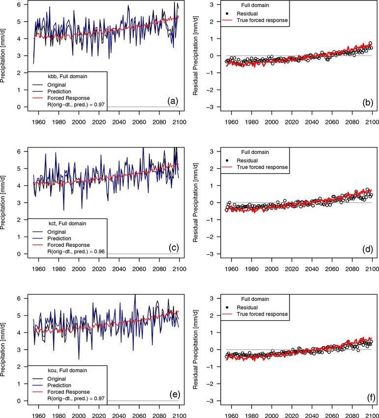
4984                                                             C. Heinze-Deml et al.: Latent Linear Adjustment Autoencoder

Figure 6. Dynamical adjustment of the full domain (land grid cells only) using autoencoders; (left) seasonal precipitation totals simulated
by three members of the high-resolution RCM in black (top: “kbb”, middle: “kct”, bottom: “kcu”), the predicted (“circulation-induced”)
component for three “holdout” ensemble members (blue), and the forced response (average across all 50 members, red); (right) residuals
from the prediction (black dots) and the forced response (red).

   It is more challenging, however, to identify and evaluate            over the Mediterranean Sea). Increases in winter precipita-
the forced precipitation response at the local scale of individ-        tion across most parts of the domain are largely due to ther-
ual grid points. To this end, Fig. 7 shows the spatial pattern          modynamic and lapse rate changes (e.g. Brogli et al., 2019).
of forced 50-year (2020–2069) precipitation trends, the pat-            Locally, forced precipitation trends are larger over heteroge-
tern of dynamically adjusted precipitation trends, and “raw”            neous terrain, which may be due to forced dynamic compo-
precipitation trends in RCM simulations for three holdout en-           nents that are independent of SLP (Shi and Durran, 2014).
semble members. The forced response of winter precipitation             The latter paper shows idealized simulations of the forced
change is dominated by a north–south contrast. The northern             response of orographic precipitation, which is dynamic, but
part of the domain is projected to experience a precipitation           it is driven by changes in vertical velocity on the upslope
increase in the 21st century, while decreases in precipitation          side that enhances orographic precipitation, which could be
are projected for the southernmost part of the domain (mainly           separate from the changes in upslope wind speed and thus

Geosci. Model Dev., 14, 4977–4999, 2021                                                  https://doi.org/10.5194/gmd-14-4977-2021
C. Heinze-Deml et al.: Latent Linear Adjustment Autoencoder                                                                             4985

Figure 7. Dynamical adjustment of 50-year winter precipitation trends (2020–2069); (left column) forced precipitation response (2020–2069
linear winter precipitation trends averaged over all 50 ensemble members); (middle column) linear 50-year winter precipitation trends in three
randomly selected dynamically adjusted ensemble members (top: “kbb”, middle: “kct”, bottom: “kcu”); (right column) linear 50-year winter
precipitation trends in the original ensemble members (top: “kbb”, middle: “kct”, bottom: “kcu”); (bottom row) scatter plot contour lines
of 50-year precipitation trends in the forced response against 50-year precipitation trends over land in dynamically adjusted (middle) and
originally simulated ensemble members (right).

https://doi.org/10.5194/gmd-14-4977-2021                                                     Geosci. Model Dev., 14, 4977–4999, 2021
4986                                                             C. Heinze-Deml et al.: Latent Linear Adjustment Autoencoder

                                                                      SLP. Vertical velocity could increase because of the increas-
                                                                      ing moisture with warming.
                                                                         However, large variability in individual ensemble mem-
                                                                      bers is superimposed on the signal of forced change (Fig. 7,
                                                                      right), consistent with the large role of internal variability
                                                                      even on multi-decadal timescales (Leduc et al., 2019). For
                                                                      example, ensemble member “kct” (second row) produces a
                                                                      relatively strong drying trend over northern Italy, which is
                                                                      entirely due to internal variability. The dynamically adjusted
                                                                      version of “kct” shows only very weak drying in northeastern
                                                                      Italy, whereas it shows an increased precipitation trend con-
                                                                      sistent with the forced response at all other locations in north-
                                                                      ern Italy. Similar differences can be seen between the ad-
                                                                      justed and unadjusted trends for the other holdout ensemble
                                                                      members. Overall, the correlation of 50-year trends at a sin-
                                                                      gle location from a single ensemble member with the trend
                                                                      in the 50-member forced response is rather low (R = 0.4,
                                                                      RMSE = 0.098). However, the dynamically adjusted single
                                                                      ensemble members are more strongly correlated with the
                                                                      forced response and capture it more accurately (R = 0.58,
                                                                      RMSE = 0.052).
                                                                         Figure 8 (top panel) shows the RMSE for the recon-
                                                                      struction of forced 50-year precipitation trends (i.e. the 50-
                                                                      member average), via dynamical adjustment and the aver-
                                                                      aging of original ensemble members, as a function of the
                                                                      number of ensemble members n. With an increasing num-
                                                                      ber of ensemble members (n), the reconstruction RMSE of
                                                                      the forced response is considerably reduced. Hence, dynami-
                                                                      cal adjustment is particularly useful when only few members
                                                                      are available, e.g. for small ensembles up to five members.
                                                                      If only one member is available, the reconstruction RMSE
                                                                      of the forced 50-year precipitation trend is reduced by more
                                                                      than half via dynamical adjustment. Conversely, to achieve
                                                                      the same RMSE of a single dynamically adjusted ensemble
                                                                      member, an ensemble average of about four to six mem-
                                                                      bers would be required (Fig. 8, top panel). On the other
                                                                      hand, for ensembles with more than about 14 members, dy-
                                                                      namical adjustment does not improve the ability to recon-
                                                                      struct the forced response. Moreover, dynamical adjustment
                                                                      reduces not only the reconstruction RMSE but also reduces
                                                                      the spread of the distribution across ensemble members, as
                                                                      indicated by the boxes and whiskers in Fig. 8 (top panel).
                                                                      The overall reduction of the reconstruction RMSE also holds
                                                                      particularly for specific circulation regimes (Fig. 8, middle
                                                                      and bottom panels) and is discussed in the next subsection.

Figure 8. RMSE of 50-year trends, calculated by averaging n mem-      4.3   Elucidating forced precipitation trends for specific
bers, compared to 50-year trends using 50-member ensemble av-               circulation composites at high spatial resolution
erage (“forced response”). RMSEs are based on land grid cells
only and shown for averaging n original ensemble members (black)      While dynamical adjustment of long-term trends of temper-
and averaging n dynamically adjusted ensemble members (red).          ature and precipitation has become a standard tool for the
Trends are calculated over the entire DJF season (a) and only for     detection of forced thermodynamic trends (Smoliak et al.,
EOF1+ (b) and EOF1- situations (c). Boxplot whiskers indicate         2015; Deser et al., 2016; Guo et al., 2019; Lehner et al.,
2.5th and 97.5th percentiles (boxes show 25th and 75th percentiles)   2018), a bigger challenge is to assess forced trends in specific
of RMSE distribution obtained from bootstrapping from the 41
                                                                      circulation regimes. One example would be summer heat
holdout ensemble members.

Geosci. Model Dev., 14, 4977–4999, 2021                                                https://doi.org/10.5194/gmd-14-4977-2021
C. Heinze-Deml et al.: Latent Linear Adjustment Autoencoder 4987 Figure 9. (a) First empirical orthogonal function of sea-level pressure over the full domain of the regional model. (b, c) Winter precipitation anomalies for the 25 % of days that show the strongest (b) and weakest (c) projection on the pattern of the first EOF (i.e. days with a strong zonal SLP gradient and hence dominant westerly flow, b, and days with weak to absent zonal SLP gradients, c). waves related to specific circulation conditions (Jézéquel bottom). Note that the principal component time series asso- et al., 2018). ciated with EOF1 does not show any discernible trend un- Thus, we assess to what extent the forced precipitation re- til the late 21st century, so we do not expect large forced sponse can be uncovered under specific circulation condi- changes in the SLP variability patterns over Europe. On win- tions from a small number of ensemble members. We cre- ter days with strong positive EOF1 (“EOF1+”, roughly anal- ate composites of the dominant mode of atmospheric winter ogous to NAO+), i.e. a pronounced north–south pressure gra- circulation over Europe as diagnosed by EOF analysis over dient, increased westerly winds bring mild and moist air from the historical period (1955–2020) in the RCM simulations. the Atlantic into central Europe (Fig. 9, bottom left). Con- The first EOF of the coarse-resolution SLP field is shown versely, the opposite regime suppresses westerlies, hence in- in Fig. 9 (top). The dominant mode has a meridional gradi- ducing drier conditions on average (Fig. 9, bottom right) ent, with low-pressure anomalies over northern Europe and which are also accompanied by colder temperatures. high-pressure anomalies over the Mediterranean. Although For the 50-year forced precipitation trend on “EOF1+” the domain includes only a small fraction of the North At- winter days (obtained by averaging across all ensemble lantic, the dipole character of the EOF spatial pattern resem- members), there is a more pronounced precipitation increase bles the North Atlantic Oscillation (NAO). on the western slopes of the Alps and in most parts of the do- We now generate composites of “EOF1+” and “EOF1- main north and west of the Alps (Fig. 10, left panel). Mean- ” regimes by isolating days that exceed the 75th percentile while, precipitation decreases in the EOF1+ regime over (“EOF1+”) and those that fall below the 25th percentile southern Europe. (“EOF1-”) in terms of the first principal component (Fig. 9, https://doi.org/10.5194/gmd-14-4977-2021 Geosci. Model Dev., 14, 4977–4999, 2021
4988                                                             C. Heinze-Deml et al.: Latent Linear Adjustment Autoencoder

Figure 10. Dynamical adjustment of 50-year winter precipitation trends (2020–2069) under the “EOF1+” regime (25 % of all days that
project strongest on the first EOF, i.e. those that show a strong westerly flow). (a, d) Linear forced winter precipitation trends under the
“EOF1+” regime (2020–2069). (b, e) Linear 50-year winter precipitation trends in an average of three randomly selected dynamically ad-
justed ensemble members. (c, f) Linear 50-year winter precipitation trends in an average of three corresponding original ensemble members.
(g, h) Scatter plots of 50-year precipitation trends in the forced response against 50-year precipitation trends over land in dynamically
adjusted (g) and originally simulated ensemble members (h).

   Raw simulations for sets of three holdout members show               particularly well captured; the pattern RMSE is reduced sub-
variable 50-year (2020–2069) precipitation trends under the             stantially (RMSE = 0.085).
“EOF1+” regime (Fig. 10, right panel), where the spatial                   Forced precipitation trends for 2020–2069 under “EOF1-”
pattern of each set of three averaged members only weakly               conditions differ from “EOF1+” conditions due to a change
resembles the forced pattern (RMSE = 0.174). The dynam-                 in the synoptic situation: the forced spatial pattern has gen-
ically adjusted holdout members reveal a pattern that more              erally weaker precipitation changes (due to overall drier
closely resembles the forced response pattern (Fig. 10, mid-            conditions during “EOF1-”), and precipitation increases are
dle panel), where forced changes in mountainous regions are             confined towards southeastern Europe (Fig. 11, left panel).

Geosci. Model Dev., 14, 4977–4999, 2021                                                   https://doi.org/10.5194/gmd-14-4977-2021
C. Heinze-Deml et al.: Latent Linear Adjustment Autoencoder                                                                               4989

Figure 11. Dynamical adjustment of 50-year winter precipitation trends (2020–2069) under the “EOF1-” regime (25 % of all days that project
weakest on the first EOF). (a, d) Linear forced winter precipitation trends under the “EOF1-” regime (2020–2069). (b, e) Linear 50-year
winter precipitation trends in an average of three randomly selected dynamically adjusted ensemble members. (c, f) Linear 50-year winter
precipitation trends in an average of three corresponding original ensemble members. (g, h) Scatter plots of 50-year precipitation trends in the
forced response against 50-year precipitation trends over land in dynamically adjusted (g) and originally simulated ensemble members (h).

Meanwhile, over large regions north and west of the Alps,                 the Latent Linear Adjustment Autoencoder may be applica-
precipitation changes only weakly under these circulation                 ble to understanding the dynamical component in extreme
conditions. Spatial patterns of dynamically adjusted ensem-               precipitation events. While the LLAAE may be able to fill
ble members (Fig. 11, middle panel) have a closer corre-                  an important gap in reconstructing the dynamical component
spondence to the forced pattern than to the spatial patterns              of daily precipitation fields, possibly including days with ex-
of “raw” 50-year trends (Fig. 11, right panel). The recon-                treme precipitation (at least, the component proportional to
struction RMSE of the forced response is again substantially              surface pressure), it exhibits a tendency to smooth predicted
reduced (RMSE = 0.052 for dynamically adjusted grid cells;                precipitation fields (Fig. 3), which would presumably result
RMSE = 0.086 for raw trends).                                             in somewhat underpredicted extreme events. However, a de-
   The application of dynamical adjustment to composites of               tailed evaluation of the LLAAE in the context of extreme
specific circulation regimes raises the question as to whether            events will be the focus of future work.

https://doi.org/10.5194/gmd-14-4977-2021                                                       Geosci. Model Dev., 14, 4977–4999, 2021
4990                                                           C. Heinze-Deml et al.: Latent Linear Adjustment Autoencoder

   Overall, we conclude that dynamical adjustment enables           stead of training the LLAAE based on simulations from nine
approximating the forced response from high-resolution sim-         ensemble members (as done in this work). Indeed, as ma-
ulations with only a few ensemble members. This is possible         chine learning algorithms are known to require rather large
for both long-term trends in seasonal precipitation totals as       amounts of training data, “proving” the case of LLAAE
well as for trends under more specific circulation regimes.         dynamical adjustment in a large ensemble may not be as
The improvement for the “EOF1+” and “EOF1-” circula-                straightforward. While we have shown that dynamical ad-
tion regimes can be evaluated from Fig. 8 (middle and bot-          justment based on LLAAEs reduces the number of ensemble
tom panels), where reconstruction RMSEs of forced 50-year           members required to identify a proxy of the forced response
precipitation trends, based on one ensemble member, are re-         for local-scale 50-year winter precipitation trends substan-
duced by up to about a factor of 2 by using dynamical adjust-       tially (Fig. 8), this approach evidently requires several en-
ment based on the Latent Linear Adjustment Autoencoder.             semble members for training. While the results shown here
To achieve a similar forced response reconstruction RMSE,           are based on training the Latent Linear Adjustment Autoen-
an ensemble average of about four to six members would be           coder with data from nine ensemble members (1955–2070
required (Fig. 8) both for seasonal trends (top panel) and the      period), we have tested that the accuracy remains virtually
trends under specific circulation composites.                       identical if trained with about 43 % less training data (nine
                                                                    ensemble members but training only on 1955–2020, Ap-
4.4    Dynamical adjustment uncertainties,                          pendix B), thus highlighting robustness of the method against
       computational costs, and future applications                 reasonable changes to the amount of training data.
                                                                       Beyond the computational aspects, however, we antici-
One of the main uncertainties in dynamical adjustment is the        pate the ultimate applications of LLAAE-based dynamical
question of whether and how to detrend the climate data (cir-       adjustment not on a large ensemble (where the forced re-
culation fields and/or precipitation) prior to dynamical ad-        sponse is typically approximated with the ensemble average,
justment. This is somewhat subjective and often discussed           Deser et al., 2020) but instead on simulations with models
as an inherent uncertainty in the literature (see, e.g. Deser       where only one or a few ensemble members may be avail-
et al., 2016; Lehner et al., 2017, 2018, for a discussion about     able such as projections with regional climate models (Ja-
trend removal). Forced changes in European winter SLP are           cob et al., 2014). Hence, the results presented in this work
highly uncertain, and models disagree on the sign and pat-          are intended as a proof-of-concept study within a large en-
terns of forced circulation change (Fereday et al., 2018),          semble. As the next step, we envision the application to dif-
while thermodynamic aspects are typically considered more           ferent climate models (e.g. training on a large ensemble or
robust across models (Shepherd, 2014; Fereday et al., 2018).        multiple large ensembles and application of the dynamical
Therefore, it is critical to ensure that the statistical model      adjustment to models for which only a few simulations ex-
does not fit a thermodynamical forced signal and hence only         ist) and with ultimate application of the trained LLAAE on
models the dynamical variability. For the results presented in      reanalysis SLP data. This would allow us to leverage the
this work, we orthogonalized SLP EOF time series with re-           available data from climate model simulations while apply-
spect to the ensemble-mean SLP change over time (i.e. a very        ing the method in a context where a direct calculation of the
simplistic but generic “detrending”). Our analysis shows that       (n-member) ensemble mean is not possible. The transfer be-
the residuals after dynamical adjustment match the ensemble         tween climate models or towards reanalyses could explore
mean very well (Fig. 6). Hence, if a trend signal is included in    adding other constraints or regularization to the linear model
the prediction of the precipitation field (e.g. due to hypotheti-   in the latent space, such as instrumental variables or anchor
cal remaining trend artefacts in the pressure field), this effect   regression (Rothenhäusler et al., 2018) for distributional ro-
is likely to be small because the residuals match the ensem-        bustness (Meinshausen, 2018), which may benefit the robust
ble mean (forced) trend very well. In Appendix B, we test           applicability of LLAAEs (across different climate models or
an alternative simple detrending approach, where SLP is not         observations) without the need for retraining.
detrended, but where we detrend precipitation using a simple
method. However, we stress that our study is intended as a          4.5   Alternative statistical and machine learning
proof-of-concept study using Latent Linear Adjustment Au-                 approaches
toencoder within a large ensemble context. Appropriate de-
trending choices for real-world applications (e.g. on observa-      In principle, there are alternative approaches for statistical
tions), or an interpretation of forced changes into thermody-       learning in the context of dynamical adjustment and also al-
namical vs. circulation-induced components, remain for fu-          ternative options to employ deep neural networks. For in-
ture work.                                                          stance, one could extend the method of Smoliak et al. (2015)
   Another important question is how much training data are         or Sippel et al. (2019) by using a neural network instead of
necessary to achieve the presented results. One may argue           linear regression. In that case, however, one would have a
that it is computationally cheaper to estimate the forced re-       separate fit for each grid point (i.e. not the 2-D precipitation
sponse using a – say – nine-ensemble-member mean, in-               field as output). This would be computationally demanding,

Geosci. Model Dev., 14, 4977–4999, 2021                                             https://doi.org/10.5194/gmd-14-4977-2021
C. Heinze-Deml et al.: Latent Linear Adjustment Autoencoder 4991
and it is also questionable whether the resulting predicted forced response (see Fig. 8), leading to dynamically adjusted
spatial field would be as coherent. In contrast, the spatial spatial trend patterns that closely resemble those of the ap-
field is modelled jointly in our approach – the optimization proximated forced response (i.e. the ensemble average over
is performed over the whole spatial field at once. The joint 50 members) despite large internal variability. Moreover, we
modelling of the daily high-resolution precipitation field as have used dynamical adjustment with the Latent Linear Ad-
a function of coarse-scale circulation also enables additional justment Autoencoder to extend the framework to uncover
climate applications, one of which is outlined in Sect. 5. estimates of the forced response conditioned on specific cir-
Furthermore, one may wonder why the autoencoder is culation regimes. We illustrated this aspect for composites
needed in the architecture of the LLAAE if the encoder is of days with prevailing westerly conditions and hence wet
discarded when predicting dynamic precipitation from SLP. conditions over western Europe (similar to NAO+ regimes)
Using the autoencoder for estimation allows us to link SLP and, conversely, for days with suppressed westerlies (simi-
EOFs as input with the 2-D precipitation fields as output. Re- lar to NAO-) and hence generally drier conditions in western
moving the intermediate stage of the autoencoder would con- Europe. In both cases the Latent Linear Adjustment Autoen-
stitute a challenging estimation problem as the autoencoder coder was able to provide a better estimate of the forced re-
helps to estimate the decoder. We are not aware of alterna- sponse (i.e. with reduced error) compared to raw trends.
tive machine learning (ML) algorithms for this input/output Further use cases of the Latent Linear Adjustment Au-
combination and the LLAAE is novel in this regard. toencoder may include further applications of dynamical ad-
justment, including transfer learning across different high-
resolution simulations such as EURO-CORDEX models
5 Conclusion and future work (Jacob et al., 2014). Eventual application to observations
for regional-scale detection and attribution of precipitation
In this work, we have first introduced the Latent Linear Ad- changes is anticipated. More general applications, such as
justment Autoencoder, which combines a linear model with statistical downscaling of the circulation-induced component
the nonlinear decoder of a variational autoencoder. By com- of precipitation variability in coarse-scale general circula-
bining a linear model, which takes a circulation proxy as tion models (GCMs), or in order to reconstruct observations
input, with the expressive nonlinear (deep neural network) at high resolution based on the prevailing large-scale circu-
decoder, it can be easily trained and allows for jointly mod- lation, are also conceivable. Importantly, the Latent Linear
elling the dynamically induced high-resolution spatial field Adjustment Autoencoder requires only a coarse-scale circu-
of the climate variable of interest. The main methodologi- lation proxy (like SLP) to generate an estimate of dynamic
cal novelty is that we add a linear model to the variational precipitation at high resolution.
autoencoder and include an additional penalty term in the Lastly, a further broad application of the Latent Linear
loss function that encourages linearity between the circula- Adjustment Autoencoder within climate science may lie in
tion proxy and the latent space. This leverages the advantages the area of model emulation (Castruccio et al., 2014; Beusch
of a linear relationship between circulation variables and la- et al., 2020). For example, the LLAAE approach may help to
tent space variables, hence enhancing robustness, while also emulate dynamically induced variability in daily precipita-
benefiting from the advantages of deep neural networks (i.e. tion fields, where the Latent Linear Adjustment Autoencoder
flexibility in modelling nonlinearities, such as those that oc- may be leveraged as a weather generator of the dynamical
cur in high-resolution orographic precipitation). Future work component. After training the LLAAE, predictions for the la-
targeting climate applications could explore the robust trans- tent space variables can be generated based on new samples
fer of LLAAEs between different climate models, reanalyses of the SLP time series obtained, for instance, via bootstrap-
data, or observations by using ideas from transfer learning ping or from a coarse-resolution GCM, which then would
or distributional robustness (Meinshausen, 2018), for exam- allow to emulate daily precipitation dynamics at high spa-
ple, through adding other constraints or regularization to the tial resolution. While modelling the spatial dependencies di-
linear model in the latent space. rectly is challenging, this technique may leverage the trained
Second, as the main application, we have tested the ap- models to represent the relationship between the SLP time
plicability of the Latent Linear Adjustment Autoencoder to series and the dynamic precipitation component. Thus, this
dynamical adjustment of high-resolution precipitation based approach has the advantage of avoiding the more complex
on daily data at regional scales. Based on a circulation proxy, and costly operations that depend on the high-dimensional
the Latent Linear Adjustment Autoencoder predicts dynamic spatial field for emulation.
(circulation-induced) precipitation at high resolution. An es- Overall, the Latent Linear Adjustment Autoencoder may
timate of the forced precipitation response can then be sep- prove a versatile tool for climate and atmospheric science,
arated from internal variability, leaving a higher signal-to- specifically for modelling relationships between large-scale
noise ratio compared to raw multidecadal trends. With only predictors and local and nonlinear precipitation at high reso-
one or two ensemble members, root mean squared errors are lution.
roughly halved compared to raw trends when estimating the
https://doi.org/10.5194/gmd-14-4977-2021 Geosci. Model Dev., 14, 4977–4999, 20214992 C. Heinze-Deml et al.: Latent Linear Adjustment Autoencoder
Appendix A: Experimental details
In this section, we detail the architecture used for the en-
coder and decoder of the proposed model. Additionally, we
report the most important hyperparameters. All further de-
tails can be found in the accompanying code; see the “Code
and data availability” section below for details. For the en-
coder and the decoder, we use three convolutional layers and
one residual layer (He et al., 2016) with filter sizes 16, 32
and 64 and a kernel size of 3. The dimensionality of the la-
tent space L is chosen to be 400. For the SLP time series, we
extract 750 components such that the linear model h receives
750 predictor variables as input and has 400 target variables.
The model is trained using the Adam optimizer (Kingma and
Ba, 2015) for 100 epochs with a learning rate of 10−3 . The
penalty weight λ in Eq. (2) is set to 1.
Figure B1. Training 1955–2020: mean-squared error (MSE, based
on precipitation data in mm d−1 ) for each grid cell for the precipi-
Appendix B: Additional experimental results for tation predictions.
dynamical adjustment of daily precipitation
As discussed in the main text, one of the main uncertain-
ties in dynamical adjustment is how to ensure that the sta-
tistical model does not fit a thermodynamic, forced signal
and hence only models the dynamic internal variability. Fit-
ting a forced signal can potentially be mitigated by (i) an
appropriate choice of the training period and (ii) suitable pre-
processing of the data. Furthermore, another important ques-
tion is how much training data are necessary to achieve the
presented results, even though we do not see the ultimate use
case of LLAAEs to be used for dynamical adjustment in large
ensembles (also see the discussion in Sect. 4.4). To address
these points and to further corroborate our results, we per-
form two additional analyses to understand the sensitivity of
the LLAAE to (i) the training period choice, (ii) the amount
of training data as well as (iii) the sensitivity to different de-
trending approaches.
Figure B2. Training 1955–2020: proportion of variance explained
B1 Training on the time period 1955–2020 (R 2 ) for each grid cell for the precipitation predictions.
We train on the shorter period from 1955–2020 (as opposed
to 1955–2070), using the same nine ensemble members as our method is robust to (i) a shorter time period and (ii) less
described in the main text. This corresponds approximately training data points.
to a 43 % reduction in training data, but more importantly,
this restricts the training to a period with relatively modest B2 Detrending precipitation
precipitation change. We then reproduce the analysis with
this model trained on (i) this shorter time period and (ii) less The question of whether and how to detrend prior to dynam-
data. We find that the MSE and R 2 performance measures in- ical adjustment is open, somewhat subjective, and often dis-
dicate very robust results with respect to these changes in the cussed as an inherent subjective choice and uncertainty in
input data (see Figs. B1 and B2). Furthermore, the dynami- dynamical adjustment papers (see, e.g. Deser et al., 2016;
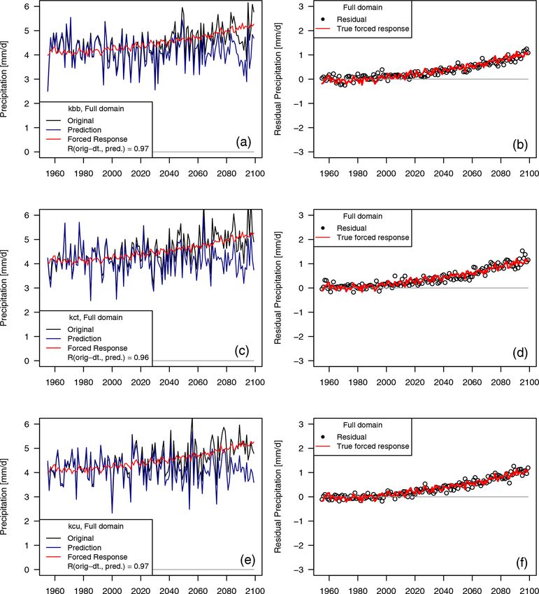
cal adjustment analysis based on the shorter training period Lehner et al., 2017, 2018, for a discussion about trend re-
reveals almost identical results as compared to the longer moval). Here, in addition to the results presented above, we
1955–2070 training period. That is, the residual variability test an alternative simple detrending approach: SLP is not de-
is much closer to the ensemble-mean forced response (see trended, but we detrend precipitation using a simple LOESS
Fig. B3). This sensitivity analysis thus provides support that smoother, fitted on the ensemble (seasonal) means at every
Geosci. Model Dev., 14, 4977–4999, 2021 https://doi.org/10.5194/gmd-14-4977-2021You can also read