Physically based Simulation of Twilight Phenomena
←
→
Page content transcription
If your browser does not render page correctly, please read the page content below
Physically based Simulation of Twilight Phenomena
JÖRG HABER        MARCUS MAGNOR                    HANS-PETER SEIDEL
MPI Informatik, Saarbrücken, Germany

We present a physically based approach to compute the colors of the sky during the twilight period before sunrise and after
sunset. The simulation is based on the theory of light scattering by small particles. A realistic atmosphere model is assumed,
consisting of air molecules, aerosols, and water. Air density, aerosols, and relative humidity vary with altitude. In addition,
the aerosol component varies in composition and particle size distribution. This allows us to realistically simulate twilight
phenomena for a wide range of different climate conditions. Besides considering multiple Rayleigh and Mie scattering, we
take into account wavelength-dependent refraction of direct sunlight as well as the shadow of the Earth. Incorporating several
optimizations into the radiative transfer simulation, a photo-realistic hemispherical twilight sky is computed in less than two
hours on a conventional PC. The resulting radiometric data is useful, for instance, for high-dynamic range environment mapping,
outdoor global illumination calculations, mesopic vision research and optical aerosol load probing.
Categories and Subject Descriptors: I.3.7 [Computer Graphics]: Three-Dimensional Graphics and Realism—Color, Shading,
Radiosity; I.6.3 [Simulation and Modeling]: Applications; J.2 [Physical Sciences and Engineering]: Astronomy, Earth
and atmospheric sciences
General Terms: Algorithms
Additional Key Words and Phrases: physics-based sky model, twilight phenomena, refraction, multiple scattering, 3D radiative
transfer equation

1.   INTRODUCTION
      “The air enwinds the landscape with a wonderful opalescent aura of colors. Without air, light
      and shadow would clash coldly and callously and luridly as they do on the Moon. In all parts of
      the Earth, the colors of the air are the same in their regular as well as divergent appearances.
      . . . The subtle color nuances, the mellow blue, the blue afield, the distance of the sky behind the
      mountains—everything is expressed in a wonderful beauty and a magnificent aura of colors.”
                                                                                         A. Heim (1912)
These lines have not been taken from a poem, but from the introduction to a scientific textbook [Heim 1912].
After this poetic beginning, the author develops a scientific theory of the colors of the sky. Unfortunately, at
that time little was known about the structure and content of the Earth’s atmosphere. Thus, the scientific
relevance of this beautifully illustrated book has turned into a historic one. A similar fate befell another
textbook [Gruner and Kleinert 1927] which describes twilight phenomena such as the bright glow, the purple
light, and the afterglow based on meteorological assumptions that have become—at least partially—obsolete.
Despite the outdated scientific content of these books, the fascination and reverence for the colors of the sky
prevailing in these “historic” documents is still alive and valid today.
   Modern technological advances such as lidar, satellite imaging, and weather balloons have helped to
understand the structure of the atmosphere much better. In addition, precise optical measurements have

Authors’ address: MPI Informatik, Stuhlsatzenhausweg 85, 66123 Saarbrücken, Germany.
Email: haberj@acm.org, magnor@mpi-inf.mpg.de, hpseidel@mpi-inf.mpg.de
Permission to make digital/hard copy of all or part of this material without fee for personal or classroom use provided that
the copies are not made or distributed for profit or commercial advantage, the ACM copyright/server notice, the title of the
publication, and its date appear, and notice is given that copying is by permission of the ACM, Inc. To copy otherwise, to
republish, to post on servers, or to redistribute to lists requires prior specific permission and/or a fee.
 c 20YY ACM 0730-0301/20YY/0100-0001 $5.00

                                                             ACM Transactions on Graphics, Vol. V, No. N, Month 20YY, Pages 1–0??.
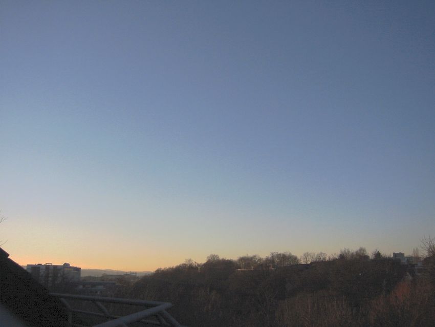
2    ·      Jörg Haber, Marcus Magnor, Hans-Peter Seidel

Fig. 1. Various twilight phenomena simulated with our system for different times and climates. Left to right: horizontal stripes
appear a few minutes after sunset (sun elevation −0.5◦ below the horizon, maritime climate); purple light is at its strongest
about 20–30 minutes after sunset (sun elevation −3◦ , continental climate); afterglow shows up about 40–45 minutes after sunset
(sun elevation −6◦ , continental climate). Nomenclature of twilight phenomena according to [Minnaert 1999].

been performed to determine the scattering properties of air molecules and aerosols. It is due to these two
atmospheric constituents that we perceive the twilight sky in such diverse and changing colors, ranging from
deep blue over all shades of purple, orange, and yellow up to blazing red.
   Rendering outdoor scenes almost always includes vistas of the sky. So far, either actual photographs or
parametric skylight models had to be used for that purpose. But especially for twilight daytimes with their
attractive, quickly changing and diverse lighting conditions, no suitable sky modeling tool has been available.
In particular, for animations of a sunrise/sunset, standard photographs/video cannot reproduce the dynamic
range of the sky while HDR images might be problematic to acquire in the short time of constant sky colors,
and parametric models cannot always deliver the subtle nuances of twilight phenomena.
   The presented work aims at filling this gap by proposing a method to synthesize realistic images of the sky
from its physical causes. It is applicable to any climate, a wide range of meteorological conditions (excluding
only completely overcast skies), arbitrary atmospheric pollution and dust concentration, and specifically to
any time of the day. The output of our system can be used in either of the following ways:
—direct rendering of outdoor scenes;
—computing global illumination for indoor scenes with natural light entering through doors or windows;
—finding optimal parameters for well-known parametric models, e.g. [Preetham et al. 1999; Dobashi et al.
 1997; Tadamura et al. 1993], to achieve realistic sky renderings for a wide variety of atmospheric conditions
 and times of day. This can be achieved by using our physically based simulations as ground truth in an
 optimization approach that computes optimal (non-physically based) parameters for any parameteric
 model by comparision of the predicted result.
Our simulations are based on physical laws in conjunction with physical parameters that have been actually
measured for different climate conditions, taking into account
—solar irradiance spectrum and its absorption in the ozone layer,
—wavelength-dependent refraction of direct sunlight in the atmosphere,
—climate-dependent composition and size distribution of aerosols / dust particles,
—height-dependent air, humidity, and aerosol density,
—Rayleigh scattering (air molecules) and Mie scattering (aerosols),
—radiative transfer (multiple scattering), as well as
—the shadow of the Earth.
ACM Transactions on Graphics, Vol. V, No. N, Month 20YY.

Physically based Simulation of Twilight Phenomena       ·    3

   To calculate the optical characteristics of the atmosphere for any given aerosol mixture, density, particle
size distribution, and humidity, we make use of the publicly available OPAC software package [Hess et al.
1998; Hess 1998] which was originally developed for meteorological and climate simulations.

2.   PREVIOUS WORK
The colorful skies during a cloudless sunset have spurred not only the imagination of countless poets but
also the curiosity of generations of scientists. In a qualitative way, the correlation between twilight colors
and atmospheric conditions has probably been recognized very long ago: country sayings and farmer al-
manacs gave rules to forecast the weather from twilight colors long before the invention of the barometer.
A quantitative explanation, however, eluded even early 20th century scientists [Gruner and Kleinert 1927;
Heim 1912; Minnaert 1999; Rozenberg 1966] who also couldn’t give much more than a description of twilight
phenomena. Today, the underlying physical laws leading to the colors at twilight are well known. A modern,
high-level description of twilight phenomena is given in the textbook by Lynch and Livingston [2001]. Van
de Hulst rigorously derives the scattering characteristics of single particles [1982], and Chandrasekhar’s ra-
diative transfer theory lays the foundation to describe multiple scattering [1950]. Several decades later, the
first computers became powerful enough to enable quantitative investigations of how colors during twilight
depend on atmospheric conditions.
   In essence, we must solve the 3D rendering equation [Kajiya 1986]. Looking for standard radiosity methods,
reproducing faithful twilight colors poses some specific difficulties. First, neither single scattering nor the
diffusion limit are permissible approximations for light transport in the twilight atmosphere [Nagel et al.
1978]: twilight colors are the result of a finite number of multiple scattering events. Second, the atmosphere is
almost transparent, and all regions of the directly illuminated atmosphere receive similar amounts of sunlight.
This renders radiosity methods based on biasing the simulation, for instance importance sampling [Shirley
1990] or progressive radiosity [Cohen et al. 1988], inefficient since all regions are of about equal importance
for the result. Furthermore, an atmosphere volume of tens of millions of cubic kilometers around the observer
contributes to the appearance of the sky. This volume is not orthogonal (due to Earth’s curvature), and
absorption and scattering characteristics vary within the volume. Thus, in direct Monte-Carlo methods, most
simulated photons are wasted, resulting in only sparse distribution information and grainy sky appearance,
even though the actual twilight sky colors vary smoothly [Blattner et al. 1974].
   During the past decades, a large body of literature was published on atmospheric optics. While a lot of
computer experiments were conducted in climatology to investigate global radiative transfer, only a handful
of publications are concerned with the visual aspects of twilight colors, mainly to remotely probe atmospheric
constituents and aerosol density [Bigg 1956; Shah 1970; Jadhav and Londhe 1992; Belikov 1996]. To compute
the radiance observed at a single point on the Earth’s surface during twilight, numerical simulations have
been performed by various authors. Dave and Mateer [1968] show colorimetry results for five atmospheric
models, but do not take into account multiple scattering and atmospheric refraction. The model proposed
by Adams et al. [1974] includes refraction, but still uses single scattering only. Due to the early year of
publication, results are presented as tables and diagrams rather than visualizations. Some early attempts at
simulating twilight phenomena can also be found in the applied optics and planetology literature [Blattner
et al. 1974; Anderson 1983].
   In computer graphics, a number of researchers have concerned themselves with realistic sky visualization.
A system to render the night sky in all its splendor was presented by Wann Jensen et al. [2001]. For daylight
sky rendering, two different approaches have been pursued [Sloup 2002]: phenomenological models describe
sky appearance in terms of non-physical parameters, while physics-based systems solve the 3D rendering
equation known as radiative transfer based on actual atmospheric conditions. An analytical model that can
be fit to actual observational data or simulation results of daytime sky appearance is presented in [Preetham
                                                             ACM Transactions on Graphics, Vol. V, No. N, Month 20YY.
4    ·     Jörg Haber, Marcus Magnor, Hans-Peter Seidel

et al. 1999]. A series expansion of specific sky data was proposed by Dobashi et al. [1997]. Similarly, steerable
basis functions were employed in [Nimeroff et al. 1996]. Tadamura et al. use a skylight model for outdoor
renderings [1993]. These empirical sky light models typically rely on actually recorded images of the sky or
use the CIE standard on daylight luminance distribution [CIE-110-1994 1994]. Their goal is to provide fast
algorithms for rendering a subjectively plausible day or nighttime sky.
   To compute accurate sky appearance from its physical causes, Klassen describes atmospheric scattering
and refraction in suitable form for numerical simulations [1987]. Irwin presents results for a system that
considers Rayleigh scattering from air molecules [1996]. Anisotropic scattering from aerosols is taken into
account by Nishita et al. [1996] as well as by Jackel and Walter [1997]. Both papers also take double
scattering into account. Nishita et al. [1996] employ the two-pass method first formulated by Kajiya and
Herzen [1984]. Their approach is built upon the work by Rushmeier and Torrance [1987] and Max [1994].
Jackel and Walter [1997], on the other hand, introduce an extinction correction term and use a simplified
second-order scattering model. While both papers also present results for times when the Sun is below the
horizon, these images must be considered a rough approximation to the true sky colors after sunset. To
obtain the correct sky illumination during twilight, among other things, higher-order scattering events need
to be taken into account [Blattner et al. 1974; Anderson 1983; Ougolnikov and Maslov 2002].
   We describe an approach how to compute the full radiative transfer in the atmosphere within reasonable
computation times to correctly model all effects that influence sky appearance when the Sun is above as well
as below the visible horizon. This work intends to fill the gap between realistic/physical daytime [Preetham
et al. 1999; Nishita et al. 1996] and night [Wann Jensen et al. 2001] sky rendering.

3.   OVERVIEW
Computing the colors of the sky for an arbitrary observer position and observation date and time is performed
in five steps:
(1) Compute the position of the Sun from the observer position and the observation date and time.
(2) Set up the atmosphere model and initialize all wavelength-dependent optical parameters.
(3) Compute the direct illumination contribution of the atmosphere from the Sun taking into account atmo-
    spheric refraction, the ozone layer, and the shadow of the Earth.
(4) Compute the indirect illumination contribution by simulating multiple scattering events.
(5) Convert the illuminated atmosphere into an RGB “sky texture” as seen from the observer.
  Astronomical Computations. We compute the position of the Sun according to the observer’s longitude
and latitude and the date and time of the observation using the expressions given in [Meeus 1988; 1999].
Similar formulas have been presented by Wann Jensen et al. [2001].
  Setting up the Atmosphere. Our atmosphere model consists of atmosphere layers and atmosphere cells
(Section 4.1). All computations are performed for a number Nλ of wavelengths λi set by the user. Wavelength
samples need not be distributed equidistantly over the color spectrum. Typically, we specify eight samples
covering the wavelength range of visible light (380 nm – 720 nm). We precompute for each wavelength the
optical parameters of the atmosphere using the publicly available OPAC software package (Section 4.1.1).
Spectral solar irradiance (Section 4.2), ozone absorption (Section 4.3), local index of refraction (Section 4.4),
scattering by air molecules (Section 4.5.1) as well as extinction, scattering, and scattering anisotropy due to
aerosols (Section 4.5.2) are taken into account. For tabulated parameter values, we linearly interpolate the
corresponding value for each wavelength λi from neighboring entries in the tables.
  Direct Illumination. All atmosphere cells not in the shadow of the Earth receive direct sunlight (see
Section 4.1). Solar irradiance (Section 4.2) is filtered by the ozone layer (Section 4.3), refracted by air
ACM Transactions on Graphics, Vol. V, No. N, Month 20YY.
Physically based Simulation of Twilight Phenomena       ·    5

molecules (Section 4.4), and scattered by air molecules and aerosols (Section 4.5) on its way through the
atmosphere. After this initial step, each atmosphere cell that does not lie in the shadow of the Earth stores
the radiant power it has received from the Sun.

   Indirect Illumination. This stage takes into account multiple scattering between atmosphere cells (Sec-
tion 4.5.3). It is by far the computationally most expensive step. A naı̈ve implementation can easily exceed
computation times of several days. In Section 5 we thus present several algorithmic optimizations and per-
missible approximations to reduce the computation times for images such as the ones shown throughout this
paper to about 1–2 hours.

   Sky Texture. Finally, we create a sky texture, equivalent to an environment map, which holds the colors
of the sky as seen from the observer’s position in any direction of the hemisphere (Section 4.7). For final
rendering, the spectral information is converted to RGB color space. We convert the sampled spectral distri-
bution into its corresponding XYZ color by convolution with the CIE (1964) 10 ◦ color matching functions.
Next, we convert from XYZ to RGB color space using the sRGB primaries from CIE Rec. 709 and a D65
whitepoint. Details of spectral conversion can be found in [Wyszecki and Stiles 1982] or in [Hall 1989].

4.    SIMULATION
In this section, we describe the physical and meteorological background of our simulations and give details
on the implementation. For an efficient implementation, however, several optimizations have to be included.
These optimizations are described in Section 5.

4.1   Atmosphere Model
Our atmosphere model consists of two sets of distinct building blocks: a set of atmosphere layers and a
set of atmosphere cells. Atmosphere layers are used to store optical properties of the atmosphere, while
atmosphere cells are used during radiative transfer computations.

   4.1.1 Optical Characteristics. The optical properties of the atmosphere depend in a non-trivial way on
climate conditions, local humidity and altitude. We do not attempt to model these complex relationships
ourselves. Instead, we use the publicly available OPAC software package [Hess 1998], described in detail
in [Hess et al. 1998], to compute the wavelength-dependent aerosol absorption coefficient σ aaerosol (λ), scat-
tering coefficient σsaerosol (λ), and anisotropy factor g(λ) (see Section 4.5). OPAC computes these optical
properties for any arbitrary aerosol composition, particle size distribution and humidity. Typical aerosol
mixtures and height profiles for a variety of different climates are also provided by OPAC. At sea level,
the aerosol extinction coefficient σeaerosol (λ) = σaaerosol (λ) + σsaerosol (λ) typically ranges from 0.02–0.4 km−1 ,
while the anisotropy factor g varies between 0.5–0.8.
   The wavelength-dependent scattering coefficient of air molecules is taken from tables in [Nagel et al. 1978].
Unlike aerosols, pure air does not significantly absorb visible light. Thus, the extinction coefficient of air σ eair
can safely be assumed identical to the scattering coefficient, σeair (λ) = σsair (λ). The local index of refraction
of the atmosphere is computed as described in Section 4.4.

  4.1.2 Atmosphere Layers. We model the atmosphere around the Earth up to a height of H max = 35 km.
Above this upper boundary of the stratosphere, there are no more particles or sufficiently many air molecules
to affect our calculations, only the ozone layer which simply filters the incoming sunlight. We discretize the
atmosphere into a set of geocentric atmosphere layers Li , (i = 1, . . . , N ). Each layer Li has an individual
upper and lower boundary at height Hi,max and Hi,min , respectively, with no gaps between adjacent layers:
                                                               ACM Transactions on Graphics, Vol. V, No. N, Month 20YY.
6    ·     Jörg Haber, Marcus Magnor, Hans-Peter Seidel

                                                                                                35 km

                  Hi,max
                       Li                                                  stratosphere
                  Hi,min             air molecules

                                                                                                12 km
                                                                           troposphere
                                                                                                2−10 km
                                     aerosols + air molecules              aerosol layer
                                                                                                0 km
                                                           Earth

Fig. 2. Cross-section of the atmosphere model with atmospheric layers (dotted lines). Decomposition into aerosol-containing
region, clear troposphere, and stratosphere according to [Hess et al. 1998]. The height of the aerosol region depends on the
climate.

Hi,min = Hi−1,max , (i = 2, . . . , N ), see Figure 2. The thickness Di and center height Hi∗ of layer Li then is
                                                              1
                             Di = Hi,max − Hi,min ,             Hi∗ =
                                                                (Hi,max + Hi,min ) .
                                                              2
Each layer Li is assigned a relative humidity wi and the following optical attributes:
                                  aerosol                                 aerosol        aerosol        aerosol
—aerosol scattering coefficient σs,i      (λ) and extinction coefficient σe,i     (λ) = σs,i     (λ) + σa,i     (λ);
—Henyey-Greenstein scattering anisotropy coefficient gi (λ);
                                            air
—isotropic scattering coefficient of air σs,i   (λ);
—index of refraction ηi (λ).
These parameters are functions of the wavelength λ and are evaluated for a discrete set of λ j , (j = 1, . . . , Nλ ).
  Discretizing the atmosphere into individual layers Li allows us to model the variation of optical parameter
values with altitude. To account for the exponential fall-off of particle density with height, we compute for
each layer Li the following factors:
                            ziaerosol (Hi∗ ) = exp(−Hi∗ /Z) ,      ziair (Hi∗ ) = exp(−Hi∗ /8) .
For aerosols, the scale height parameter Z depends on the climate and is provided by OPAC. In each layer
Li , we multiply the extinction and scattering coefficients with the corresponding factor z iaerosol and ziair . The
height dependence of the index of refraction is already incorporated in the equations in Section 4.4.
   Since optical properties are assumed constant within each layer Li , we distribute the layers such that each
layer contains approximately the same number M of air molecules:
                   Z Hi,max
                                                    1 HN,max −h/8
                                                       Z
                                       !
                            e−h/8 dh = M :=                     e     dh     ∀ i = 1, . . . , N .
                     Hi,min                        N H0,min
Substituting Hi,max with Hi+1,min , we obtain the recursive definition

                     Hi+1,min = −8 · ln e−Hi,min /8 − M/8 ,            i = 1, . . . , N −1 ,

where the lower height of layer L1 is initialized to zero, H1,min := 0 km, and the top height of the last layer
is set to the upper boundary of our atmosphere model, HN,max := Hmax = 35 km. The computation of the
ACM Transactions on Graphics, Vol. V, No. N, Month 20YY.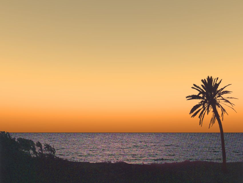
Physically based Simulation of Twilight Phenomena        ·    7

optimal distribution of layers is performed automatically during initialization for a user-specified number of
layers N . For our simulations, we typically use 20–50 layers.
   4.1.3 Atmosphere Cells. Atmosphere cells are set up in the local horizontal coordinate system: the origin
is given by the observer position, and the normal to the Earth’s surface at the observer represents the z-
axis. To be able to later exploit the symmetry of the problem, we let the x-axis always point towards the
azimuthal direction of the Sun. We discretize the atmosphere in small volumes denoted atmosphere cells C k .
These cells are created by uniformly dividing a set of shells along azimuth and height. Shells are located
concentrically about the origin of the local horizontal coordinate system, see Figure 3. In this spherical
parametrization, each cell Ck is described by its spherical coordinates azimuth φk,min/max ∈ [−180◦ , 180◦ ]
height and ψk,min/max ∈ [−90◦ , 90◦ ] and its radius rk,min/max ∈ [R , Rmax ]. Thus, each cell Ck spans the
volume
                          Vk = [rk,min , rk,max ] × [φk,min , φk,max ] × [ψk,min , ψk,max ] .
The spherical coordinates of the center Ck∗ of a cell Ck are set to

                                rk,min + rk,max φk,min + φk,max ψk,min + ψk,max
                      Ck∗ =                     ,                 ,               .
                                       2                 2             2
Any cell whose center is above the Earth’s surface is used for simulation, i.e. also cells below the visible
horizon participate.
  A lower boundary R of the radius has been chosen to avoid cells with a degenerated shape at the origin. In
our simulations we use R = 10m. The upper boundary Rmax is chosen such that the part of the atmosphere
that is still directly illuminated by the Sun during astronomical twilight (i.e. when the Sun is up to 18 ◦
below the horizon) is included in the hemisphere
                                         p            around the observer. With R Earth = 6371 km being the
radius of the Earth we obtain Rmax = Hmax      2  + 2REarth Hmax ≈ 670 km.
  To minimize later approximation errors, we found it beneficial if the atmosphere cells have the same
dimension along radial and vertical direction. We therefore compute the number of shells and the individual
thickness of each shell from a given number S of azimuthal subdivisions. First, we set the identical angular
subdivision for the height (i.e. ψk,max − ψk,min = φk,max − φk,min for all cells Ck ). Next, we compute the
thickness rj,max − rj,min of each shell j to match the average arc length of the (curved) edges of the cells in
that shell (see Figure 4):
                                                              1
                                      rj,max = rj−1,max + (bj−1 + bj ) .
                                                              2
With the arc length defined as bj := α · rj,max , it follows that
                                                   α                    α
                                     rj,max · (1 − ) = rj−1,max · (1 + )
                                                   2                    2
and we obtain the geometric sequence:
                                                               1 + α/2        360◦
                              rj,max = R · q j ,       q :=           , α :=      .
                                                               1 − α/2         S
   We compute and set up as many shells as fit into the interval [R , Rmax ], i.e. until rj,max >= Rmax . In
practice, this mechanism yields 101 shells for S = 72 (5◦ angular subdivision) and 252 shells for S = 180
(2◦ subdivision). This way, we make sure that each cell has the same length in radial as well as height
direction. Cell size, of course, varies strongly between the innermost and the outermost shell, which must
be taken into account during radiative transfer computation.
   During initialization, we store for each cell Ck its center position Ck∗ and volume Vk as well as the index i
of the atmosphere layer Li that contains Ck∗ .
                                                                ACM Transactions on Graphics, Vol. V, No. N, Month 20YY.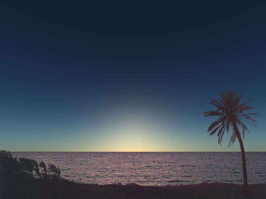
8     ·     Jörg Haber, Marcus Magnor, Hans-Peter Seidel

                                                                   z
                                 z

          ψk,max
                                                 x Rmax           R
      ψk,min
                                                                                                             bj−1      bj
                                                                                        α
                                                                                                          rj−1,max    rj,max
      x
               φk,min                                y
                        φk,max

Fig. 3. Spherical parametrization of our atmosphere model (one quar-         Fig. 4. Cross-section of a single cell with inner
ter of the hemisphere) with color-coded shells. A single atmosphere          radius rj,min = rj−1,max and outer radius rj,max .
cell is drawn with bold lines. Top right: a side view of the xz-plane il-    The arc length of the cell’s curved edges is denoted
lustrates the layout of the shells. The thickness of the shells is adapted   by bj−1 and bj , respectively.
to ensure a relatively uniform cell shape.

   4.1.4 Boundary Conditions. To simulate the propagation of visible light through the atmosphere, we need
to take into account what happens to light that reaches the boundaries of our atmospheric volume model.
For our simulation, we assume that light reaching the boundary of our model volume is lost. This is definitely
true for the upper boundary, since above the stratosphere, no more scattering or absorption takes place, and
light escapes freely into outer space without affecting our simulation anymore. Along the circumference
of our spherical volume lies more atmosphere that contributes some scattered light to our volume, which
we neglect. Two reasons allow us to do so: in daytime regions, the scattered light contribution is many
orders of magnitude dimmer than direct sunlight and thus insignificant; along the twilight border, scattered
outside light affects those regions within the mean scattering length of the atmosphere, while our volume
radius is many times larger than the mean scattering length of the atmosphere; in nighttime regions, outside
atmosphere regions do not contribute at all.
   As the last boundary, the ground remains. The visible-wavelength albedo of Earth’s surface varies con-
siderably, from 3.5% total reflectance for the oceans and 7%-12% for urban areas on to 13% for forests,
15% for farmland soil and up to 90% for freshly fallen snow [Walker ]. Depending on individual ground
conditions around the observer, the effect of sunlight reflected off the ground, or even of scattered sky light
reflected off fresh snow, can have an impact on overall sky brightness, most pronounced during the day.
The ground thereby acts as an undirected area light source, evenly contributing to the illumination of all
atmosphere regions. Thus, if isotropic, wavelength-independent ground reflectance is taken into account, the
relative amount of radiation received by different atmospheric regions does not change considerably. The sky
becomes brighter, but not different in color. So, while our system is easily capable of simulating the effects
of arbitrary Earth albedo characteristics, we decided to present here results for a dark ground.

4.2   Solar Irradiance
For the initial solar irradiance outside the atmosphere we use the solar spectrum data measured by Kurucz et
al. [1984] for wavelengths from 200 nm to 1000 nm. This data is given as spectral irradiance (denoted as resid-
ual flux in Kurucz’s terminology) in Watts per square meter per nanometer (W m −2 nm−1 ) and converted
to irradiance (in W m−2 ) by integrating over wavelength intervals centered equidistantly at 1 nm sampling
ACM Transactions on Graphics, Vol. V, No. N, Month 20YY.
Physically based Simulation of Twilight Phenomena           ·    9

Fig. 5. Left: Spectrum of solar irradiance outside the atmosphere. For wavelength λ ranging from 200 nm to 1000 nm, the
solar irradiance outside of atmosphere is given in W m−2 . Data obtained from [Kurucz et al. 1984]. Right: Absorption of solar
irradiance in the ozone layer for λ = [430 nm, 800 nm]. Outside this wavelength interval, ozone absorption is below 0.1 %. Ozone
scattering coefficients taken from [Nagel et al. 1978].

distance, see Figure 5 (left). We model the Sun as a directional light source, a permissible approximation
since twilight colors vary more slowly with direction than the Sun disc’s diameter of 0.5 ◦ .

4.3   Absorption in the Ozone Layer
The upper part of the stratosphere (at 35 km) contains significant amounts of ozone which filters out the UV
radiation of the incoming sunlight. In addition, ozone exhibits a weak absorption band in the green part of
the visible spectrum. The influence of ozone on the colors of the twilight sky has been studied and simulated
numerically by Adams et al. [1974].
  The ozone present in the stratosphere amounts to a layer of approximately 3 mm thickness at normal
temperature and pressure (20◦ C, 1014 hPa). According to [Royal Meteorological Institute of Belgium 2002],
the thickness of the ozone layer varies periodically between 2.6 mm and 3.7 mm over the year. Taking into
account this annual thickness variation and the wavelength-dependent absorption coefficient σ ozone (λ), we
compute the filtered solar irradiance as:

                                   Ifiltered (λ) = Iunfiltered (λ) · exp (−σ ozone (λ) · d) .

Tabulated values of the ozone absorption coefficient are given in [Nagel et al. 1978]. Figure 5 (right) illus-
trates the effect of filtering by the ozone layer for λ = [430 nm, 800 nm]. Only ozone exhibits non-negligible
absorption in the visible spectrum. Other gaseous atmospheric constituents do not attenuate visible light.

4.4   Atmospheric Refraction
For direct illumination of cells, we take into account atmospheric refraction. Within each layer L i , the
refractive index ηi depends on the wavelength λ, altitude h, and the relative humidity w. In our atmosphere
model, we assume a constant height and humidity within each layer. Thus, for each layer we can precompute
and store the indices of refraction for all wavelengths used during our simulation. To compute η h,w (λ) for
height h and humidity w, we use the following formulas taken from [Ciddor 1996], where the wavelength λ
has to be given in micrometers (µm), the height h in kilometers (km), and the relative humidity w ranging
from 0 for dry air to 1 for a saturated (wet) atmosphere:
                                                                     ACM Transactions on Graphics, Vol. V, No. N, Month 20YY.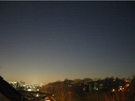
10     ·     Jörg Haber, Marcus Magnor, Hans-Peter Seidel

                                                      Pα
                                     α                                                               center
                           Ck*                                                                       of Sun

                                                                  Atmo−
                                                   Earth            sphere

                                  center of Earth

Fig. 6. Refraction of sunlight in the atmosphere (not to scale). Red line: trajectory without refraction. Blue line: refracted
trajectory is curved downwards and forms an angle α with the unrefracted trajectory.

                ηh,w (λ) = 1 + e−h/8 · ((1−w) · η̃dry (λ) + w · η̃wet (λ))

                                5792105.0          167917.0
                η̃dry (λ) =                  +                    · 10−8
                              238.0185 − λ−2    57.362 − λ−2

                η̃wet (λ) = 295.235 + 2.6422 λ−2 − 0.03238 λ−4 + 0.004028 λ−6 · 1.022 · 10−8
   Several approaches to compute the trajectory of the refracted ray are discussed in Bruton’s disserta-
tion [1996], for instance approximating the trajectory by piecewise parabolas. In contrast, we nonlinearly
ray-trace the path of light through the atmosphere. For a given cell center Ck∗ , we need to find the initial
light direction such that the refracted trajectory ends up traveling towards the Sun, see Figure 6. The
trajectory of light traveling from the Sun to Ck∗ lies in the plane defined by the center of the Sun, the Earth,
and the cell center. 1 . For any given cell, we denote as α the sought angle between geometrical and optical
Sun direction. In practice, this angle is always smaller than 2 degrees.
   We employ a robust and fast iterative algorithm to solve the Eikonal equation (a first order non-linear
PDE, mathematically expressing Fermat’s Principle [Stam and Languenou 1996]) by tracing through the
atmosphere layers Li , given the boundary conditions that the trajectory passes through Ck∗ and ends up in
Sun direction when leaving the atmosphere. For a light ray traveling from layer L i into the neighboring layer
Lj (j = i±1), we compute the direction of the refracted light ray according to Snell’s law of refraction. The
effective index of refraction η used in Snell’s law is the ratio of the indices of refraction η i and ηj of layers
Li and Lj , respectively. For the special case of a sun ray entering the top layer LN of the atmosphere, we
use η = 1/ηN .
   We exploit the fact that due to the decreasing atmosphere density with altitude, the refracted light
trajectory is always curved downward towards the center of the Earth as depicted in Figure 6. The optical
trajectory passing through Ck∗ forms the (unknown) angle α with the straight line connecting Ck∗ and the
center of the Sun CSun . A binary search for α is performed by computing the directional error for a minimal
and maximal angle, initialized with αlow := 0◦ and αhigh := 2◦ . The directional error α is computed as
                                                       D−−−−−→ −  →E
                                          α = 1 − Ck∗ CSun , Pα ,
      −−−−−→                                                                                −
                                                                                            →
where Ck∗ CSun expresses the (normalized) direction vector from cell center to the Sun, and Pα is the (nor-
malized) direction vector of the refracted trajectory at point Pα where it leaves the atmosphere. For the

1 IfCk∗ lies on the line from the center of the Sun to the center of the Earth, the plane degenerates into a straight line and no
refraction occurs since the the light ray penetrates the atmosphere orthogonally.
ACM Transactions on Graphics, Vol. V, No. N, Month 20YY.
Physically based Simulation of Twilight Phenomena · 11
correct value of α, these directions coincide and the error α becomes zero. The binary search typically
converges in 5–15 iterations (depending on the height of the Sun above the horizon) with a remaining error
of 0.1◦ which is considerably smaller than the Sun disc’s diameter of 0.5◦ . Since sky twilight colors vary
slowly with direction, the Sun’s angular extent can be safely neglected, and we assume directed illumination.
At a maximum directional effect of less than 2◦ , refraction is negligible for isotropic as well as anisotropic
re-scattering, which diminishes light directionality.
4.5 Scattering
The splendid colors during twilight are caused by scattering of sunlight by the constituents in the atmosphere.
Colors come about because the amount of scattering varies with wavelength. Since scattering characteristics
depend on particle density, size and material, different atmospheric conditions are responsible for the great
variety of twilight color displays.
Atmospheric scattering effects can be separated into two regimes: Rayleigh scattering caused by air
molecules, which are orders of magnitude smaller than the wavelengths of visible light, and Mie scattering
by aerosol particles (haze, dust, airborne pollutants), whose sizes are approximately of the order of visible
light wavelengths. Atmospheric water content can range from molecular size and droplets in clouds up to
macroscopic rain drops. Excluding rain and fog, the scattering contribution from atmospheric humidity is
already incorporated in the scattering coefficient values calculated by OPAC [Hess et al. 1998].
4.5.1 Rayleigh Scattering by Air Molecules. The molecular constituents of the atmosphere are much
smaller than the wavelength of visible sunlight, and pure air does not absorb any light in the visible regime.
However, the air molecules scatter light, as described by Rayleigh scattering. Each molecule acts as a single
minute dipole antenna which absorbs and re-radiates the very much longer electromagnetic light waves. The
amount of energy first absorbed and then re-radiated in all directions by a single molecule can be analytically
derived from electrodynamic theory [van de Hulst 1982]. Suffice it to state here that the amount of Rayleigh
scattering increases with the fourth power of radiation frequency, i.e. the scattering probability for blue
light is about 16 times higher than for red light. Actually, the perceived blue color of the clear daytime
sky is the result of the combined effects of this fourth-power scattering dependence, the Sun’s spectrum, the
pitch-dark background of empty space beyond our atmosphere, and the photopic response of the human eye
(which prevents us from perceiving the sky as being violet) [Lilienfeld 2004]. For the wavelength-dependent
scattering coefficient of pure air σsair (λ), we use tabulated values taken from [Nagel et al. 1978] which we
scale according to each layer’s air molecule density (proportional to barometric pressure).
The directional characteristics of Rayleigh scattering depend on incident and outgoing light direction, as
well as incoming wave polarization. Since we are concerned here with the appearance of the sky to the
naked human eye, which is by and large not polarization-sensitive, we need to regard only the net effect
on unpolarized illumination. The directional dependence of scattered light intensity is then proportional to
1+cos2 θ, where θ is the angle between incoming light direction and outgoing scattered light direction [van de
Hulst 1982]. This scattering characteristic suggests a darker region in the sky at 90 ◦ from the sun. However,
the clear blue sky appears smooth to the naked eye. This observation already indicates the importance and
the effect of multiple scattering: The scattered blue sunlight is likely to ungo several more scattering events
before reaching the observer on the ground. After the first scattering event, there is no single incoming light
direction anymore. The already scattered light arrives from all directions, diminishing in sum the importance
of angular scattering dependence. The net angular scattering anisotropy evens out very quickly to become
isotropic. Thus, it is safe to approximate the angular dependence of scattering by air molecules as being
isotropic [Nagel et al. 1978]. In Sect. 4.6.2, we make use of this characteristics of multiple scattering again
to efficiently compute multiple scattering events by aerosols.
ACM Transactions on Graphics, Vol. V, No. N, Month 20YY.12 · Jörg Haber, Marcus Magnor, Hans-Peter Seidel
4.5.2 Mie Scattering by Aerosols. A different matter is scattering by particles of sizes on the order of
the incoming light’s wavelength. We use the term aerosols to subsume all kinds of airborne atmospheric
constituents other than molecules, such as soil dust, microscopic water droplets, pollen, minute sulfur beads,
and other solid air pollutants. These particles’ surface acts as if being composed of multiple dipoles that
all oscillate with different phase when excited by an electromagnetic light wave. Particle size, shape, and
dielectric material constant all influence scattering behavior. Mie scattering theory mathematically models
the complex scattering characteristics of such particles. Unfortunately, quantitative descriptions can only be
stated in form of infinite expansion series [van de Hulst 1982]. As general observations, though, Mie scattering
is much less wavelength-dependent than Rayleigh scattering. Instead, it is considerably anisotropic, i.e. light
is preferably scattered into the forward direction.
For our purposes, finding valid approximations to the exact Mie scattering expressions is inevitable. To do
so, we can exploit the fact that we are dealing with a very large ensemble of atmospheric aerosol particles that
is made up of various chemical compounds and a large range of particle sizes and shapes. In addition, the
illuminating sunlight is randomly polarized, incoherent and polychromatic. After averaging the exact Mie
scattering expressions over the range of particle sizes, shapes, and dielectric constants for incoherent light of
arbitrary polarization and a range of wavelengths, the aerosol ensemble’s net scattering characteristics can be
expressed by three coefficients [Hess et al. 1998]: scattering by a mixture of aerosols can be modeled by the
mean scattering and extinction coefficients σsaerosol (λ), σeaerosol (λ), and the mean scattering anisotropy g(λ).
In optics as well as climate research, scattering anisotropy is typically modeled using the Henyey-Greenstein
expression
1 1 − g(λ)2
I(λ, θ) ≈ I1anisotr (λ) · · ∆ω (1)
4π (1 + g(λ)2 − 2g(λ) cos θ)3/2
where θ is the phase angle (i.e. the angle between incident light and scattering direction), g(λ) is the
anisotropy parameter, and ∆ω denotes the scattering cone’s solid angle. σ saerosol (λ), σeaerosol (λ) and g(λ) can
be calculated for any given aerosol mixture, particle size distribution, relative humidity and altitude using
the OPAC software package [Hess 1998].
4.5.3 Multiple Scattering. Twilight colors are substantially influenced by light scattered many times and
over long distances. With the Sun below the horizon, only high-altitude and distant atmospheric regions
in sunset direction still receive direct sunlight. The rest of the atmosphere only receives indirect, multiply
scattered light.
The challenge in simulating the radiative transfer in the atmosphere consists of keeping computation times
as well as memory requirements to manageable levels. Fortunately, as we have seen above, multiple scattering
quickly diminishes the influence of scattering anisotropy. To model multiple scattering through anisotropic
media, it is common practice in optics research [Magnor et al. 2001] to approximate each scattering event as
being isotropic with an effective scattering coefficient
σ aerosol
s (λ) = (1 − g(λ)) · σsaerosol (λ). (2)
In our system, instead of approximating Mie scattering as being isotropic right from the start, we do take into
account anisotropic scattering for the first scattering event. This way, we retain the influence of anisotropic
scattering for the strongest, directional illumination contribution from direct sunlight. Only the indirect,
non-directional illumination from already scattered light is further scattered isotropcially using the effective
scattering coefficient. This approach allows us to accurately simulate the effect of Mie scattering while greatly
reducing computation time as well as required storage capacity, since no directional information must be
stored anymore after the first scattering event.
ACM Transactions on Graphics, Vol. V, No. N, Month 20YY.Physically based Simulation of Twilight Phenomena · 13
4.6 Radiative Transfer
To calculate the distribution of radiant power in the atmosphere, we first need to determine the amount of
direct sunlight received by each atmosphere cell. Subsequently, we simulate the exchange of scattered light
between all cells: We regard each cell as the source cell Csrc that radiates its scattered light towards all other
cells, denoted target cells Ctgt . Two nested loops go over all cells, and it is at this core of our simulation
that the implementation must be as efficiently a possible (Section 5).
For the sake of presentation clarity, in the following we omit explicitly stating wavelength dependency.
4.6.1 Atmospheric Extinction. For cell initialization with direct sunlight as well as during multiple scat-
tering, we need to compute the attenuation of light traveling through the atmosphere layers. Source radiant
power Isrc (λ) (either from the Sun or from a different source cell Csrc ) is attenuated on its way through the
atmosphere such that only a fraction arrives at any target cell Ctgt . The (wavelength-dependent) extinction
factor ξγ (λ) for light traveling along a path γ through the atmosphere is equal to
Z
σeaerosol (λ) + σeair (λ) ds .
ξγ (λ) = exp − (3)
γ
As mentioned in Section 4.1.2, the extinction coefficient of air σeair (λ) is equal to the scattering coefficient
σsair (λ), whereas the aerosol extinction coefficient σeaerosol (λ) also includes a contribution from absorption.
Since atmospheric extinction varies with altitude, each atmosphere layer L i is assigned its individual coeffi-
air aerosol
cient values σe,i (λ), σe,i (λ), and also gi (λ). The light trajectory γ from the source to the target cell is
traced through the layers, and the extinction factor is numerically determined via
N
!
X
air aerosol
ξγ (λ) = exp − σe,i (λ) + σe,i (λ) · ∆γi (λ) , (4)
i=1
where ∆γi (λ) denotes the path length through layer i. Note that, depending on source-target configuration,
typically not all layers are traversed, while, on the other hand, it can happen that a single layer is traversed
twice due to the Earth’s curvature.
To compute the amount of radiant power that is scattered within the target cell C tgt , we compute the
intersection points of the light trajectory γ with the boundaries of Ctgt . Let γfront and γback denote the
paths from the source cell to the front and back intersection points with the target cell, respectively. The
radiant power Itgt (λ) scattered by the target cell Ctgt is then determined by
σs (λ) ωtgt
Itgt (λ) = Isrc (λ) · (ξγfront (λ) − ξγback (λ)) · · , (5)
σe (λ) 4π
with σs (λ) = σsair (λ)+σsaerosol (λ), σe (λ) = σeair (λ)+σeaerosol (λ) being the scattering and extinction coefficients
at the target cell’s position, respectively, and ωtgt denoting the solid angle of the target cell as seen from the
source cell:
r !!!
1 1 Atgt
ωtgt = 1 − cos arctan · .
2 ||Csrc
∗ − C ∗ ||
tgt π
Atgt = Vtgt /(γback − γfront ) is the projected area of the target cell of volume Vtgt . The path length through
each layer ∆γfront (i) as well as the front and back intersection points with the target cell γ front,back is
calculated by efficient ray-plane intersection routines.
4.6.2 Scattering Passes. To consider the first scattering event in the atmosphere, for each cell C k we
calculate the amount of direct solar irradiance reaching the cell according to Equation (4). The amount of
ACM Transactions on Graphics, Vol. V, No. N, Month 20YY.14 · Jörg Haber, Marcus Magnor, Hans-Peter Seidel light scattered inside the cell’s volume by air molecules I1isotr and aerosols I1anisotr is calculated and stored separately (since we model the Sun as a directional light source having irradiance, we substitute for ω tgt /4π in Equation (5) the cell’s projected area Atgt ). This way, each cell is initialized with the radiant power (in physical unit Watts) received from the Sun that is scattered inside the cell. Radiative transfer between all pairs of cells is computed assuming isotropic scattering for the air contri- bution I1iso and anisotropic scattering according to Equation (1) for the contribution from aerosols I 1anisotr . For all possible source-target cell pairs, Equation (5) is evaluated, and both contributions from air and aerosol scattering are combined. At each target cell Ctgt , the radiant power received from all source cells is accumulated to yield I2 of Ctgt . For the next and all higher-order scattering events, the combined effective isotropic scattering coefficient (σ air + σ aerosol ) is used (Section 4.5.3). We repeat calculating the pairwise energy exchange between all cells by now setting I2 as the source cells’ outgoing radiant power. This way, we obtain the contribution to each cell from light that has been scattered three times, I3 . This procedure can be repeated arbitrarily many times to take into account as many multiple scattering events as desired. The simulation time growths linearly with the number of scattering events. To limit memory requirements, it is possible to work with only four buffers per cell: one for the initial anisotropic contribution I anisotr , one for accumulating the total isotropic contribution I isotr , one for the radiant power received during the last pass only I last (needed next time when acting as source cell), and one for gathering the current incoming radiant power I current . After calculating several passes, I isotr contains the amount of radiant power that corresponds to the cell’s equilibrium state between incoming and outgoing light. Thanks to the atmosphere’s relative transparency, I isotr (Ck ) converges quickly to the equilibrium state. Our experiments show that after 5 scattering events, any cell deviates from its equilibrium by much less than 1%, in accordance with results stated in the literature [Blattner et al. 1974; Ougolnikov and Maslov 2002]. 4.7 Creating the Sky Texture We now know for each cell Ck the scattered total radiant power I isotr (Ck ) plus the contribution from direct sunlight that has been anisotropically scattered once by aerosol particles, I anisotr (Ck ). To determine sky colors as seen from the observer’s position, we calculate the radiance scattered from each cell towards an imaginary detector of unit area at the origin. We consider both contributions I isotr (Ck ), I anisotr (Ck ) separately to correctly account for the singly, anisotropically scattered sunlight by aerosol particles. This is important since it turns out that the aerosol-induced forward scattering (g > 0)is responsible for the halo around the Sun. For each hemispherical cell direction (Section 4.1.3), we sum the scattered radiance over all radial shells, taking into account the extinction (Equation (4)) along the path from each cell to the observer. Having completed the simulation run for several wavelengths in parallel, the spectral radiance distribution is converted to RGB [Wyszecki and Stiles 1982]. We have tested different numbers of wavelengths before we decided to settle for 8 wavelengths ranging between 380 nm and 720 nm. The selected wavelengths yield almost exactly the same visual results as if using 16 wavelengths while considerably reducing computation times. We typically run our simulation for a spherical environment map with 3◦ angular resolution. Because sky color varies only slowly with direction, we employ linear interpolation to achieve realistic, high-definition sky textures. Comparative measurements with higher-resolution simulation runs show that virtually no details are lost at 3◦ intervals. ACM Transactions on Graphics, Vol. V, No. N, Month 20YY.
Physically based Simulation of Twilight Phenomena        ·    15

5.   OPTIMIZATIONS
A naı̈ve implementation of the described approach results in huge computation times for each multiple
scattering pass. The main reason for the high computational costs of multiple scattering is the nested loop:
For each (source) cell Csrc of the atmosphere model, we loop over all (target) cells Ctgt and compute the
radiative transfer between source and target cell. The most expensive procedure within the innermost loop
is the computation of the atmospheric extinction along the path from C src to Ctgt (Section 4.6.1).
   To reduce the computational costs of multiple scattering, we can exploit several symmetries. Obviously,
the distribution of radiant power in the “left” and “right” part of the atmosphere model is symmetric w.r.t.
the direction from the observer to the Sun. Thus, we may loop over only half of all source cells and update
two corresponding target cells simultaneously for each source cell. Furthermore, for each pair of one source
cell Csrc and one target cell Ctgt , there is a corresponding pair (Csrc , Ctgt ) for which the path from Csrc to
Ctgt is symmetric to the path from Csrc to Ctgt . Ctgt lies symmetric to Ctgt w.r.t. the plane through Csrc
and the z-axis of the local horizontal coordinate system. Hence, the atmospheric extinction computed for
the path from Csrc to Ctgt can be re-used for the computation of radiative transfer between Csrc to Ctgt ,
allowing Ctgt and Ctgt to be updated simultaneously with only one evaluation of the atmospheric extinction.
Combining the two symmetries described above reduces the number of path computations in the nested loop
to a quarter of the initial number.
   A large reduction in computational cost can be obtained by organizing the loop over all source cells in such
a way that all cells on a ring R of constant height within each shell are regarded successively, i.e. the innermost
source loop runs over the parameter φ from Section 4.1.3. In this case, the paths from any one source cell
of R to all other target cells are identical if the target cell index is shifted corresponding to the source cell.
Thus, we compute all atmospheric extinctions for the first source cell of a ring and store them in a temporary
buffer. For all other source cells of the ring, we use the stored extinction factors instead of re-computing
them. Actually, we store the extinction multiplied by the solid angle (factor (ξ γfront (λ) − ξγback (λ)) · ωtgt in
Equation (5)), since the geometry of the atmosphere model is symmetric about the z-axis. This optimization
reduces the number of path computations by a factor of S, with S being the number of cells in one ring, i.e.
the number of azimuthal subdivisions.
   The above-mentioned optimization steps are purely algorithmic and do not introduce any approximation
errors. To further reduce the computational times of multiple scattering, we make use of the observation
that the computational cost is dominated by the number of shells. We perform multiple scattering only for
a subset of all shells (denoted as active shells) and interpolate the other shells (passive shells). Both loops
over source and target cells benefit from this subsampling. Considering only every n-th shell during multiple
scattering reduces the number of path computations by a factor of O(n2 ). After each multiple scattering
pass, the target cells from passive shells are updated using linear interpolation between their neighboring
cells from active shells. We have to take into account that only a subset of source cells has been regarded.
To ensure a physically correct energy balance, the total amount of energy received by every target cell has
to be scaled by the ratio Iall /Iactive , where Iall and Iactive denote the total radiant energy summed over
all source cells and over the source cells of active shells only, respectively. We regard every fourth shell
during multiple scattering computation, having validated that the obtained results are indistinguishable
from complete-shell simulations. This observation can be understood when considering that the optical
parameters of the atmosphere vary very smoothly along radial direction In addition, the filtering effect of
multiple scattering (diffusion) smears out any localized inhomogeneity.

6.   RESULTS
Our system is capable of calculating accurate sky maps for a variety of different climates, humidities, and
times of the day. All images shown in this paper have been computed with the following parameters:
                                                              ACM Transactions on Graphics, Vol. V, No. N, Month 20YY.
You can also read