Preliminary mission profile of Hera's Milani CubeSat
←
→
Page content transcription
If your browser does not render page correctly, please read the page content below
Preliminary mission profile of Hera’s Milani CubeSat

                                                  Fabio Ferrari∗, Vittorio Franzese, Mattia Pugliatti, Carmine Giordano,
                                                                             Francesco Topputo
                                              Department of Aerospace Science and Technology, Politecnico di Milano, Via La Masa 34,
                                                                               20156, Milan, Italy
arXiv:2102.01559v1 [astro-ph.EP] 2 Feb 2021

                                              Abstract

                                              CubeSats offer a flexible and low-cost option to increase the scientific and tech-
                                              nological return of small-body exploration missions. ESA’s Hera mission, the
                                              European component of the Asteroid Impact and Deflection Assessment (AIDA)
                                              international collaboration, plans on deploying two CubeSats in the proximity of
                                              binary system 65803 Didymos, after arrival in 2027. In this work, we discuss the
                                              feasibility and preliminary mission profile of Hera’s Milani CubeSat. The Cube-
                                              Sat mission is designed to achieve both scientific and technological objectives.
                                              We identify the design challenges and discuss design criteria to find suitable
                                              solutions in terms of mission analysis, operational trajectories, and Guidance,
                                              Navigation, & Control (GNC) design. We present initial trajectories and GNC
                                              baseline, as a result of trade-off analyses. We assess the feasibility of the Milani
                                              CubeSat mission and provide a preliminary solution to cover the operational
                                              mission profile of Milani in the close-proximity of Didymos system.
                                              Keywords: Hera, AIDA, CubeSat, Didymos, asteroid, Milani

                                                ∗ Corresponding  author
                                                  Email addresses: fabio1.ferrari@polimi.it (Fabio Ferrari),
                                              vittorio.franzese@polimi.it (Vittorio Franzese), mattia.pugliatti@polimi.it (Mattia
                                              Pugliatti), carmine.giordano@polimi.it (Carmine Giordano),
                                              francesco.topputo@polimi.it (Francesco Topputo)

                                              Preprint submitted to Advances in Space Research                      February 3, 2021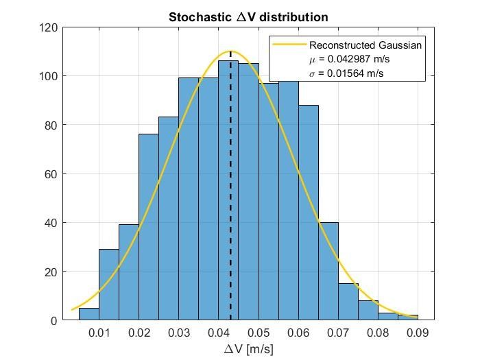
1. Introduction

Motivated by a great scientific interest and large accessibility to space missions,
small celestial bodies represent the current frontier of space exploration. The
close-proximity exploration of asteroids and comets entered a new era in 2000,
as the NEAR-Shoemaker spacecraft entered into orbit around asteroid 433 Eros,
achieving the first rendezvous with a small celestial body (Veverka et al., 2001).
An important milestone was marked more recently, by ESA’s Rosetta (Ulamec
et al., 2014) and later by JAXA’s Hayabusa 2 (Van wal et al., 2018; Tsuda
et al., 2020) missions, which were able to release small probes and SmallSats
on the surface and/or in the close-proximity of such objects. In this context,
CubeSats offer a flexible and low-cost option to increase the scientific and tech-
nological return of small-body exploration missions. Although many concepts of
interplanetary CubeSats have been studied and/or are planned for future mis-
sions (Walker et al., 2018; Franzese et al., 2019; Speretta et al., 2019; Topputo
et al., 2020), very few of them have flown so far (Freeman, 2020; Lockett et al.,
2020), and no CubeSat has ever flown in the proximity of a small-body yet.
ESA’s Hera mission (Michel et al., 2018), the European component of the
Asteroid Impact and Deflection Assessment (AIDA) international collabora-
tion (Cheng et al., 2015), plans on deploying two CubeSats in the proximity
of binary system 65803 Didymos, after arrival in 2027. The idea is supported
by several SmallSat/CubeSat studies that have been performed in the past few
years with reference to Hera (formerly known as AIM), to study the feasibility
of deploying a small lander (Ferrari and Lavagna, 2018, 2016; Lange et al., 2018;
Çelik et al., 2019) and possibly CubeSats (Kohout et al., 2018; Lasagni Manghi
et al., 2018; Perez et al., 2018) in the close proximity of Didymos. These were an-
ticipated by detailed studies of the dynamical environment near binary asteroid
systems (Tardivel and Scheeres, 2013; Tardivel, 2016; Ferrari et al., 2016, 2014;
Çelik and Sánchez, 2017), some with direct application to the Didymos case
study (Dell’Elce et al., 2017; Capannolo et al., 2019, 2016). Hera is currently
in its phase-B design, on-track to be launched in 2024. Its payloads have been

                                        2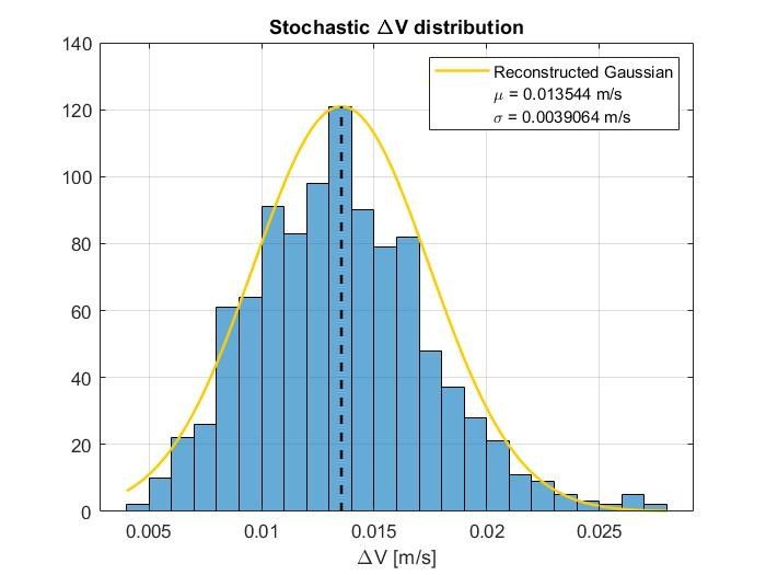
recently consolidated and, as mentioned, it will carry two 6U CubeSats, to be
deployed after rendezvous with Didymos. These are called Juventas (Karatekin
et al., 2019) and Milani. Milani has been officially confirmed on mid 2020 and
is currently in its phase-A design. Its flight readiness does reflect Hera schedule,
foreseen in late 2024.
In this work, we discuss the feasibility and preliminary mission profile of Hera’s
Milani CubeSat. The Milani mission is designed to achieve both scientific and
technological objectives. The first include the global mapping of Didymos (pri-
mary) and Dimorphos (secondary) asteroids. This involves determining the
composition difference between the bodies and the study of their surface prop-
erties. In the context of the AIDA international collaboration, Milani will help
at determining the composition of the ejecta created after the impact of DART
spacecraft (Cheng et al., 2018) in 2022 on the surface of Dimorphos, and their
fallbacks on the surface of the asteroids. In terms of the technological objec-
tives, the mission will be among the first to operate CubeSat technologies in deep
space and the first to use Inter-Satellite Link (ISL) network with the mother
spacecraft in such challenging context.
Milani is a 6U CubeSat with maneuvering capabilities both in terms of trans-
lational and attitude motion (full 6-DOF). After release it will perform au-
tonomous operations to reach its operational trajectories towards the fulfilment
of its mission goals. The main payload aboard Milani is the ASPECT hyper-
spectral camera (Kohout et al., 2018). The characteristics of the ASPECT
camera are reported in Table 1. The payload has three channels, which are
the Visible (VIS), the Near-Infrared (NIR), and the Short Wavelength Infrared
(SWIR). The three channels have different characteristics, especially in terms of
field-of-view and sensor size. These quantities affect the allowed orbital ranges
to the targets for scientific observations. The visible channel has the largest field
of view and a 1 Mpx sensor size. The NIR is narrower than the VIS channel,
while the SWIR is a mono-pixel circular FOV channel. In addition to ASPECT,
which is used for scientific imaging only, Milani hosts two additional cameras,
which are used for optical navigation. These cameras have not been selected yet:

                                          3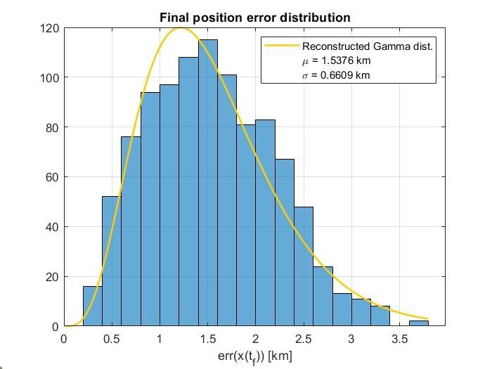
Table 1: Characteristics of the ASPECT hyperspectral camera.

         Parameter         Unit         VIS              NIR        SWIR

         Field-Of-View      deg        10 x 10      6.68 x 5.36        5
         Sensor Size        pix     1024 x 1024        640 x 512       1
         Pixel Size         µm        5.5 x 5.5         15 x 15      1000
         Focal Length       mm           32.3            81.7        11.7
         F-number             -          3.3              6.0         0.9

the properties and performance assumed for navigation cameras are reported in
Section 4.4. As a seconday payload, Milani hosts the VISTA thermogravime-
ter (Dirri et al., 2018), which will collect information on the dust environment
near the asteroids. It is operated in background during the operational phases
of the Milani mission: it does not impose any further requirement and does not
require a specific tayloring of the mission profile.
After release in the proximity of Didymos binary asteroid, Milani independently
makes its own way to its operational trajectory, optimized to observe the aster-
oid system. In this work, we consider the CubeSat limitations given by minia-
turized components, and address the challenges in deriving an optimal mission
profile which meets the mission and scientific objectives. The GNC architecture
and design that allow to achieve such a mission are also shown. It is worth
stressing that the initial results presented in this paper have been obtained in
response to the relevant ESA call. As such, the preliminary profile here shown
will be revised as both mission and spacecraft design advance in later stages.
The paper is organized as follows. Section 2 reports the design constraints
of the mission given by the environment and the payload. Section 3 shows
the mission profile with a detailed explanation of the mission phases. Then,
the GNC architecture and preliminary design are shown in Section 4. The
operational analysis of the payload is reported in Section 5. Finally, conclusions
and a summary of the results are given in Section 6.

                                          4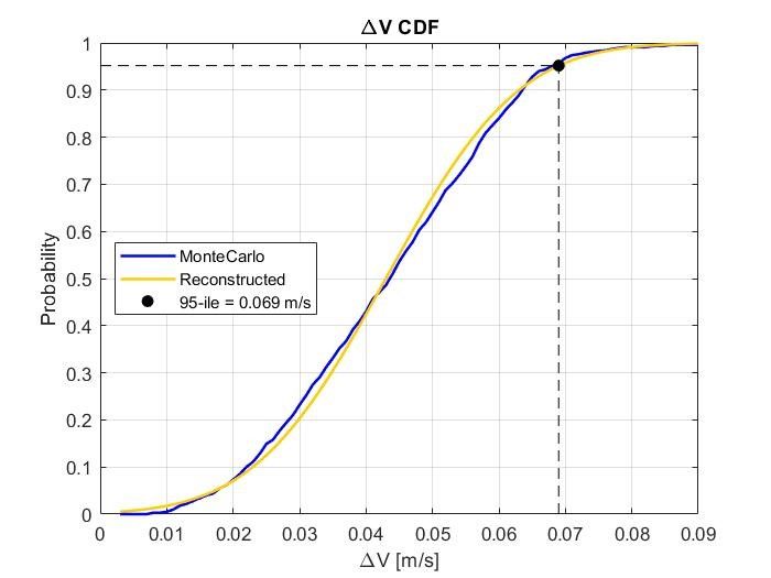
Table 2: Didymos system characteristics and imaging constraints.

   Asteroid         d        md      pv          GSD            α         θ/FOV

   Didymos       780 m     10 %     0.15       ≤ 2 m/pix   5 – 25 deg         ≤4
   Dimorphos     170 m     10 %     0.15       ≤ 2 m/pix   5 – 25 deg         ≤1

2. Design constraints

The constraints affecting the design of the mission and the CubeSat platform
are presented in this Section. The Didymos binary system is composed of two
asteroids: the primary (Didymos, also called D1 in the following) and its satel-
lite (Dimorphos, also called the secondary or D2 in the following). The primary
body has an estimated diameter of 780 m and an assumed albedo of 0.15. The
secondary has an estimated diameter of 170 m and an assumed albedo of 0.15.
Current estimates consider a 10 % size error for both asteroids. The require-
ments applicable to the Milani CubeSat derive directly from both the mission
objectives and the ASPECT payload. To achieve the mission objectives with
ASPECT, the payload team has determined the following two main conditions:
1) To map both asteroids with a ground resolution lower than 2 m/pixel with
images from both the VIS and the NIR channels; 2) To observe the asteroids
with a phase angle (Sun-asteroid-CubeSat angle) between 5 and 25 degrees.
In order to ease the operations of Milani, Dimorphos is required to be imaged
within a single picture, always inside the FOV of ASPECT, while the primary
can be imaged as a 4-images mosaic. These values are summarized in Table 2,
where d is the equivalent diameter of the asteroids, md the associated margin, pv
the albedo, GSD the ground sampling distance, α the phase angle, and θ/FOV
the ratio between the apparent dimension of the asteroid to the ASPECT field-
of-view. Note that the limiting value for the FOV is given by the NIR channel,
since it is narrower than the VIS channel. The SWIR channel is not considered
here because it is a monopixel channel.
With the values in Table 2, it is easy to verify that Dimorphos fills the FOV

                                           5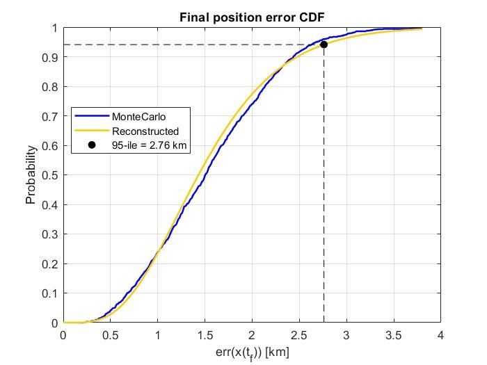
of the VIS channel at 1069 m of distance and the FOV of the NIR channel
at 1997 m of distance, while Didymos fills a 2×2 image mosaic using the VIS
channel at a distance of 2433 m and the NIR channel at 4572 m. Thus, the
value of 4572 m is considered as the lower bound on the range constraints to the
binary system. The maximum allowable ranges to meet the 2 m/pix imaging
GSD are 11700 m for the VIS channel and 10940 m for the NIR channel. Thus,
the upper bound on the relative range between the binary system and Milani is
10940 m. The communication link between Milani and the mother spacecraft
through the ISL is assumed to be omnidirectional and available up to 60 km of
relative distance between the two spacecraft.
All in all, the operations in the nominal orbit shall be performed at ranges from
Didymos within 4572–10940 m and phase angles within 5 and 25 degrees, as
summarized in Table 3, within a 60 km range from Hera mothercraft.

                         Table 3: Mission design constraints.

 Asteroid     Min Range      Max Range        Min Phase Angle   Max Phase Angle

 Didymos        4572 m         10940 m              5 deg             25 deg

3. Mission profile

This section presents the preliminary mission profile for Hera’s Milani CubeSat,
from its release in the proximity of Didymos system, up to its decommisioning.
We discuss the design strategy to provide efficient release of Milani from Hera
spacecraft and detail the operational trajectories during the CubeSat science
phase. End-of-life options are proposed. The feasibility of the mission profile is
eventually discussed. The overall design is compliant with constraints outlined
in Section 2. The dynamics of the CubeSat near the Didymos system are studied
using a high-fidelity model, which includes the heliocentric motion of Didymos
system barycenter, the binary motion of the asteroids (provided by high-order

                                          6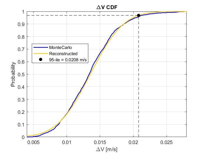
integration in ESA’s Hera Mission kernels1 ) and relevant perturbations, such
as the effects of the non-sphericity of asteroids (through a polyhedral model
of Didymos and ellipsoidal model of Dimorphos) and Solar Radiation Pressure
(SRP).

3.1. Release strategy

The Hera spacecraft plans on releasing Milani after arrival at Didymos system,
in late spring 2027. In this work, we set the release date to May 1st, 2027. At
this time the Didymos–Sun distance is 1.5 AU and increases up to 2.0 AU during
the expected operational life of the CubeSat. The selection of Milani operational
dates is important to characterize the dynamical environment in the proximity
of Didymos, as it affects the magnitude of the SRP, which is relevant. On the
other hand, the release date does not affect the operations of Milani in terms
of orbital determination and illumination conditions. The relative geometry of
Hera trajectories and release point is set in terms of Milani/Hera, Didymos and
Sun position. At any epoch, the release will be performed when Hera is between
the binary system and the Sun direction, in order to have Didymos visible on
its day side. Milani’s release conditions are carefully selected after an extensive
analysis, involving the investigation of different release points on Hera’s Early
and Detailed Characterization Phases trajectories 2 , the analysis of geometrical
constraints at release, the dynamics of the CubeSat after release relative to Hera
mothercraft and Didymos system. In particular, the following criteria have been
considered in terms of release geometry and release trajectory:

   • Minimum angle between CubeSat release velocity direction and CubeSat-
       Sun direction of 45 deg;

   • Minimum safety factor C of the release trajectory of 0.4.

  1 https://www.cosmos.esa.int/web/spice/data,    Last accessed: June 2020
  2 see   Hera Mission kernels documentation at https://www.cosmos.esa.int/web/spice/
data

                                           7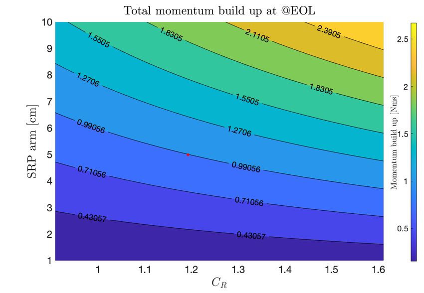
The safety factor C measures the energy of the trajectory (C>0 for hyperbolas),
and is defined as
                              vperi = (1 + C)vparab                           (1)

with vperi and vparab defined as the velocity at pericenter on the release trajec-
tory and the parabolic velocity at the release point, respectively. These con-
ditions derive from the mother spacecraft requirements in terms of safety and
illumination conditions. In addition, the release trajectory was selected to guar-
antee consistent relative motion with respect to Hera spacecraft and Didymos
system for up to 7 days after release, in terms of:

   • Maximum CubeSat–Hera distance of 60 km, to ensure communication
     with the mothercraft;

   • Maximum phase angle of Didymos system (Sun-Didymos-CubeSat angle)
     of 90 deg, to ensure dayside visibility of the asteroids;

Finally, we analysed the robustness to release uncertainties, related to both the
deployer mechanism and Hera’s GNC accuracy. These are quantified as:

   • Release velocity in the range 0-5 cm/s (±1 cm/s, 3σ value)

   • Release direction accuracy of the deployer mechanism within 5 deg (3σ value)

   • Release orientation accuracy of Hera spacecraft within 0.5 deg (3σ value)

The analysis performed is aimed at finding suitable release directions. In this
case, pointing and release direction errors are the most important sources of
errors. Position and velocity errors of Hera play a minor role in detecting pre-
ferred directions and, at the current stage they can be neglected. These will be
added at a later refinement of the design. Release points are chosen among Hera
spacecraft trajectories, which are retrieved from ESA’s Hera Mission kernels.
We performed an extensive Monte Carlo analysis of the parameter space (40k
runs among eight difference release points) and, as a result, a release from
30 km (distance from Didymos system barycenter) in the direction (Az=10 deg,
el=60 deg), is selected as a design baseline solution. Directions are shown in

                                        8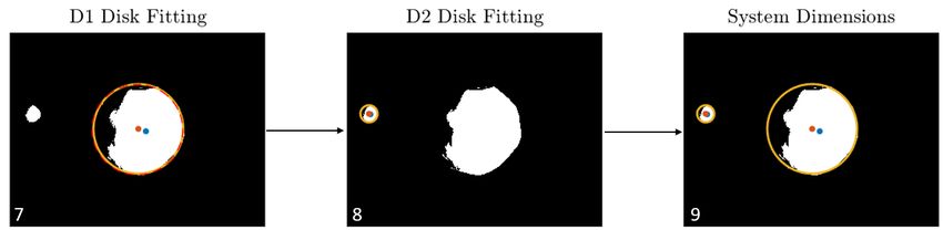
Didymos equatorial plane, where Azimuth is the in-plane angle (Az=0 deg to-
wards the projection of Sun’s position on Didymos equatorial plane), and ele-
vation is the out-of-plane angle. Figure 1 shows the results of the analysis in
terms of release direction, for the 30 km distant release point. Each release
condition is propagated forward for 7 days. The compliance to the aforemen-
tioned constraints is checked at any time on the release trajectory. Feasible
release directions are identified by green markers, while red markers indicate
conditions where the constraints are not satisfied. Unfeasible release direction
in Figure 1 are characterized by a mix of green and red markers. This is due
to effect of the release velocity: these directions are typically unfeasible for high
release velocities (close to 5 cm/s), but might be feasible for lower velocities. In
fact, the higher the release velocity, the higher the probability of falling beyond
a 90 deg phase angle or 60 km distance from Hera after a 7-day ballistic arc.
The blue marker highlight the selected release direction.
The release solution is shown in Figure 2. The trajectory of Milani and Hera
spacecraft are shown for seven days after release. This solution is compliant
with design constraints, robust to uncertainties, and guarantees a safe 7-day
ballistic arc after release.

3.2. Operational trajectories
After release from Hera and commissioning, Milani will maneuver to perform
scientific operations. This section presents the selected operational orbit and
maneuvering strategy to accomplish Milani’s mission objectives. As summa-
rized in Table 3, scientific operations are carried at a distance within the range
4.572-10.940 km from Didymos system and when the phase angle (Sun-asteroid-
CubeSat angle) of Didymos and Dimorphos is in the range 5-25 deg. Also, we
enforce the CubeSat to have a non-zero elevation above Didymos equatorial
plane, to ensure visibility of the asteroids poles. In terms of ∆v cost, we consid-
ered a budget of 10 m/s. In addition to constraints reported above, additional
design drivers were considered, namely:

   • Safety, in terms of orbital energy, quantified by the safety factor C. We

                                         9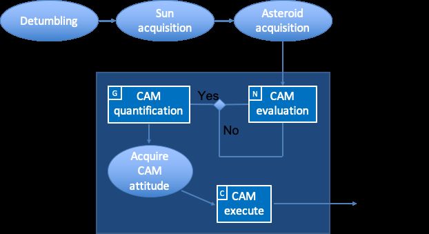
Figure 1: Release options in the Didymos equatorial plane. Green and red markers indicate
compliant and non-compliant solutions, respectively. The upper-left picture is the composite
of the other three pictures, plus the addition of geometrical constraints at release (forbidden
±45 deg cone around CubeSat-Sun direction).

   Azimuth is the in-plane angle (Az=0 deg towards the projection of Sun’s
  position on Didymos equatorial plane), elevation is the out-of-plane angle.
   Yellow and black markers indicate the direction of the Sun and Didymos,
 respectively, as seen from the release point. The blue marker represents the
                               selected release direction.

      give the highest priority to trajectories that are inherently safe, i.e. with
      C>0 (hyperbolic arcs). Closed trajectories (C
Figure 2: Nominal release trajectory in the Didymos equatorial frame. Milani’s and Hera’s
orbital motion is shown for seven days after release. Geometrical constraints (release exclusion
angle around Sun’s direction), and Didymos system are shown.
• Robustness to uncertainties due to the system and dynamical environ-
ment. This is tightly connected to safety and simplicity criteria. Inher-
ently safe trajectories are typically more robust to uncertainties. On the
other hand, long ballistic time of flights between consecutive manoeu-
vres require robust trajectories, able to deal with uncertainties without
jeopardizing the safety of the Hera mission or altering the mission profile
strategy.
• Cost, in terms of ∆v. Our analyses show that cost is not critical to our
mission. For this reason, safe, simple, and robust trajectories are preferred,
at a cost of a slightly higher ∆v.
We performed an extensive trade-off analysis between several orbital strategies
and trajectory solutions, including hyperbolic arcs, closed orbits and three-body
11proximity solutions. The results of the trade-off are summarized in Table 4. In
particular, we show the suitability of each strategy in terms of available time for
science operations (time in the science admissible region), navigation constraints
(check on phase angles and asteroid illumination), safety/risk of entering chaotic
dynamics, simplicity of operations/maneuvering strategy, dynamical robustness
to uncertainties and ∆v cost. The study clearly identifies the hyperbolic-arc
strategy as the most promising solution to host Milani scientific operations.
This has several advantages in terms of safety, simplicity and robustness, and
provides the best option in terms of asteroid visibility. In particular, we imple-
mented a patched-arc manoeuvring strategy that leverage the SRP acceleration
to target pre-selected waypoints. To reduce the burden for active operations, we
consider a 4-3-4-3 maneuvering pattern, where maneuvers are performed after
a 4- or 3-day ballistic arc. This is similar to the strategy implemented by the
Hera spacecraft. Selecting such pattern has the advantage to ease operations at
maneuvering points, which will be fit within a fixed weekly schedule and aligned
to Hera operations.
After a thorough design process, where several hyperbolic-arc waypoint configu-
rations have been investigated, the waypoints of the hyperbolic loop are selected
as shown in Figure 3. Left plots in Figure 3 show the ranges and admissible
science regions (between dashed lines). Milani has science windows of 1-2 days
for each arc. Projections of the trajectory on the Didymos equatorial plane are
shown on the right. To maximize the time spent by the spacecraft within the
science admissible region, the orbital plane between consecutive hyperbolic arcs
is tilted by a few degrees at each maneuvering point. This is clearly visible in
the y-z projection plot (lower-right). This allows Milani to fly within admissible
ranges in terms of aspect angle and distance, when transiting near the pericen-
ter of each hyperbola. Numbered labels indicate the maneuver sequence, under
the 4-3-4-3 day scheme, from maneuver 0 (insertion into science loop trajectory)
up to maneuver 5. The waypoint design strategy is modular and can be fur-
ther extended. As detailed in Section 5, six hyperbolic arcs (21 days in total)
are enough to accomplish the scientific objectives of the mission. If needed,
12Table 4: Science orbit trade-off matrix.
Strategy Time for Navigation Safety/risk Simplicity Robustness Cost:
science monthly
Loop 1-2 days Always on Inherently Compliant 3-4 days 1.5 m/s
(C>0) per loop asteroids’ safe to 4-3-4-3
dayside pattern
Loop 2-3 days Always on Moderate Compliant 2-3 days 1.2 m/s
(CFigure 3: Nominal science trajectory. Phase angle and distance time profile with respect to
Didymos (D1) and Dimorphos (D2) are shown in upper and lower left plots. Science admissible
region is highlighted (ranges between dashed lines). Projections on Didymos Equatorial frame
x-y and y-z plane are shown in upper and lower right plots, respectively. These show science
admissible regions in terms of distance from the binary system (green sphere is minimum
distance, red sphere is maximum) and phase angles (green cone is minimum value, red cone
is maximum value). The Sun direction is also shown (orange arrow inside the green cone), as
well as the projection of Hera spacecraft’s trajectory (green lines in the upper right plot).
discussed, the nominal science loop is built as a sequence of hyperbolic arcs.
Missing one manoeuvre would safely bring Milani into an escape trajectory
from the Didymos system. In addition, the SRP accelerates the CubeSat further
away from Didymos, increasing its orbital energy. In this case, a safe graveyard
heliocentric orbit can be achieved by missing the last manoeuvre of the scientific
phase. After this, the spacecraft takes approximately 10 days to fly beyond a
60 km distance from Hera spacecraft. This option is the safest possible and
may be preferred to avoid criticalities in terms of operational burden and costs.
However, it does not provide any opportunistic science information in addition
to those gathered during the science phase: it is a low risk-low gain solution.
14Option 2: Landing attempt on Dimorphos. The second option is to attempt
a landing on D2. After the nominal scientific and technological objectives of
the mission are accomplished, it might be worth to exploit Milani to provide
additional data on the Didymos system. To achieve this goal, a higher risk
can be accepted. In this context, we plan to get closer to the Didymos system,
dropping the design driver of flying inherently safe hyperbolic trajectories. As
mentioned, orbiting the inner region of Didymos system poses several challenges
in terms of navigation and robustness to manoeuvres. This is a high risk-high
gain option. The knowledge analysis performed in Section 4.2 shows that, in
principle, the current GNC baseline would be compatible with a soft-landing
design for the CubeSat. However, a more detailed analysis will be required to
rigorously assess the feasibility of such option.
3.3. Momentum budget
As mentioned, the SRP plays a fundamental role in assessing the dynamics
of the CubeSat in the close-proximity of Didymos. Also, it contributes in a
relevant manner to the active maneuvering costs to be provided to control the
attitude of the CubeSat. The momentum budget is estimated here by assessing
the impact of the SRP perturbation to the attitude dynamics of Milani. We use
a cannonball model with an equivalent area of 0.5160 m2 , a reflection coefficient
(Cr ) of 1.1926, and a constant arm of 5 cm. These data are consistent for a 6U
CubeSat with large solar arrays.
As mentioned earlier, the baseline scenario considers that Milani is released in
May 2027, when the distance from the Sun is 1.5 AU, reaching 1.9 AU and
2.2 AU after 3 and 6 months of operations, respectively. For comparison, we
consider here the backup launch option as well, which considers a CubeSat
release on January 2031, when the distance from the Sun is 1.1 AU, reaching
1.5 AU and 1.9 AU after 3 and 6 months of operations, respectively. The latter
option is considered since it is a worst case scenario: the CubeSat is closer to
the Sun and the effect of SRP is higher. The total momentum buildup due to
SRP in the worst case scenario (backup launch and 6 months of operations)
15Figure 4: SRP total momentum build up by the SRP on Milani after 6 months. The nominal
value is shown with a red marker for CR = 1.19 and SRP arm=5 cm.
is illustrated in Figure 4 as function of the key parameters of the cannonball
model. With the nominal values a total momentum build up of 0.99 mNms
during the whole mission is estimated.
Assuming that the disturbance torque is building up on a single reaction wheel,
two options are considered in terms of momentum capacity: 25 mNms and
55 mNms. In the first case a total of 40 dumping manoeuvres would be required
for 6 months of operations (approximately 1 manoeuvre every 4.5 days) while in
the latter one the number drop to 18 for 6 months of operations (approximately 1
manoeuvre every 10 days). The total ∆V budget to be allocated for momentum
dumping is therefore estimated to be around 1 m/s in the worst case scenario.
The evolution of the ∆v budget for desaturation as function of the mission
launch and duration is illustrated in Figure 5.
16Figure 5: Desaturation budget as function of mission duration for the nominal launch (blue
curve) and backup launch (red curve).
4. GNC strategy
The key driver for Milani’s GNC subsystem design is to maximize the opportuni-
ties to observe the binary asteroid system. Also, it is paramount to complement
the Orbit Determination (OD) with optical navigation, to always track the tar-
get asteroid, and to increase the efficiency of the operations by exploiting the
pointing of the scientific observations for optical navigation. All in all, it is
beneficial for the mission to never lose the line-of-sight to the target asteroid
while performing scientific but also housekeeping tasks.
The GNC system architecture is shown in Figure 6. Milani is equipped with an
on-board computer (OBC) where two modules are present, namely the ADCS
processing module and the GNC processing module. These modules are re-
sponsible for collecting and processing sensor inputs to elaborate commands for
the actuators. The ground segment is responsible for computing the nominal
guidance, navigation, and control of the satellite. This information is sent to
the Hera spacecraft that is acting as a relay satellite and then sent back to
Milani via the inter-satellite link (ISL). Apart from the ASPECT payload, we
assume that Milani is equipped with a 21×16 deg NavCam and a 40×40 deg
Wide Angle Camera (WAC). These are required for high-resolution imaging of
the asteroids and optical navigation, as described in Section 4.4. The navigation
measurements for Milani come from the navigation camera and ISL. The nav-
17CubeSat
OBC
IMU
Attitude
Sun Sensors
Control
Star Trackers ADCS Processing Module
Reaction Wheels 6 DOF
RCS
Navigation Camera
GNC Processing Module
Orbit
ISL TX/RX Control
ISL link
X-band
RF link
Hera Ground Segment
Figure 6: System architecture.
igation camera is used to acquire images of the two asteroids, while the ISL is
exploited for range and range-rate measurements with respect to Hera. Milani is
equipped with a Six Degree-of-Freedom Reaction Control System (6 DOF RCS)
for trajectory and attitude control. The attitude measurements for Milani are
given by an Inertial Measurement Unit (IMU), two sun sensors, and the star
trackers. The attitude is also controlled by the reaction wheels.
4.1. Guidance
The Differential Guidance (DG) strategy (Dei Tos et al. (2019); Park and
Scheeres (2006)) adopted for Milani’s guidance is detailed in this section. In
the DG formulation, the whole trajectory is subdivided in different legs. At
the extremal points of a single leg, two maneuvers are applied to cancel both
the position and velocity deviations on the final leg point. However, the final
impulse is usually not applied in practice, since at the time of arrival at the final
point a new maneuver is calculated in a receding horizon approach. The ma-
neuver can be computed by minimizing the deviations from the nominal state
18at the final point in a least square residual sense. Thus, the maneuver that has
to be applied at the time tj in order to cancel out the deviations at time tj+1
is computed as Dei Tos et al. (2019)
−1
∆vj = − ΦTrv Φrv + ΦTvv Φvv ΦTrv Φrr + ΦTvv + Φvr δrj − δvj
(2)
where δrj and δvj are the (estimated) position and velocity deviation at time
tj , Φrr , Φrv , Φvr and Φvv are the 3-by-3 blocks of the State Transition Matrix
(STM) Φ (tj , tj+1 ) from time tj to time tj+1 associated to the nominal trajectory.
4.2. Knowledge Analysis
Errors in the dynamical propagation of the trajectories, e.g. inaccuracies in
state determination or thrust misalignment, can lead to large deviations with
respect to the nominal trajectory. Hence, a knowledge analysis is required to
compute, through a covariance analysis, the achievable state knowledge. Sim-
ulations of the radiometric data for range and range-rate coming from the ISL
are performed, generating the pseudo-measurements as
p ρT η
ρ= ρ T ρ + ερ , ρ̇ = + εη (3)
ρ
where ρ is the range, ρ̇ is the range rate, ρ = r − rH is the relative distance
between Milani and Hera, while η = v − vH is the relative velocity with ε rep-
resenting the error. r and v are position and velocity of Milani Cubesat, while
rH and vH represent position and velocity of the Hera spacecraft. Pseudo-
mesaurements are used to feed an Extended Kalman Filter (EKF, Schutz et al.,
2004) in order to simulate a realistic Orbit Determination procedure. In our
case, the Hera spacecraft is always in view and no assessment of visibility win-
dows is needed.
4.3. Guidance & Navigation closed-loop approach
The overall navigation cost, necessary to keep the spacecraft on the nominal
path, is estimated in a closed-loop fashion, taking into account: 1) the knowledge
analysis (as in Section 4.2) to estimate the deviation of the real trajectory from
19the nominal trajectory at the target points; 2) the differential guidance (as in
Section 4.1) to assess the stochastic cost, starting from the estimated deviations.
The total navigation cost is estimated by means of a Monte Carlo simulation.
Following this approach, an initial Gaussian distribution with mean x̄0 and
covariance P0 is identified and a set of samples xi0 is generated. Both the
state and the covariance matrix are propagated with the associated dynamics
up the first measurement epoch, where the estimated trajectory is updated.
Proceeding in this way, the state estimates are sequentially updated as new
measurements are processed, leading to the position and velocity knowledge
profiles. This is repeated up to the final epoch of the Orbit Determination
phase, where the deviation from the nominal path is estimated. The deviation
is then pushed forward using the STM up to the maneuver time and used to
feed the guidance law. The correction impulse is computed and applied. The
whole process is repeated up to the final time for each initial state in the sample
set. The estimation of the total cost for each sample is obtained as the sum of
PN
all maneuvers’ cost, i.e., ∆vi = j=1 ∆vji .
4.3.1. Science phase
During the science phase, it is of paramount importance to acquire precisely
and track the nominal trajectory in order to achieve the mission objectives.
An assessment considering a higher fidelity model, with the OD process in the
loop, is performed. Some assumptions are made for this analysis and they are
listed below:
• The guidance law is the standard differential guidance algorithm;
• Correction maneuvers are given together with deterministic maneuvers;
• No uncertainty in stochastic maneuvers is considered;
• Due to technological constraints, correction maneuvers are not applied if
their value is lower than 5 mm/s;
20• An initial a-priori uncertainty of 10 m on position, 1 mm/s on velocity
(3σ) is used;
• To compensate for differences between physical model and real world, a
thrust misalignment of 1% in magnitude and 1 deg in pointing angle (3σ)
is considered;
• The ISL is simulated taking into account an accuracy of 1 m in range and
0.1 mm/s in range-rate. The error is modelled as Gaussian noise;
• In order to allow Flight Dynamics estimations and reduce the operational
costs, an interval of 1.5 days between the maneuver and the beginning of
the OD phase is considered, while a cut-off time of 1 day is inserted before
the maneuver;
• The ISL performs a range measurement every 20 minutes and a range-rate
every 2 minutes;
• Propagation is done linearly by means of the STM, while the estimation
is done exploiting the EKF;
• 1000 samples Monte Carlo run.
Following these assumptions, a timeline for the science orbit can be derived. In
Figure 7, red dots indicate when the range measurements are computed, while
blue dots shows range-rate measurements. Orange bars mark the maneuvers
time.
The outcome of the knowledge analysis is reported in Figure 8 and Figure 9.
They illustrate the results of the covariance analysis and, in particular, the
achievable knowledge accuracy of the spacecraft during the science phase. In
the plots, the DidymosECLIPJ2000 (centered in Didymos system barycenter,
axes directed as ECLIPJ2000) reference frame is considered. At the manoeuvre
points, a jump in the velocity covariance and a change of slope in the position
covariance can be clearly noted. This effect is due to the uncertainty in the
nominal maneuver. The high relative accuracy associated to the ISL leads a
21Figure 7: Science orbit timeline (measurements dots are too close to be distinguished).
quite precise knowledge at the final point. Indeed, 1σ position total accuracy
is 100 m, while the velocity accuracy is better than 1 mm/s. Furthermore, the
corrections are very effective in strongly reducing the dispersion. This leads
to errors of some meters in position and few tens of microns per second in
velocity after the correction step. The overall error associated to the OD is
compatible with respect to the one assumed in the previous analyses when a
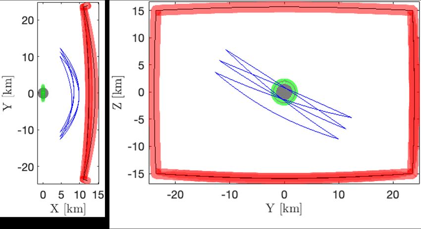
mechanization of the error was considered. The 95% confidence level for total
correction maneuver cost in the science phase is 0.069 m/s (Figure 10), while
the position error one is 2.76 km, again mainly due to uncertainty in the final
maneuver (Figure 11).
4.3.2. Release trajectory
As for the release trajectory, the approach described in Section 4.3 is exploited.
The first day after release is fully allocated to commissioning. After that, a first
OD lasting 1 day for orbit acquisition is made. This is useful to reduce the huge
dispersion given by the release. No correction maneuver is performed during the
first 7 days. Then, a second Orbit Determination is performed from day 5 and
day 6, where the deviation from the nominal path is estimated and then used
as input for the differential guidance algorithm. In the second transfer phase
leg, from the Injection Maneuver to the Science Orbit Acquisition Manuever
(SOAM), the scheme similar to the science phase one is used: two correction
maneuvers are given, the first after 4 days from the Injection Maneuver (IM)
22Figure 8: Achievable position knowledge in the science phase.
and the second after 7 days from the IM together with the SOAM. Differently
from the science loop, the first correction maneuver is not associated with any
deterministic maneuver, but it is needed in order to cope with the deviations
caused by the Injection Maneuver and to target with an increased precision the
Science Orbit Acquisition Maneuver point. In the second transfer phase leg a
cut-off time of 1.5 days is considered between the OD and the maneuvers, plus
a period of 1 day is taken into account between the maneuver and the beginning
of the OD. For the initial state uncertainty, the worst-case scenario is taken as
reference (see Section 3.3.1 for detailed discussion). Thus, a deployer release
velocity of 5 cm/s with an uncertainty of 1 cm/s (3σ) is used. The half cone
pointing error is 5 deg; on top of it the Hera pointing accuracy of 0.5 deg (3 σ)
is considered.
For clarity’s sake, the assumptions made for this analysis are summarized and
listed below:
• The guidance law is the standard differential guidance algorithm;
• Correction maneuvers are given with the IM, the SOAM and at day 4 of
the second leg;
23Figure 9: Achievable velocity knowledge in the science phase.
• No uncertainty in stochastic maneuvers is considered;
• Correction maneuvers are not applied if their value is lower than 5 mm/s;
• An initial uncertainty of 5 m on position is considered. The relative veloc-
ity with respect to Hera has a mean of 5 cm/s and a standard deviation
of 1 cm/s (3σ). A pointing error of 5 deg (3σ, half cone) with a 0.5 deg
pointing accuracy is used;
• A thrust misalignment of 1% in magnitude and 1 deg in angle (3σ) is
considered;
• The ISL is simulated taking into account an accuracy of 1 m in range and
0.1 mm/s in range-rate. The error is modeled as Gaussian noise;
• During the first leg, Orbit Acquisition is performed from day 1 to day 2,
while Orbit Determination from day 5 to day 6;
• In the second leg, a interval of 1.5 days between the maneuver and the
beginning of the OD phase is considered, while a cut-off time of 1 day is
24(a) (b)
Figure 10: (a) Navigation cost probability distribution function for science phase. On the
y-axis the number of occurrences are shown. (b) Navigation cost cumulative distribution
function for science phase.
inserted before the maneuver;
• The ISL performs a range measurement every 20 minutes and a range-rate
every 2 minutes;
• Propagation is done linearly by means of the STM, while the estimation
is done exploiting the EKF;
• 1000 samples Monte Carlo run.
Following these assumptions, a timeline for the transfer orbit can be derived.
In Figure 12, red dots indicates when the range measurements are computed,
while blue dots shows when range-rate is performed.
The knowledge analysis is reported in Figure 13 and Figure 14. They illustrate
the results of the covariance analysis and the achievable knowledge accuracy of
the spacecraft during the transfer phase. In the plots, the DidymosECLIPJ2000
reference frame is considered. The large dispersion at the beginning is only par-
tially recovered through the Orbit Determination and an error of some tens of
meters is found for the position at the SOAM. On the other hand, the veloc-
ity knowledge improves better during the transfer, leading to error less than
0.1 mm/s at the end of transfer phase. These figures show how the orbit acqui-
25(a) (b)
Figure 11: (a) Final error probability distribution function for science phase. On the y-axis
the number of occurrences are shown. (b) Final error cumulative distribution function for
science phase .
Figure 12: Transfer trajectory timeline (measurements dots are too close to be distinguished).
sition phase is beneficial to enhance the knowledge analysis in the first transfer
leg, quenching the dispersion and helping in determine the correct orbit the
spacecraft is on just after the release. The covariance analysis shows also that
the navigation costs (Figure 15) can be represented as a Gaussian distribution
of mean 0.01354 m/s and a standard deviation of 0.0039 m/s. The 95%-ile for
correction maneuver cost in the transfer phase is 2.1 cm/s.
4.4. Optical Navigaton
The baseline navigation strategy exploits information of range and range-rate
with respect to the mother spacecraft. In addition, the mission will perform an
optical navigation experiment by processing the images of the asteroids. This is
26Figure 13: Achievable position knowledge in the transfer phase
intended to validate the performances of optical navigation on-board, but will
not impact the baseline navigation strategy.
4.4.1. State-of-art methods and trade-off
Different state-of-art strategies can be adopted for optical navigation. They
range from the landmark-based methods to centroiding and disk fitting meth-
ods. The landmark navigation estimates the position of Milani based on the
natural landmarks on the asteroid surface de Santayana and Lauer (2015). It is
accurate, however is also heavy from a computational standpoint. The centroid-
ing method with disk fitting exploits the acquisition of the center of brightness
of the figure to estimate the relative line-of-sight and the external horizon to
estimate the apparent asteroid size, which is related to the relative range Gil-
Fernandez and Ortega-Hernando (2018). This method can yield a good accu-
racy, the image processing required is simple, and an accurate asteroid model
is not required. The horizon-based navigation is similar to landmark naviga-
tion, but it compares the asteroid shape and dimension as seen in the images
with an asteroid model Owen (2011). The correlation between the two yield an
27Figure 14: Achievable velocity knowledge in the transfer phase
information about the relative position and pose of Milani at a very high compu-
tational cost, and an accurate asteroid shape model is required. We performed
a trade-off analysis to select the most suitable method and the centroiding with
disk fitting resulted as the most promising one for optical navigation owing to
its accuracy, robustness, simplicity, and independency from the asteroid model
knowledge. Thus, a navigation strategy exploiting the centroiding technique
with disk fitting is baselined for navigation. During the occultation periods of
the secondary by the primary body or shadow, the navigation strategy will still
be robust, as Milani could either use ISL range and range-rate measurements or
use Didymos visual images (provided that the navigation NavCam field-of-view
will be able to image Didymos fully within the frame) or relying on on-board
propagation to avoid losing the tracking of the system. However, since the shape
of the asteroids and their features are not known, the centroiding method with
a disk fitting has been chosen as the baseline for optical navigation. In order to
assure accuracy, observability of the whole system, coverage, and efficiency of
operations, the navigation strategy uses a different navigation camera which has
28(a) (b)
Figure 15: (a) Navigation cost probability distribution function for transfer phase. On the
y-axis the number of occurrences are shown. (b) Navigation cost cumulative distribution
function for transfer phase.
a larger field-of-view and higher resolution than ASPECT. In this way, while
performing scientific operations, it is still possible to acquire navigation infor-
mation. Moreover, a separated wide-angle camera (WAC) is foreseen to grant
the full system visibility at any time. Thus, the adopted strategy for optical
navigation exploits the same target of the scientific investigation with a nav-
igation camera but keeps the observability of the two asteroids with a small
ultra-wide angle camera. In this way, the pointing is shared among science and
navigation, the navigation observables are accurate because the navigation cam-
era is dedicated to the asteroid, and the full binary system view is assured owing
to the ultra-wide angle camera. This strategy is also beneficial during the safe
mode and targets acquisition mode. The parameters of the navigation cameras
are reported in Table 5. Due to the early stage of the design process, the GNC
baseline has not been established yet in terms of hardware components. The
values in Table 5 are assumed based on typical performance of similar sensors,
and do not refer to any existing camera. A representative image of the Didy-
mos system with the three different cameras (ASPECT, NavCam, and WAC)
is shown in Figure 16.
29Table 5: Navigation camera characteristics.
Camera FOV Sensor
NavCam 21 x 16 deg 2048 x 1536 pix
WAC 40 x 40 deg 2048 x 2048 pix
Figure 16: The external frame represents the FOV of the WAC, the medium frame represents
the FOV of the NavCam, while the small asteroid is included in the small ASPECT field-of-
view. The distance at which this image is simulated is about 8.5 km from Didymos.
4.4.2. Optical Navigation Model and Methods
The image processing steps and the optical navigation method are described
in this paragraph. The image, generated according to the CubeSat trajectory,
pointing, and navcam specifications, is retrieved by Celestial Objects Rendering
Tool (CORTO), which is a tool developed at Politecnico di Milano (Figure 17,
step 1). The image is pre-processed to compute a mean background noise which
is subtracted from the image, and the image is thresholded to highlight the
bright objects in the frame (Figure 17, step 2). In this way, it is straightforward
to identify the two groups of connected pixels belonging to D1 and D2, which
can be bounded by a green box (Figure 17, step 3).
The center of brightness of each object can be easily computed by determining
the centroid of the illuminated pixels inside the green boxes (Figure 18, step 4).
The principal axes of each object can be determined, one of this axis will be
30Figure 17: Steps 1-3; Image acquisition, pre-processing, and objects detection.
Figure 18: Steps 4-6; Center of brightness (blue dot), center of mass (red dot), light direction
and lit edge estimations.
aligned with the light direction while the other in the direction orthogonal to it.
In this way, the axis of the light direction can be estimated from the images but
it can be also complemented by the sun sensor information (Figure 18, step 5).
The center of mass can be then estimated as a displacement of the center of
brightness along the negative light direction. The displacement between the
center of brightness and the center of mass is inversely proportional to the
object phase angle (Figure 18, step 5). The image is then scanned along the
light direction to identify the pixels belonging to the lit edge of each body
(Figure 18, step 6).
Owing to the estimations of both the center of mass and the lit edge of each
object in the images, a mean radius in pixels can be estimated from the center
of mass to the pixels constituting the lit edge. In this way a disk is fitted to
the object (Figure 19, step 7 for D1 and step 8 for D2). The center of mass,
the center of brightness, and the dimensions of the two objects are the outputs
that can be extracted from the image processing algorithm.
31Figure 19: Steps 7-9; D1 disk fitting and D2 disks fitting.
4.4.3. Image Processing Accuracy
The optical navigation method accuracy is evaluated by processing 150 images
randomly chosen from the nominal orbit. The procedure extracts navigation
information from the figures in a static way, thus no dynamic filtering is used
in this preliminary phase. The image processing steps extract the information
on the centroid of D1 and the apparent disk size. This information are given
in pixels and are compared to the actual ones to assess the errors involved with
the image processing. Figure 20 shows the mentioned errors, where the x and
y directions are the horizontal and vertical pixel coordinates and COM refers
to the center of mass. The error in the centroiding has a 3σ std lower than
10 pixels, while the error in the disk radius estimation has a 3σ std lower than
20 pixels.
The NavCam has a 21×16 deg FOV and a 2048×1536 pixels detector. Thus,
since every pixel spans 0.0103 deg, the worst case centroiding error is 0.103 deg.
This is equivalent to a lateral error of 12.5 m at a distance of 7 km, and a lateral
error of 17.9 m at a distance of 10 km. The worst case pixel radius error is 20
pixels (equivalent to a 0.2051 deg error). This is equivalent to a range error of
423.8 m at true distance of 7 km, and to a range error of 841.9 m at a true
distance of 10 km. Thus, the worst case range error coming from the image
processing is lower than the 10% of the true range. The error might be still
reduced by developing an on-board optical navigation filter.
32Figure 20: Center of mass error in horizontal and vertical pixel directions x and y and radius
error as output of the image processing.
4.5. Control
Milani’s nominal control architecture is expected to be based on traditional
methods. However, because of the unique operations of Milani, in concert with
other spacecraft (Hera and Juventas) and the risk of collision with either of
the asteroids, particular care is involved in the design of the Corrective Ac-
tion Maneuver (CAM) strategy. The CAM is a semi-autonomous contingency
maneuver which is executable during nominal operations, in this section the
strategy involved in the evaluation, quantification and execution of the maneu-
33Figure 21: High-level architecture of the CAM strategy.
ver is explained.
During operations Milani will be sharing the most valuable space around Didy-
mos system with Juventas and Hera. To ensure safe operations, the CubeSat
shall be capable to avoid collisions with the surrounding bodies. The safety of
Milani starts at mission analysis level with the design of trajectories that nom-
inally do not encroach with the spacecraft and asteroids. However, a high-level
strategy for the CAM is designed for unsafe deviations from nominal operations.
Its schematics is shown in Figure 21. It is desirable to avoid both collisions with
the spacecraft and with the asteroids. However, it is also important to distin-
guish between these two different events. The happening of the first one would
produce the loss of multiple systems, while the latter would involve Milani. The
collision risk can be assessed directly with the ISL range and range-rate ca-
pabilities for the spacecraft (Hera and Juventas, both active systems) while a
combination of visual images from the NavCam and ISL data can be used with
the asteroids (Didymos and Dimorphos, both passive systems).
The triggering mechanism of the CAM mode is based on the concept of risk
ranges, that are simply the estimated ranges from the spacecraft and the as-
teroids. Whenever these quantities go below a certain threshold, a correction
maneuver is considered necessary. Figure 22 shows the risk ranges associated to
Hera, Juventas and the Didymos system. Their evolution in time is describing
34Figure 22: Example of risk tubes during the science phase of Milani mission. The trajectories
of Hera (black rectangle), Juventas (inner magenta circle) and Milani (blue) are represented in
the Didymos Equatorial reference frame. The risk tubes for Hera and Juventas are represented
with radius respectively of 1 km and 500 m. A contingency spherical region of risk is assumed
for Didymos with a radius of 1.5 km.
risk tubes.
Once a corrective maneuver is requested, its orientation and magnitude are
computed. The strategy to do that on-board is based on an hybrid between a
generic and a specific look-up tables. The generic one contains only the mag-
nitude of the maneuvers as a function of the range of Milani from the colliding
object. The delta-V vector of the maneuver is directed towards the local radial
direction of Milani’s osculating orbit, opposite to the asteroid system. These
maneuvers are pre-computed on ground based on the dynamic environment of
the asteroid in such a way to ensure Milani will get further away but will not
escape the system before a certain amount of days to be specified. The specific
one contains pre-computed maneuvers both in magnitude and direction that are
evaluated with a certain timespan on the nominal trajectory. The specific one
are more accurate and can be relevant for small deviations from the nominal
trajectory, the generic one are less accurate but are designed to cover the entire
space around the colliding objects.
355. Payload operations
In this section a detailed analysis of payload operations during the scientific
phase of the mission is illustrated. In particular, we only focus on ASPECT
operations, which is the only payload that impose observational requirements
to the mission profile. The driving requirements are in terms of phase angle and
resolution. Together with resulting distances, these are summarized in Table 2
and Table 3.
A science orbit cycle of 21 days is considered in the analysis to assess the ca-
pability to fulfill the payload objective to produce global maps of the asteroids.
The time intervals within this cycle in which the constraints on the phase angle,
distance and resolution are simultaneously satisfied are considered for potential
observations.
Further pruning is performed by assessing the illumination condition and view-
ing geometry of each individual face of the asteroid shape models. Shadowing
effect of Didymos on Dimorphos are also taken into account. Considering all
these factors, it is estimated that a total cumulative time of 4.7 and 4.6 days
are available to perform scientific observations of, respectively, Didymos and
Dimorphos. There are however regions in both bodies near the south poles that
will be permanently in shadow during the mission. These cannot be observed
by ASPECT using visual imaging and are not caused by the choice of Milani
trajectories, and therefore are not accounted in the evaluation of the global
coverage.
Figure 23 and Figure 24 illustrate the faces that can be imaged during the
potential observation periods. In bot cases global coverage can be achieved
with the trajectory chosen. It is also estimated that a minimum number of
4 images timed at the proper epochs will be needed for each body to achieve
global coverage. The areas covered by them is illustrated in Figure 25 and
Figure 26.
This analysis is valid assuming ideal pointing and that the target body is entirely
within the FOV of ASPECT. If the latter case is not true, especially in the case
3690 70
Minimum angle between ASPECT and local normal [deg]
60
60
50
30
40
Phi [deg]
0
30
-30
20
-60
10
-90
-180 -135 -90 -45 0 45 90 135 180
Lambda [deg]
Figure 23: ASPECT potential global coverage on Didymos. The map represents which faces
of the shape model can be imaged by the payload given that the observation requirements are
satisfied. The color of each face represents the minimum angle between the ASPECT line of
sight and the face local normal during the science orbit cycle.
90
70
Minimum angle between ASPECT and local normal [deg]
60
60
30 50
Phi [deg]
40
0
30
-30
20
-60
10
-90
-180 -135 -90 -45 0 45 90 135 180
Lambda [deg]
Figure 24: ASPECT potential global coverage on Dimorphos. The map represents which faces
of the shape model can be imaged by the payload given that the observation requirements are
satisfied. The color of each face represents the minimum angle between the ASPECT line of
sight and the face local normal during the science orbit cycle.
3790
4
60
30
3
Image number # [-]
Phi [deg]
0
2
-30
-60
1
-90
-180 -135 -90 -45 0 45 90 135 180
Lambda [deg]
Figure 25: Simulation of an image acquisition sequence to achieve global coverage on Didymos.
The colors represent the areas of the shape model covered by each image in a sequential order.
Global coverage on the visible faces can be achieved with 4 images.
90
4
60
30
3
Image number # [-]
Phi [deg]
0
2
-30
-60
1
-90
-180 -135 -90 -45 0 45 90 135 180
Lambda [deg]
Figure 26: Simulation of an image acquisition sequence to achieve global coverage on Dimor-
phos. The colors represent the areas of the shape model covered by each image in a sequential
order. Global coverage on the visible faces can be achieved with 4 images.
38You can also read