A Pairwise SSD Fingerprinting Method of Smartphone Indoor Localization for Enhanced Usability - MDPI
←
→
Page content transcription
If your browser does not render page correctly, please read the page content below
remote sensing
Article
A Pairwise SSD Fingerprinting Method of
Smartphone Indoor Localization for
Enhanced Usability
Fan Yang 1,2 , Jian Xiong 3 , Jingbin Liu 1,4, *, Changqing Wang 2 , Zheng Li 1 and Pengfei Tong 1
and Ruizhi Chen 1,4
  1   State Key Laboratory of Information Engineering in Surveying, Mapping and Remote Sensing,
      Wuhan University, Wuhan 430079, China; fanyang1990@foxmail.com (F.Y.);
      2016206440005@whu.edu.cn (Z.L.); tongpfgiser@163.com (P.T.); ruizhi.chen@whu.edu.cn (R.C.)
 2    State Key Laboratory of Geodesy and Earth’s Geodynamics, Chinese Academy of Sciences,
      Wuhan 430079, China; whiggsdkd@asch.whigg.ac.cn
 3    Wuhan GeoTechnical Engineering and Surveying Co. Ltd., Wuhan 430079, China; tz@hbaa.cn
 4    Collaborative Innovation Center of Geospatial Technology, Wuhan University, Wuhan 430079, China
 *    Correspondence: jingbin.liu@whu.edu.cn; Tel.: +86-139-7108-2735

 Received: 18 January 2019; Accepted: 3 March 2019; Published: 8 March 2019

 Abstract: Smartphone indoor localization has attracted considerable attention over the past decade
 because of the considerable business potential in terms of indoor navigation and location-based
 services. In particular, Wi-Fi RSS (received signal strength) fingerprinting for indoor localization
 has received significant attention in the industry, for its advantage of freely using off-the-shelf
 APs (access points). However, RSS measured by heterogeneous mobile devices is generally biased
 due to the variety of embedded hardware, leading to a systematical mismatch between online
 measures and the pre-established radio maps. Additionally, the fingerprinting method based on
 a single RSS measurement usually suffers from signal fluctuations due to environmental changes
 or human body blockage, leading to possible large localization errors. In this context, this study
 proposes a space-constrained pairwise signal strength differences (PSSD) strategy to improve Wi-Fi
 fingerprinting reliability, and mitigate the effect of hardware bias of different smartphone devices on
 positioning accuracy without requiring a calibration process. With the efforts of these two aspects,
 the proposed solution enhances the usability of Wi-Fi fingerprint positioning. The PSSD approach
 consists of two critical operations in constructing particular fingerprints. First, we construct the signal
 strength difference (SSD) radio map of the area of interest, which uses the RSS differences between
 APs to minimize the device-dependent effect. Then, the pairwise RSS fingerprints are constructed by
 leveraging the time-series RSS measurements and potential spatial topology of pedestrian locations
 of these measurement epochs, and consequently reducing possible large positioning errors. To verify
 the proposed PSSD method, we carry out extensive experiments with various Android smartphones
 in a campus building. In the case of heterogeneous devices, the experimental results demonstrate
 that PSSD fingerprinting achieves a mean error ∼20% less than conventional RSS fingerprinting.
 In addition, PSSD fingerprinting achieves a 90-percentile accuracy of no greater than 5.5 m across the
 tested heterogeneous smartphones

 Keywords: indoor localization; smartphone navigation; received signal strength (RSS); pedestrian
 dead reckoning (PDR)

Remote Sens. 2019, 11, 566; doi:10.3390/rs11050566                      www.mdpi.com/journal/remotesensing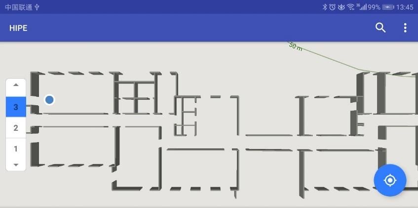
Remote Sens. 2019, 11, 566                                                                            2 of 24

1. Introduction
     Because of the popularity of built-in global navigation satellite systems (GNSSs) with smartphones,
smartphone navigation has been one of the most popular applications. Smartphone navigation not
only facilitates daily mobility by providing routing navigation from place A to place B; it also becomes
a major data source for big data analysis in urban intelligent transportation. However, GNSS does not
work in indoor spaces, where indoor navigation and location-based services (LBS) have considerably
more business potential than current GNSS navigation outdoors [1–3]. Therefore, smartphone indoor
localization has attracted considerable study efforts in the past decade to provide a smartphone with the
capability of indoor localization, and a variety of solutions have been presented in the literature [4–6].
Signals of opportunity-based solutions, such as Wi-Fi fingerprinting, have been studied largely in the
context of smartphone applications because of the advantages of low cost and the requirement of no
additional infrastructure. Unfortunately, few of these reported solutions have been applied widely in
real marketing due to several issues regarding the usability. These studies focused on the localization
accuracy, while the usability was neglected. For smartphone mass users, usability is important for user
experience and applicability of the solution, and therefore, usability must be considered in particular
in the algorithm design.
     Previous work has proposed many approaches to realize Wi-Fi indoor localization, of which
fingerprinting based on received signal strength (RSS) has attracted the most attention because
no prior knowledge of infrastructure position is needed compared to the traditional geometric
methods [7]. Moreover, the high requirement of hardware ensuring precise ranging and a particular
radio attenuation model specified for the indoor environment make the geometric method less
applicable [8]. The philosophy behind the RSS-based fingerprinting approach is to first collect
fingerprints in terms of RSS signatures labeled with the corresponding coordinates at a database
for the offline training phase. Then, for the online phase, the user’s location can be determined
with the best-fitted fingerprint by comparing the measured RSS against the prebuilt database [9].
When only Wi-Fi is considered to be the location source, past work reports that either deterministic
algorithms such as K-nearest neighbor (KNN) [10] or the probability (Bayesian) algorithm [9,11] in
terms of RSS fingerprint expects to locate the user/device at a precision of approximately 5 m for many
instances [12]. However, the following challenges remain in terms of usability:
•     The heterogeneity of devices. For most of the cases, the assumption of the RSS fingerprinting
      method is that the devices collecting RSSI for both the offline training phase and the online phase
      are identical or homogeneous; otherwise, the localization accuracy is significantly degraded.
      This is because the RSS is influenced by a particular transmitter-receiver pair’s hardware-specific
      parameters, such as antenna gains [13]. To overcome this, Haeberlen [14] and Kjærgaard [15]
      proposed a precalibration method to translate the RSS of heterogeneous devices into the
      benchmark device by a set of conversion formulae. However, the formulae must be found
      and validated in the lab in advance, which is impractical and time-consuming with the increasing
      number of new mobile devices. Therefore, developing a free-calibration method to reduce
      effects caused by heterogeneous mobile devices is a challenge towards the goal of ∼5 m
      location precision.
•     The reliability of positioning. This great challenge is the result of the large errors in
      RSS fingerprinting localization due to the signal fluctuations caused by many factors, i.e.,
      the time-varying environments or body blockages [16]. The large errors usually manifest as
      a large gap between current Wi-Fi prediction and the previous prediction, which is apparently
      unreasonable because a pedestrian’s historic walk track should be continuous. Some of the past
      works attempted to reduce the signal fluctuations regarding one or two aspects [17], but currently,
      there is no single universal solution for all cases. In addition, another direction is to leverage the
      relatively stable external sources in a fusion frame, typically, the PDR (pedestrian dead reckoning)
      derived information including the pedestrian’s heading and walking distance [18,19]. With a
      deliberately designed filter, the fusion can smooth the sequence of Wi-Fi positioning and minimize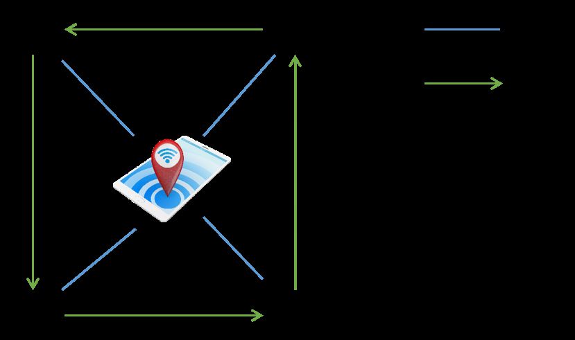
Remote Sens. 2019, 11, 566                                                                           3 of 24

      the large errors. However, frequent erroneous Wi-Fi positioning will undermine the filtering.
      Hence, it is still necessary to enhance the reliability of Wi-Fi positioning. How to design a pure
      Wi-Fi positioning system by increasing the diversity of fingerprints to further reduce large errors
      is a considerable challenge.

     The error sources such as device differences and body blockages as well as temporal environmental
changes, can be hardly avoided when fingerprinting approach is applied in reality. Rather than
particular treatments with the error sources one by one, this study attempts to tolerate the errors
by imposing additional spatial constrains directly in the fingerprints for the first time. To this end,
we propose a pairwise signal strength difference (PSSD) indoor location system, which is extended
from the traditional Wi-Fi-RSS fingerprinting method. The basic rational behind PSSD arises from two
aspects regarding the two challenges depicted. The first aspect is that the signal strength difference
(SSD) that differentiates the RSS between APs is more stable than an absolute RSS value; and more
importantly, the SSD is mathematically feasible for heterogeneous mobile devices. Another aspect
is an introduction of spatial constrain into fingerprints by using a pairwise RSS observations to
predict the pedestrian’s walk track. Compared to the conventional RSS point-value positioning
system, the pairwise fingerprint with user’s movement information should be more robust and be less
interrupted by those unavoidable error sources. Therefore, unlike several existing Wi-Fi fingerprinting
approaches, the proposed PSSD actually establishes two types of fingerprint databases, SSD and
pairwise RSS radio maps. In this way, our system can deal with diverse RSS measurements from
heterogeneous devices and possible large errors between Wi-Fi predictions.
     The paper is organized as follows. We first review the related work in Section 2. Subsequently,
Section 3 details the proposed method from three aspects, the conventional SSD algorithm as well as
our modification, the spatial information extraction, and finally the pairwise RSS method. In Section 4,
we present and discuss the experimental results of the proposed PSSD method. Finally, we draw
conclusions in Section 5 and propose future work.

2. Related Work
     Wi-Fi RSS fingerprinting-based localization has been extensively studied over the past decade.
Here, we only focus on the related work concerning the above two challenges.
     As mentioned before, the heterogeneity of devices can significantly degrade the positioning
performance of RSS-based fingerprinting. Therefore, past work proposed a manual adjustment of
RSS signals to reduce positional error [14,15], which is not scalable as the number of new devices
increases. In this respect, some works such as Tsui et al. [20] reduced the training time between devices
to realize faster precalibration. Nevertheless, training for all brands of smartphones is still impractical
because of the time and money cost. Therefore, free-calibration methods have drawn considerable
attention recently. A typical free-calibration method uses similarity metrics at the online match phase
instead of conventional distance metrics, i.e., Euclidean distance. The similarity metrics such as
cosine/Pearson/Spearman similarity have been heavily addressed in past works [14,21–23]. However,
the stability of this method remains a challenge because of its assumption that the RSS differences
caused by hardware is constant; however, the differences are unknown. Moreover, this approach is
mathematically less reliable if the dimensions of the calculated vectors are insufficient [8].
     Another type of free-calibration method is the RSS difference method, and the basic rational
behind this method is the differential of the RSSs between APs or between positions, can minimize
the effects created by heterogeneous devices. For example, as the user is walking towards an AP,
he will obtain increasing RSS measurements with high probability, regardless of the AP’s absolute
transmission power and the model of the sensing device [8]; this is called the RSS gradient, which
is basically a differential RSSs between positions. In contrast, the other RSS difference methods,
including the SSD [13], DIFF [24] and MDF [25], leverage the RSS difference between APs. In particular,
the SSD approach draws the most attention; Liu et al. [26] and Kjrgaard and Munk [27] developed a
hyperbolic positioning algorithm based on the distance differences that are converted from SSDs and
Remote Sens. 2019, 11, 566 4 of 24
minimized the positional errors. Unlike the geometric SSD approach, Hossain et al. [13] proposed a
location fingerprint with SSD and demonstrated that it outperforms the traditional RSS fingerprint
analytically and experimentally. Nevertheless, the SSD fingerprint amplifies the noise level and loses
the discriminative information, leading to a potential reduction in accuracy compared to the raw
RSS fingerprint with homogenous devices [28,29]. In this study, our PSSD system modifies the SSD
fingerprint to make it more robust, and leverages the similarity metric to optimize the localization
as well.
The RSS variation is another key factor towards accurate Wi-Fi positioning systems. However,
the RSS observable is susceptible to the phenomena of interference, jumping, and instability, which
are caused for many [8] such as the time-varying environments, human body blockage, and other
unpredictable outliers. From the authors’ point of view, there are two types of solutions to mitigate the
large positional errors caused by RSS random variation. The first solution departs from the perspective
of RSS variation and its cause. For instance, Wu et al. [16] uncovered outdated RSS in real-time
measurements and developed a robust regression to tolerate this type of outlier. Fet et al. [30] suggested
collecting orientation-dependent fingerprints for multiple directions to reduce the errors created by
human blockage. Haeberlen [14] proposed a linear RSS transformation formula to compensate for
environmental change, etc. However, these methods usually require considerable labor while offering
minor improvement [16] and none of these methods has considered all aspects of the causes of
RSS variation.
Another solution for mitigating the large error is the fusion with additional localization sources
through Kalman filtering or particle filtering [31,32]. In a typical scenario of ubiquitous localization,
the PDR is usually the primary option for fusing Wi-Fi because of its accurate positioning in a short time.
Intensive experiments on PDR/Wi-Fi fusion have been conducted, and found a significant positioning
precision improvement [33–35]. Despite the improvements, unstable human locomotion while walking
and accumulated errors in inertial sensing make single-state PDR inapplicable for all states [36,37].
Therefore, fusion of Wi-Fi and single-state PDR in terms of the absolute walk heading/distance per step
is not universal. Based on the previous work, our PSSD approach does not adopt the fusion scheme but
directly increases the diversity of fingerprints to realize error mitigation, and in this sense, it is more
similar to the first solution. Nevertheless, the diversity gain of fingerprints in PSSD comes from the
spatial constraints offered by the range estimation of PDR’s heading/distance within two Wi-Fi scans.
Compared to the absolute heading/distance estimation, the range estimation of heading/distance
is only raw information, but it becomes more reliable. In summary, the proposed PSSD exploits the
reliable PDR information in terms of the fingerprinting level instead of the positioning level and this
kind of method has never been addressed before to the best of our knowledge.
3. Method
The proposed PSSD approach enhances the usability of Wi-Fi positioning through leveraging
three features: the SSD radio map, the spatial information extracted from PDR, and the pairwise RSS
radio map.
In the offline training phase, a radio map called PSSD is constructed. The PSSD contains two
layers: the first layer is based on the SSD approach to mitigate the hardware differences between
smartphones, and the second layer is based on the pairwise RSS approach that exploits the geometric
relation between reference points. Thus, we clarify the combination of these two radio maps in that
(1) the SSD approach slightly lowers the location accuracy compared to the traditional RSS, thus
SSD is only used to determine a series of candidate positioning points rather than the ultimate point,
(2) the pairwise RSS approach is designed for minimizing large location errors at the price of a higher
computational load than the normal method, and thus, selection of the best-fitting point from the
candidates in previous step rather than the whole radio map can largely reduce the computational cost.
During the positioning inference phase, the RSS observables are first transformed into the SSD
format to pick up five candidate match points from the prebuild SSD radio map. Subsequently,Remote Sens. 2019, 11, 566 5 of 24
the spatial information inferred by the step detection and heading estimation from PDR are extracted.
In addition, the RSS measurements are transformed into a pairwise format, which is marked with the
spatial information extracted in the previous step. Thus, the final best-fitting positioning point can
be determined from the previous five candidates through the pairwise RSS radio map. The overall
working flowchart of the proposed PSSD is shown in Figure 1. We will detail each module in the
following subsections.
WiFi RSS data Sensor data
Offline RSS training Mobility
phase recognition
SSD Radio Online Location Raw direction
Maps (Euclidean distance) sensing
Pair-wise Online Location
RSS Radio
(Pearson Similarity)
Maps
Location-based service and applications
Figure 1. Overall working flowchart for proposed Pairwise Signal Strength Difference (PSSD) approach.
3.1. SSD Radio Map Construction and Online Inference
Generally, the samples’ RSS values collected over a small time window are averaged to constitute
the radio map in the offline phase for a deterministic KNN method [38]. However, having a different
device in the online positioning phase would likely lead to a systematic bias of the RSS signature at the
same location, and consequently lead to a mismatch with the already-built radio map. This can refer to
the log-normal shadowing model for the traditional RF transmitter-receiver pair, as below [39]:
d
P(d)|dBm − P(d0 )|dBm = −10β log( ) + XdB (1)
d0
where P(d) denotes the RSS at an arbitrary distance d from the transmitter, and d0 denotes the
reference distance such as 1 m. The β on the right side of Equation (1) denotes the mass loss exponents,
while the second term XdB reflects the signal variation that is subject to the Gaussian distribution
2 )). It should be noted that the perceived power P ( d ) at the reference point depends
( XdB ∼ N (0, σdB 0
on the device collecting the data, evidenced by the free space propagation model [40] as shown below,
PAPi G APi Gdevice λ2AP
i
P(d0 )|dBm = 10 log( ) (2)
16π 2 d20 LRemote Sens. 2019, 11, 566 6 of 24
where PAPi is the ith AP’s transmitted power, G APi is the ith AP’s antenna gain, Gdevice is the
end-device’s antenna gain, L is the system loss factor, and λ APi is the transmitting carrier’s wavelength.
It is apparent that the term Gdevice makes the RSS measurement relevant to the device. Rather than
using absolute RSS values as location fingerprints, we show that the difference in the RSS values
observed by two APs (i.e., SSD) can be used to define a more robust signature for a transmitting mobile
device; see a simple demo in Figure 2. With Equations (1) and (2), we directly present the mathematical
form of SSD (denoted as δ) for the ith and jth APs without any deduction as follows:
AP APj
δAPi,j |dB = P(di )|dBmi − P(d j )|dBm
PAPi G APi λ2AP L j di dj (3)
i
=10 log( ) − 10β i log( ) + 10β j log( ) + [ Xi − X j ]dB .
PAPj G APj λ2AP Li d0 d0
j
More details about the formulation of Equation (3) can be found in Hossain et al. [13]. As we can
see in Equation (3), SSD contains no device-relevant parameters (i.e., Gdevice ) when compared to the
absolute RSS shown in Equation (2), and consequently does not suffer from the device-different effect
in theory. To support this, we conduct an experiment at three arbitrary training positions using three
brands of mobile phones, see Figure 3.
Figure 2. The usage of RSS and SSD from multiple APs.
The left panel of Figure 3 denotes the conventional RSSs measured by smartphones where it can
be seen that the differences between the RSS curves can constantly reach up to 15 dB, which might be
intolerant for RSS fingerprinting system. Instead, the SSD depicted by the right panel of Figure 3 has
manifested a better consistency between mobile phones. Therefore, when not considering the noise
level, the SSD fingerprint should be more desirable for heterogeneous devices. However, according to
the error propagation law, SSD has a √ lower signal-to-noise level than RSS due to the term [ Xi − X j ]dB
that amplifies the noise variance to 2σdB . This side effect is unavoidable and slightly affects the
localization accuracy that will be shown later in an experiment. Apart from this point, we also note
that the freedom of SSD observations is less than that of RSS. For instance, at the ith round of the Wi-Fi
scan, we obtain the RSS observations Fi as follows:
Fi = [S1 , S2 , ...Sn , ...S N −1 , S N ], (4)
where Sn denotes the RSS of the nth AP. In addition, after converting the RSS to SSD by Equation (3),
we find:
0 S1 − S2 S1 − S3 ... S1 − Sn ... S1 − S N
0 S2 − S3 ... S2 − Sn ... S2 − S N
0 ... ... ... ...
Di = 0 Sm − Sn ... Sm − S N (5)
0 ... ...
0 S N −1 − S N
0Remote Sens. 2019, 11, 566 7 of 24
RSS variation SSD variation
60 SamSung-S8
D10
E
55 Honor 8
|RSSI| for RP 0
HuaWei P10
50 0
45
10
40
12 13 14 15 16 17 18 19 20 13 14 15 16 17 18 19 20
60
F10
G
|RSSI| for RP 1
50
0
40
10
30
12 13 14 15 16 17 18 19 20 13 14 15 16 17 18 19 20
60
H10
I
|RSSI| for RP 2
50 0
10
40
12 13 14 15 16 17 18 19 20 13 14 15 16 17 18 19 20
AP No. AP No.
Figure 3. RSS versus SSD on three arbitrary reference points (RPs) collected by a Samsung-S8, Honor 8
and Huawei P10. (a,b) are performed on RP No. 0, (c,d) are performed on RP No. 1, and (e,f) are
performed on RP No. 2.
A direct use of Equation (5) may lead to a high computational burden due to the high dimensions,
so that a simplification of Equation (5) is necessary. It is apparent that the matrix form of SSD denoted
by Di is highly correlated, and the freedom of Di is only N − 1 if we extract the maximal linearly
independent group to present Di as below:
Di = [S1 − S2 , S2 − S3 , ...Sn − Sn+1 , ..., S N −2 − S N −1 , S N −1 − S N ], (6)
Previous literature usually implemented the SSD algorithm according to Equation (6) without
more consideration. Here, we note that many previous studies prefer to carry out experiments in
an environment that researchers are familiar with. For instance, they normally distribute the APs at
specified locations as uniformly as possible in advance and ensure that the APs are strong enough to
cover almost all the experimental environment. However, this is inconsistent with reality, because you
can never have knowledge of the precise location and the coverage of each AP at a shopping mall that
you have never accessed before.
Therefore, a potential risk of Equation (6) would arise in practice when you have no predeployed
APs. Assuming that the S2 is not accessible for one round of Wi-Fi scan, SSD Di will, therefore, lose
two dimensions (S1 − S2 and S2 − S3 ) while the RSS vector Fi will only lose one dimension, as follows:
missing
z}|{
Fi = [S1 , S2 , ...Sn , ...S N −1 , S N ],
(7)
Di = [S1 − S2 , S2 − S3 , ...Sn − Sn+1 , ..., S N −2 − S N −1 , S N −1 − S N ],
| {z }
missingRemote Sens. 2019, 11, 566 8 of 24
Assuming that the number of missing APs is L, then the valid dimensions of RSS and SSD are
N − L and N − 2L, respectively. In addition, the occurrence of missing APs occurs quite often in
practical Wi-Fi scans. Here, we conduct a test and summarize the results in Figure 4, from which it can
be seen that the Samsung captured 42 APs at least and 58 APs at most. However, Mix2 captures 28∼45
APs. Not mentioning the heterogeneous devices, this experiment tells us that some APs would be
frequently missing during a Wi-Fi scan even for the same device. Obviously, the traditional SSD shown
by Equation (6) is not robust for this case, and thus, we attempt to modify Equation (5) to strengthen
the stability of the SSD. Considering Equation (5), we extract another linearly independent group as
complementary to Equation (6), and thus formulates the ultimate form of our SSD as shown below,
Di = [S1 − S2 , S2 − S3 , ...Sn − Sn+1 , ..., S N −2 − S N −1 , S N −1 − S N ,
(8)
S1 − S3 , S2 − S4 , ...Sn−1 − Sn+1 , ..., S N −3 − S N −1 , S N −2 − S N , S N −1 − S1 ],
70
Mix2 SamSung
Received number of APs
60
50
40
30
20
10
0
1 2 3 4 5 6 7 8 9 10 11 12 13 14 15
Round No. of the WiFi scans
Figure 4. Number of APs detected for each round of Wi-Fi scans in terms of Mix2 and the Samsung S8.
Here, 15 rounds of scans are summarized, and it is noted that Mix2 is a brand of smartphone produced
by Xiaomi in China.
According to Equation (7), the dimensions of SSD increase to 2N − 3. Thus, the missing AP3 only
causes the valid dimension (linearly independent) of SSD to decrease by 1 rather than 2. In addition,
we believe that our SSD could better deal with the heterogeneous device problem than the previous
SSD approach, and the only price is the additional computational load due to the increasing dimensions.
Thus, for both the online and offline stages, the original RSS must be reformatted to the SSD as the
pseudo-observations and the radio maps. Subsequently, the normal KNN with K = 5 and Euler
distance metrics are applied to select the five best-fitted candidates from the dataset. However, unlike
the previous works that tend to average the K candidates, we transfer these candidates to the next step
to have a further selection, and therefore, a relatively large K such as K = 5 is empirically preferred.
We note that the term “SSD” in the following denotes our modified SSD instead of the previous original
SSD if there are no particular statements.
3.2. Spatial Mobility Information Extraction
The nature of the pairwise RSS approach is based on the fact that the user can only move within a
limited distance between two Wi-Fi RSS scans. The pairwise RSS maps can be labeled with the spatial
geometric information beforehand and further optimize the online inference procedure with the user’s
mobility information. Before extracting the pedestrian’s mobility information, there are three questions
that need to be answered. (1) How long is the time period between RSS scans? (2) How far can the
pedestrian walk during the period? (3) What is the pedestrian’s heading during the period. These
questions are key for constraining the search in the radio map. Figure 5 shows the possible range of aRemote Sens. 2019, 11, 566 9 of 24
pedestrian’s walk distance/heading in different modes between Wi-Fi scans, and this raw information
is coupled with the spatial topological relations between reference points.
Normal Walking Keep static Fast Walking
Time Line
RSS RSS RSS RSS
Walking
range
Figure 5. An example of a pedestrian’s possible walking status while constantly receiving the Wi-Fi
RSS scans. Here, the walking speeds are classified into fast, static and normal modes, and each of the
speeds corresponds to a predefined walk range denoted as the gray solid circle. Meanwhile, the range
of the pedestrian’s walk direction between RSS scans is recorded and denoted as the blue sectors.
To answer the first question, we conduct an investigation of the average scan time between
two valid RSSs (excluding invalid scans such as the repeated scans), on the most popular brands of
smartphones (with Android platform only) in our daily life. We find that the valid RSS scan period for
most smartphones is at [1.5, 2.5] seconds after 100 scans for each phone. Actually, most smartphones at
normal working status require at least 1.2 s to finish one round of Wi-Fi scanning because an access
point broadcasts a beacon approximately every 100 ms so that in theory, the device requires at least
1.2 s across the 12 frequency channels to scan all the access points.
To question two, step frequency in indoor environments ranges primarily from 1 Hz (slow walk)
to 3 Hz (walking briskly or running) [41], and it is approximately 1.5 Hz in normal mode. To verify
this, a step detection framework has been designed as follows. Due to the physiological characteristics
of the pedestrian, the waveform of the accelerometer values (norm of the three-axis values) contains
some particular cyclical characteristics and thus can be used to detect the step update. According to
the characteristic, our system framework comprehensively includes three techniques. (1) A moving
averaging window of length 15 to filter the high-frequency noise at the ith accelerometer raw data
Accraw
i , see Figure 6 left panel. (2) A peak detection to prevent small jitters by applying a threshold of
peak value (Acc peak ) and interval (∆T) between every two adjacent peaks, see Figure 6 right panel. (3)
A zero-cross detection with adjacent accelerometer measures to find the step end, see Figure 6 right
panel. In summary, a valid step should satisfy the following,
q
Accraw
i = a2x + a2y + a2z − g
smooth = ( j=i
∑ j=i−14 Accraw
Acci j ) /15
Acc peak > Acc Threshold (9)
∆T > ∆TThreshold
Accsmooth > 0, Accsmooth < 0
i −1 iRemote Sens. 2019, 11, 566 10 of 24
where the a x , ay , az denote the three-axis accelerometer values and g denotes the local gravity
acceleration. Herein the Acc Threshold is taken as 0.7 m/s2 , and ∆TThreshold is taken as 260 ms in our
experiment given that the pedestrian is carrying the phone in “typing” mode. Another experiment is
conducted to validate our step detection scheme, see Figure 7. The detected steps (in green circles)
amount to 67, which is the same as the ground truth. In particular, a deeper insight into Figure 7
shows that the 67 steps occurred during 40 s, and this supports that the pedestrian’s step frequency
is approximately 1.5 Hz. Assuming that the stride length is approximately 0.6∼0.8 m, then we can
infer that the normal walking speed is approximately 1∼1.2 m/s, and thus, the pedestrian can walk
a distance of 3 m between two RSS scans in the period of [1.5, 2.5] s. Similarly, the pedestrian in a
fast mode will walk a distance of 6 m between two RSS scans. The recognition of normal mode and
fast mode can be realized by the step detection strategy or machine learning, yet the discussion is
obviously beyond the scope of this paper.
A low-pass filter Peak detection + Zero-cross detection
14 1.5
∆T Valid peak
12 Peak
1
10
Acceleration [m/s2]
Acceleration [m/s ]
2
0.5 False Peak
8
6 0
Moving window
4 Step end Step end
Raw Acc -0.5
Smoothed Acc
2
Smoothed Acc
-1 Peak Threshold
0
Zero-cross detection
-2 -1.5
10 10.5 11 11.5 12 12.5 13 43.5 44 44.5 45 45.5
Time [s] Time [s]
Figure 6. The left panel denotes the low-pass filtering method by a moving averaging window, and the
right panel shows the peak selection and the determination of step end. The occurrence of a valid peak
and step end within one cycle will account for one step.
3
2
Acceleration [m/s2]
1
0
-1
-2
0 5 10 15 20 25 30 35 40 45 50
Time [s]
Figure 7. An experiment of a pedestrian walking at the normal status (ground truth is 67, and the
detected step count is also 67). The green circle represents the detected steps, and the subsequent black
dashed line denotes the finish time of this step.
Let us consider question three; that is, what is the pedestrian’s heading range during the
period? First, we know the yaw of the pedestrian can be estimated from the acceleration sensor,
magnetic sensor, and gyroscope sensor. The fusion of these sensors is performed through the
quaternions complementary filter. Quaternions offer an angle-axis solution to rotations which do not
suffer from many of the singularities, including gimbal lock, that are found with rotation matrices.Remote Sens. 2019, 11, 566 11 of 24
A complementary filter is used to fuse the two orientation estimations (the gyroscope θ gyro and
acceleration/magnetic θ acc/mag ) together in the frequency domain, as below,
Z
θ f usion = α θ̇ gyro dt + (1 − α)θ acc/mag , (10)
In above equation, α is defined as α = timeConstant/(timeConstant + dt), where the timeConstant
is the length of the signals the filter should act on, and dt is the sample period (1/frequency) of the
sensor. The implementation of this algorithm is performed by publicly available software, namely,
Fsensor provided by https://github.com/KalebKE/FSensor. A static test on this algorithm shows
the standard deviation is within 3 degrees. However, considering the environmental disturbance
from both the pedestrian and magnetic abnormity, we empirically set the uncertainty (3 times of the
t
standard deviation) to 10 degrees. Thus, a series of heading angles Atii−1 can be acquired between any
t
two moments (ti , ti−1 ), and furthermore, the range Rtii−1 of the pedestrian’s walk between two Wi-Fi
scans can be derived by
t [
Atii−1 = θ f usion
t t t
(11)
Rtii−1 = [min( Atii−1 ) − 10, max( Atii−1 ) + 10]
In summary, in static mode, the user’s walk range is less than a minor quantity such as 0.1 m,
see Figure 5; in fast/normal mode, the range changes to 6 m and 3 m, respectively, manifested as the
radius of the circles in Figure 5. Moreover, the heading range is also restricted within the blue sectors
in Figure 5. This information constructs the spatial constraint that will be used later.
3.3. Pairwise RSS Radio Map Construction and Online Inference
Unlike the traditional radio map that uses the form of point distribution, the pairwise RSS map
creates a vector-based format leveraging the spatial geometric information between reference points.
Traditional RSS map construction is based on the RSS collection that requires the user to remain
stationary, but this type of radio map is obviously inconsistent with the reality. The user’s location
is indeed moving but not fixed at the discrete points/nodes, and the RSS is also collected along the
walking route but is not fixed at a certain time epoch. Thus, our work relates each node’s RSS with its
neighborhood, and in this way, reshapes the point-based RSS to a pairwise RSS.
Assuming that δ denotes the Euclidean distance between two nodes, then the set of neighborhoods
of a given node a in the radius δ∗ can be derived as
U ( a, δ∗ ) = x | a − x | < δ∗ .
(12)
where the δ∗ is optional, such as 3 or 6 m. The traditional fingerprint at node a is denoted Fa
(see, Equation (4)), and we thus define the pairwise fingerprint Pa,b for the center node a and its
neighbor node b as below,
Pa,b = [ Fa , Fb ] = [S1a , S2a , ...Sna , ...S aN −1 , S aN , S1b , S2b , ...Snb , ...SbN −1 , SbN ], ∀b ∈ U ( a, δ∗ ) (13)
In addition to the added distance information, the new “vector” form of fingerprint can record the
direction information as well. Given the coordinates of node a and b in the plane rectangular coordinate
system, we derive the azimuth of a with respect to b as θ = arccos( ~a·~b ), which is appended to Pa,b
|~a|×|~b| θ
as a label. If the traditional point-distributed RSS radio map has m reference points, as node a moves
until the whole map is covered, a completely new fingerprint database, whose number of “reference
points” should be subject to aa= ∗
S m
=1 U ( a, δ ) is created. It should be noted that the reference point in
terms of its original form denotes the a or b that is actually a true point in the physical world, but herein
the “reference point” induced from Equation (13) is simply a mathematical conception (a pair form of
true points ( a, b)) and has no physical content. Consequently, the best-fitting positioning point selectedRemote Sens. 2019, 11, 566 12 of 24
from our radio map is the form ( a, b) rather than a or b. However, there is a convention or mapping ζ
defined by us between the vector result and the physical location; that is
ζ : ( x, b) −→ b, ∀ x ∈ U (b, δ∗ ) (14)
where x denotes an arbitrary point distributed within the neighbor of point b, which means the
pedestrian’s position referred by ( x, b) is indeed the position of point b.
Apparently, the dimension or the number of “reference points” derived from aa= ∗
S m
=1 U ( a, δ ) has
greatly exceeded the original number m of the true reference points, and it continues to increase as δ∗
increases. Within expectation, the computational load of online inference in terms of this very large
database (too large δ∗ ) will be intolerant. To prevent the very large database problem that may lead to
the infeasibility of KNN, we decrease the neighborhood range according to our experience from the
previous subsection, which means δ∗ is only set to 3 m and 6 m (see Figure 8). Moreover, we restrict
the number of candidate reference points (m = 5) offered by the SSD approach, and by combining
with the heading information, the dimensions of the real-time fingerprint database are significantly
reduced, which will be demonstrated later.
North
Still
Fast
3
Normal
2m
2m
East
Figure 8. An example of the construction of a pairwise RSS fingerprint database associated with the
topological information. Three types of topological information are demonstrated for the still, fast,
and normal modes. Please note that we set the grid length to an average of 2 m in accordance with the
general performance of fingerprinting-based positioning methods.
In the online phase, the current ith RSS measurements Fi must be transformed as well to remain in
accordance with the pairwise RSS fingerprint database. Hence, the current RSS and the previous RSS
are combined into a new measurement Mi−1,i as shown below:
Mi−1,i = [ Fi−1 , Fi ] = [S1i−1 , S2i−1 , ...Sni−1 , ...SiN−−1 1 , SiN−1 , S1i , S2i , ...Sni , ...SiN −1 , SiN ], (15)
In addition, the current walking status between two RSS scans, recognized by the step detection
algorithm or machine learning, is recorded as well, including three major modes: still, fast, and normal.
The classified three modes correspond to three different fingerprint databases aa= ∗
S m
=1 U ( a, δ ). In more
∗ ∗ ∗
details, δ = 0.1 for the “still” mode, δ = 3 for the “normal” mode, and δ = 6 for the “fast”
t
mode. Simultaneously, the heading range Rtii−1 of the pedestrian is recorded as well, according to
Equation (11). The walking speed and heading range are the pedestrian’s mobility information that
will determine the pedestrian’s relative positions between RSS scans.
Subsequently, unlike the previous work that establishes a radio map and keeps it constant in
online inference phase to locate the optimal position point, our radio map or the fingerprint database
is only one subset of the whole database and it adaptively changes continuously according to theRemote Sens. 2019, 11, 566 13 of 24
varying spatial information induced by the pedestrian’s mobility. Every time the RSS (Fi ) is updated,
we retrieve a subset of the radio map (named after Pmap, and Pmap ⊆ aa= ∗
S m
=1 U ( a, δ )) as shown below:
t
Pmapi = { P( a, b) θ ∈ Rtii−1 , δ∗ ∈ {0.1, 3, 6}, b ∈ C } (16)
where C is the union of five candidate positioning points from the SSD approach, and θ is the angle
information for vector ( a, b) that was previously derived. Thus, there is a one-to-one corresponding
(measurement Mi−1,i , database Pmapi ) map that is built simultaneously. In addition, the online match
algorithm adopts the KNN with the distance metric of Pearson similarity. Considering two groups of
measurements such as A = ( A1 , A2 , ..., An ) and B = ( B1 , B2 , ..., Bn ), the similarity between these two
vectors in terms of the Pearson coefficient is,
∑1n (( Ai − A) × ( Bi − B))
S( A, B) = q q (17)
∑1n ( Ai − A)2 × ∑1n ( Bi − B)2
Use of similarity as the distance metric within the KNN algorithm has the advantage on
minimizing device differences, which was discussed in the introduction. In addition, the dimension
increase of Pa,b with respect to Fb makes the similarity metric more reliable. Finally, we summarize the
online match procedures (shown by Equation (18) as well as Figure 9) that (1) the RSS map in terms
of reference points are transformed into pairwise fingerprints beforehand, (2) in the online inference
phase, the previous RSS measurement and the current measurement are grouped and reformatted
to the pairwise form, (3) subsequently the spatial information including the walking speed and
heading range are derived to select a subset Pmap from the whole fingerprint database, and (4) finally,
the new pairwise measurement is compared to Pmap and to locate the user’s position with the Pearson
similarity metric. Please find all the procedures in Figure 9.
arg maxx (S( Mi−1,i , x ), ∀ x ∈ Pmapi ) =⇒ xSmax =⇒ ( a, b) =⇒ b (18)
Whole fingerprinting
Fast
RP map
Normal
Pmap Positioning
point
Still Normal
Measurements Spatial Information
RSSIi-1 RSSIi Reformation Extraction
Figure 9. The generation of the Pmap in terms of “vector” form from the classical RSS radio map in
terms of the reference point (RP), and the online inference procedure with the Pmap and the reformatted
measurements leveraging real-time mobility information.
4. Experiments and Results
In this positioning experiment, the mean error, root-mean-square (RMS) error, and the 95% error in
the positioning results of the three fingerprinting algorithms are compared in different actual scenarios.
The objective of the experiments is to compare the positioning performance of the proposed PSSD
algorithm with that of two legacy algorithms, SSD and RSS fingerprints. It should be noted thatRemote Sens. 2019, 11, 566 14 of 24
all these fingerprinting algorithms are based on the deterministic method (KNN) to locate the final
positioning point.
4.1. Static Test for SSD Method
As mentioned in previous, the traditional SSD theoretically suffers from dimension loss because
of missing APs, see Equation (6). In this context, we propose a modification of SSD (namely, MSSD) to
mitigate the dimension loss effect, see Equation (8). Here, we conduct a test at a static environment
to compare these two methods. An empty hall of our laboratory was selected as the test field,
where 20 reference points (numbered from 0 to 19) are distributed uniformly on the floor with an
interval of about 2 m (horizontal 2.2 m and vertical 1.8 m), see Figure 10a. The Samsung S8 was
chosen to establish the fingerprints. In the offline training phase, we collect the RSS information at
each reference point for 30 rounds, and finally average the 30 times of scans to establish the traditional
RSS fingerprint according to Equation (4). In the online phase, the user was asked for standing still at
each reference point to collect 15 rounds of RSS with Samsung S8 and XiaoMi, respectively. Therefore,
the ground truth is easily recorded and 300 groups of measurements for each smartphone in total are
evaluated to compare the SSD and MSSD approaches. It should be noted that to isolate the errors
caused by varying environments and the body blockage, the user was asked for keeping the same
gesture and direction at online and offline phases, moreover the online measurements were collected
soon after offline training.
(a) 160
(b)
10.8 19 6 (540,28,90%)
140 (600,12,100%)
9.0 18 7 5 120
7.2 17 8 4 100
Number of APs
5.4 16 9 3 80
3.6 15 10 2 60
1.8 14 11 1 40
13 12 0 20
0.0
0
-4.4 -2.2 0.0 0 200 400 600
Scan times
Figure 10. (a) The floor map and the reference points’ spatial distribution of the static test. (b) A total
of 154 APs has been found at the training phase, but it does not mean the 154 APs can be detected for
each scan. The Y-axis of (b) denotes how many APs can be detected over given times of scans (X-axis).
It is worth mentioning that not all APs that have been scanned can participate in the computation
of KNN distance metrics. Prior to the fingerprint establishment, a proper selection of APs with good
quality is crucial for online positioning performance. According to Equation (4), the AP selection is
actually the procedure of dimension determination. Once the APs (dimension) are selected, the online
measurements must be filtered to keep only the information from predefined APs, in accordance with
the fingerprints. However, the online measurements of heterogenous smartphones usually suffer from
the missing AP problem (receiving no RSS values from the predefined APs) as mentioned before, which
will undermine the positioning performance of no matter RSS, SSD, or MSSD methods. To mitigate the
missing AP problem, the APs selected for establishing fingerprints should be as strong as possible,
so that even the heterogenous devices can detect it at most of the time.
In our experiment, a total of 154 APs during the 600 times of scans in the offline training phase
were successfully found after removing the invalid ones, i.e., the personal Hotspot, see Figure 10b.Remote Sens. 2019, 11, 566 15 of 24
However, only 12 APs are found to be the common ones for the 600 times of scans (100%, see the green
dot at Figure 10b), and it means that the 12 APs have relatively strong and stable signals. In addition,
28 APs are found to be scanned over 540 times (90% of the 600 scans, see the red dot at Figure 10b).
To increase the dimension, we select these 28 APs rather than previous 12 APs to constitute the final
fingerprints. In theory, the homogenous device has a high probability (90%) to detect the 28 APs at any
place of the room in the online phase, while this probability does not suit for heterogenous devices.
Test results for homogenous smartphone (Samsung S8) and heterogenous smartphone (XiaoMi)
are summarized at Table 1. As the ground truth of user’s positions are just the positions of reference
points, we introduce the successfully matched ratio (matching rate) as an important index to evaluate
the positioning performance. It can be seen that in case of homogenous device (Samsung S8),
the conventional RSS method reaches the highest matching rate (83.4%), and the least mean positioning
error (0.48 m) as well as the RMSE (1.65 m). The advantage of RSS over SSD and MSSD in terms of
homogenous device from Table 1 is consistent with the facts that (1) RSS has always at least one more
dimension than SSD and MSSD, see Equations (4), (6) and (8); (2) the (M)SSD has a lower signal-to-noise
level than RSS method as mentioned before. It is also worth mentioning that SSD and MSSD perform
equivalently because they are basically the same if there are no missing APs (see Equations (6) and (8)).
To validate this, we investigate the 300 online measurements of Samsung S8 and find that the 28 APs
selected for constructing fingerprints are all detected every time, so there is no missing APs taking
place at all.
Table 1. Static test results for Samsung S8 and XiaoMi smartphones. It is noted that each phone
collected 300 online measurements, and Samsung S8 collected the fingerprints. The unit of mean
positioning error as well as RMSE is [m].
Smartphone Test Approach Matching Rate Mean Error RMSE
Samsung S8 RSS 83.4% 0.48 1.65
Samsung S8 SSD 82.0% 0.85 1.96
Samsung S8 MSSD 82.0% 0.85 1.96
XiaoMi RSS 6.7% 3.79 4.60
XiaoMi SSD 18.7% 2.86 3.53
XiaoMi MSSD 22.1% 2.64 3.28
In case of heterogenous devices (XiaoMi), it can be found from Table 1 that the matching rate
declines significantly for all approaches (i.e., RSS approach: from 83.4% to 6.7%), which means the
zero-error positioning is far less than that of Samsung S8. Meanwhile, the mean error and RMSE
of XiaoMi increase dramatically, for instance, the mean error of RSS approach gains from 0.48 m
to 3.79 m. In particular, the conventional RSS approach has severely deteriorated compared to
the homogenous device, showing that the device difference is one of key factors that undermine
fingerprinting-based positioning performance. However, the SSD as well as MSSD approach attributed
to its differential format has somehow reduced the influence of device difference and enhanced the
positioning performance (the mean errors of SSD and MSSD are 2.86 m and 2.64 m), compared to the
RSS approach (the mean error is 3.79 m).
In addition, unlike the previous case of homogenous device (Samsung S8 achieves an equivalent
performance for SSD and MSSD), the MSSD slightly outperforms than SSD in terms of XiaoMi. To reveal
the reason, we investigated the 300 online measurements of Xiao Mi and found that the 28 APs selected
for constructing fingerprints are all detected for only 110 times, and for the rest times there are always
several (1∼8) missing APs taking place. As MSSD approach can better handle with the dimension loss
problem caused by missing APs, its positioning performance has a slight enhancement compared to
conventional SSD approach (mean error 2.86 m versus 2.64 m). Despite of a limited improvement,
we suggest that the proposed MSSD is effective.Remote Sens. 2019, 11, 566 16 of 24
4.2. Testbed Setup for PSSD Method
We implemented the Wi-Fi fingerprinting-based positioning on an Android platform, including
the RSS, SSD, and our PSSD methods. It is noted that the SSD in the following indeed denotes the MSSD
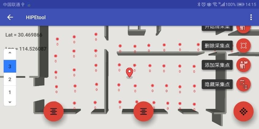
in previous subsection. An in-house application HIPE was developed for not only simultaneous indoor
positioning (see Figure 11 upper panel) but also for collecting Wi-Fi fingerprints along the reference
points in the offline phase (see Figure 11, the red dots on the bottom panel). Our indoor floor plan is
visualized by a commercial toolbox called Mapbox, which can be found at https://www.mapbox.com/.
In particular, we construct the indoor map in terms of the WGS-84 geodetic reference system [42]
to remain consistent with the outdoor map offered by Mapbox. In the positioning mode, our HIPE
application runs the Wi-Fi thread and PDR thread at the same time. The sampling rate of the IMU
sensor data is set to approximately 50 Hz (the “GAME” mode according to the Android API), and the
Wi-Fi scans continuously approximately every 2 s. In the radio map construction mode, the HIPE
application collects the Wi-Fi scan results at given reference points and simultaneously records the
corresponding coordinates through the Mapbox API, as shown in Figure 11. Additionally, we set
landmarks at each reference point, so that the ground truth positions of the user can be obtained
when the users record the timestamp and the number of landmarks they pass. In addition, a linear
interpolation of the landmarks’ positions is carried out to derive the pedestrian’s true position every
time when RSS updates.
Figure 11. Screenshots of HIPE application: the top panel denotes the online localization, and the
bottom panel denotes the construction of radio map.
We evaluate the HIPE application in a five-story office building, namely, Center of ShiLinTong,
which is owned by Wuhan University. The experiments were carried out in public areas on the third
floor with 75 m by 22 m in size, see Figure 12. The third floor is mainly composed of multiple meeting
rooms, teacher offices, student computer labs, lobbies and a long straight corridor (marked in white in
Figure 12). With this complex building structure, our experimental area includes most actual scenarios
in daily life, making it similar to the reality. In addition, as the building is in normal condition for
use, people are working routinely in their rooms and some occasionally walks around and passes by
our user when collecting fingerprint database in the offline phase. The situation in the online phase is
similar, so that the consistency of RSS measurements can be ensured. We note that the experiments (like
those in many previous literature) are carried out under some relatively ideal assumptions. For instance,
the surrounding people should be not too crowded, and the predefined paths for experiments are
selected to be as uniform as possible (see Figure 12). Otherwise, very crowded environments will
fail most of the state-to-art indoor positioning techniques including Wi-Fi fingerprinting, as far as
we know.Remote Sens. 2019, 11, 566 17 of 24
2001 2011
2010
2006 2007
2002 2003 2012 2013
2009
2004
2005
2008
Figure 12. Our Wi-Fi fingerprinting experimental testbed—all the training locations (reference points)
are marked as dark green points, and the office rooms are marked as the gray area. It is noted that the
areas in shadow are unavailable locations. The red curves denote the predefined paths (starting from
room 2005), which are designed along the reference points to ease the experiments.
We use two fingerprint-based localization approaches, the conventional RSS and the SSD
mentioned before, as benchmarks in our experiments. Based upon our experience, it is impractical to
dedicate vast amounts of computational and human resources to acquire data at each reference point to
construct the radio map for each approach. However, SSD and the proposed PSSD can be transformed
from an RSS-based radio map. In this context, we only need to collect data as required by the RSS
radio map in the offline training phase. Therefore, 219 reference points were established on a grid
map at intervals of approximately 2 m in public areas, such as the rooms and corridors, denoted as the
dark green dots in Figure 12. To establish a reliable conventional RSS fingerprint database, 30 sets of
sample data were first collected at each reference point by an Honor 8 smartphone, and subsequently,
the mean value of each AP RSSI at a given reference point constituted the RSS fingerprints. It should
be noted that the mean value was derived after removing the outliers with 3 − σ criteria. With the RSS
fingerprints, the SSD fingerprints can be easily established according to Equation (8).
As for the pairwise RSS fingerprint, we note that it is not directly derived from Equation (13),
because the pairwise fingerprint assumes the two points are connected (see Figure 8) while the walls
in our test environment divided the whole space into several separate subspaces such as the offices
and the corridor (see Figure 12). For example, a pairwise format between a point inside the office
and a point inside the corridor will lead to the cross-wall error. To this end, the pairwise RSS is first
constructed inside each subspace, which was numbered from 2001 to 2013 (see Figure 12), in addition
to the corridor. Subsequently, the pairwise RSS fingerprints built from each subspace were accumulated
as a whole, and this was the ultimate fingerprint database for later localization.
4.3. Overall Performance Evaluation
We first conducted experiments to verify our step count detection strategy, and during the
experiment, the pedestrian was asked to walk at a normal pace and fast pace. The analysis of the step
count error is shown in Table 1, and it should be noted that the true number of steps for each test
group was always 100. As can be seen from Table 2, the overall performance of our step count strategy
can ensure an accurate determination of the user’s walking speed (normal/fast) with the additional
timestamp information.Remote Sens. 2019, 11, 566 18 of 24
Table 2. Tests of step count detection.
Number of Tests Walk Speed Calculated Steps Steps Error Error Rate
1 Normal 98 2 2%
2 Normal 97 3 3%
3 Normal 97 3 3%
4 Fast 99 1 1%
5 Fast 100 0 0%
6 Fast 99 1 1%
Subsequently, another series of experiments were conducted to examine the robustness of PSSD
among heterogeneous smartphones as well as its possible superiority with respect to RSS/SSD
fingerprinting methods. Thus, the user was asked to hold the Samsung S8, Honor 8, and Huawei
P10 smartphones free from constraints on the walking speed. In addition, the user kept walking for
about ten minutes each time along the predefined paths that covered the test areas so that the ground
truth of pedestrians’ positions could be easily recorded. In addition, walking was repeated five times
at different times of the day to ensure that enough samples were collected to run the performance
evaluation. During the walk, all the Wi-Fi RSS scan results along with inertial sensor data were
recorded as inputs for the three algorithms. The cumulative distribution function (cdf) of localization
error is shown in Figure 13.
Figure 13a shows the test results of homogenous devices, where it can be found that the
RSS method achieves an average accuracy of 2.5 m (see Table 3) that might be not good enough.
We clarify that the causes of positioning errors may come from many sources, such as body blockage,
environmental change, device differences, and the other unknown factors. These error sources are
mostly varying and unpredictable, leading to a quasi-random error distribution without significant
patterns, in particular at a large building where no prior information of APs is known (this is our
case as well). In this sense, the positioning error (2.5 m) of RSS approach is reasonable, as it has no
particular treatment with any of the error sources. With one step further, the SSD has specifically
dealt with device difference problem, while the rest error sources remain. In contrast, rather than
dealing with each error source directly, the proposed PSSD approach bypasses them and imposes
the additional spatial constrain (user’s mobility as prior information) to the fingerprinting procedure,
so that the final positioning error can be reduced indirectly.
Unfortunately, the PSSD approach, which is developed from SSD, has completely inherited
the SSD’s ability to minimize device difference as well as SSD’s side effect on homogenous devices
discussed in previous subsection. Within expectation, a worse positioning performance of SSD and
PSSD than RSS approach in terms of homogenous devices can be found at Figure 13a and Table 2
(see the mean error). Figure 13a has shown that the RSS curve lies higher than the SSD curve at the
beginning, but eventually converges at the end, indicating that SSD performs slightly worse than
RSS and large errors still exist. In addition, the PSSD curve approximately overlaps the SSD curve,
but PSSD has slightly reduced the large errors regarding the SSD performance, as shown by the end
of their curves. The depicted results are also consistent with our previous inference that RSS should
perform best in terms of homogenous devices, but even in this case the PSSD has taken effect and
mitigated some large errors, as shown by the maximal error and 90 percentile error in Table 2.You can also read