An evaluation of the E3SMv1 Arctic ocean and sea-ice regionally refined model - GMD
←
→
Page content transcription
If your browser does not render page correctly, please read the page content below
Geosci. Model Dev., 15, 3133–3160, 2022
https://doi.org/10.5194/gmd-15-3133-2022
© Author(s) 2022. This work is distributed under
the Creative Commons Attribution 4.0 License.

An evaluation of the E3SMv1 Arctic ocean and sea-ice regionally
refined model
Milena Veneziani1 , Wieslaw Maslowski2 , Younjoo J. Lee2 , Gennaro D’Angelo1 , Robert Osinski3 , Mark R. Petersen1 ,
Wilbert Weijer1 , Anthony P. Craig4 , John D. Wolfe1 , Darin Comeau1 , and Adrian K. Turner1
1 Los  Alamos National Laboratory, Los Alamos, NM, USA
2 Naval  Postgraduate School, Monterey, CA, USA
3 Institute of Oceanology, Polish Academy of Sciences, Sopot, Poland
4 independent researcher

Correspondence: Milena Veneziani (milena@lanl.gov)

Received: 24 August 2021 – Discussion started: 8 October 2021
Revised: 24 February 2022 – Accepted: 15 March 2022 – Published: 12 April 2022

Abstract. The Energy Exascale Earth System Model                  the Arctic system relative to E3SM-LR-OSI, at a fraction
(E3SM) is a state-of-the-science Earth system model (ESM)         (15 %) of the computational cost of comparable global high-
with the ability to focus horizontal resolution of its multi-     resolution configurations, while permitting exchanges with
ple components in specific areas. Regionally refined global       the lower-latitude oceans that cannot be directly accounted
ESMs are motivated by the need to explicitly resolve, rather      for in Arctic regional models.
than parameterize, relevant physics within the regions of
refined resolution, while offering significant computational
cost savings relative to the respective cost of configurations
with high-resolution (HR) everywhere on the globe. In this        1   Introduction
paper, we document results from the first Arctic regionally
refined E3SM configuration for the ocean and sea-ice com-         The Arctic Ocean has been undergoing fundamental changes
ponents (E3SM-Arctic-OSI), while employing data-based at-         over the past several decades, which are best exemplified by
mosphere, land, and hydrology components. Our aim is an           a drastic year-round, and particularly summer, decline in sea-
improved representation of the Arctic coupled ocean and           ice coverage (Perovich et al., 2019). Given that sea-ice mod-
sea-ice state, its variability and trends, and the exchanges of   ulates the energy and property exchanges between the ocean
mass and property fluxes between the Arctic and the sub-          and atmosphere, the observed decline of sea-ice cover has
Arctic. We find that E3SM-Arctic-OSI increases the real-          impacted these interaction processes, their regional states,
ism of simulated Arctic ocean and sea-ice conditions com-         coupling, and associated variability. Some of the key impacts
pared to a similar low-resolution E3SM simulation without         of the sea-ice decline include an accumulation of heat ab-
the Arctic regional refinement in ocean and sea-ice compo-        sorbed in the upper Arctic Ocean (e.g., Timmermans et al.,
nents (E3SM-LR-OSI). In particular, exchanges through the         2018), due to reduced surface albedo and a related amplified
main Arctic gateways are greatly improved with respect to         warming of the lower atmosphere (e.g., Dai et al., 2019) rel-
E3SM-LR-OSI. Other aspects, such as the Arctic freshwater         ative to the globally averaged rate of warming in response
content variability and sea-ice trends, are also satisfactorily   to increasing CO2 . In addition, several studies have ascribed
simulated. Yet, other features, such as the upper-ocean strat-    the anomalous persistence of the anticyclonic Beaufort Gyre
ification and the sea-ice thickness distribution, need further    since 1997 until the present day – and the resulting contin-
improvements, involving either more advanced parameteri-          uous accumulation of freshwater within the Beaufort Gyre
zations, model tuning, or additional grid refinements. Over-      region – to the decline of sea ice (Proshutinsky et al., 2009;
all, E3SM-Arctic-OSI offers an improved representation of         Rabe et al., 2014; Haine et al., 2015; Proshutinsky et al.,
                                                                  2019). The freshwater accumulation in the Arctic Ocean and

Published by Copernicus Publications on behalf of the European Geosciences Union.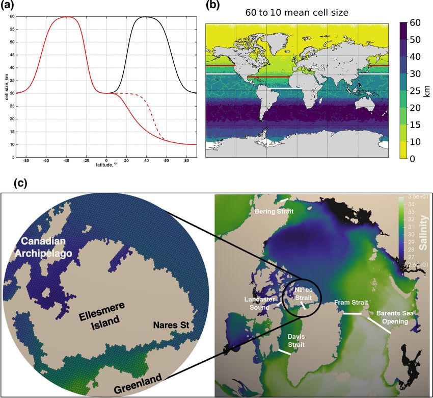
3134                                                M. Veneziani et al.: Evaluation of E3SM Arctic ocean and sea-ice model

its export through the Canadian Archipelago and Fram Strait        wards Arctic regional refinement in E3SM, which ultimately
is of relevance to the global ocean thermohaline circulation       will include comparable grid refinements in the atmosphere
because of its potential impact on convection and deep water       and land components of E3SM.
formation in the Greenland, Iceland, Irminger, and Labrador           The main objective of the paper is to investigate whether
seas (Häkkinen, 1993; Zhang et al., 2021).                         enhanced resolution in the Arctic and sub-Arctic translates
   Furthermore, the Arctic sea ice and climate are influenced      into an improved simulation of the sea-ice cover, the oceanic
by northward advection of warm water from the Pacific and          conditions, and the Arctic–sub-Arctic exchanges through the
Atlantic oceans. Polyakov et al. (2017) have recently intro-       main Arctic gateways. For the reasons mentioned previ-
duced the concept of “Atlantification” of the Arctic, recog-       ously in this section, we are interested not only in the pan-
nizing an increasing impact of incoming Atlantic waters en-        Arctic but also in the simulation of global and large-scale
tering the eastern basin through the Barents Sea Opening           metrics such as the Atlantic Meridional Overturning Circu-
(BSO) and Fram Strait on the sea-ice cover and the upper-          lation (AMOC). We achieve this main objective by com-
ocean stratification downstream, which acts to increase win-       paring E3SM-Arctic-OSI with a companion forced E3SM
ter ventilation in the ocean interior. Similarly, on the Pacific   ice–ocean simulation that uses a global low-resolution mesh
side, Woodgate and Peralta-Ferriz (2021) have reported an          (E3SM-LR-OSI). We also compare results with a high-
increasing inflow and warming of waters transported north-         resolution Regional Arctic System Model (RASM) simula-
ward across the Bering Strait during 1990–2019, which am-          tion when observations are scarce or unavailable. Due to the
plifies their impact on the ice regime downstream in the west-     higher number of constraints and its Arctic focus, we ex-
ern Arctic Ocean, where the ice has retreated furthest north       pect RASM to give a realistic representation of local pro-
in recent summers.                                                 cesses, while obviously not directly accounting for the Arc-
   The above examples and many other Arctic to midlatitude         tic to midlatitude exchange processes. This study is expected
exchange processes are inherently associated with feedbacks        to provide important insights to future model configurations
between various components of the Earth system, namely the         by the E3SM and by the broader Arctic modeling commu-
ocean, cryosphere, atmosphere, and land hydrology, and are         nity. A secondary objective of the present paper is to doc-
therefore better explored using a global, fully coupled Earth      ument Arctic-focused model evaluation metrics for E3SM.
system model (ESM). One such model is the recently devel-          This is accomplished through both common scripts for stan-
oped Energy Exascale Earth System Model (E3SM), spon-              dalone model-observation comparisons and by the addition
sored by the United States Department of Energy (Golaz             of Arctic metrics to the MPAS-Analysis package, which is a
et al., 2019). To our knowledge, there is only one other Arc-      Python-based analysis package developed at the Los Alamos
tic regionally refined ESM configuration to date, i.e., the Fi-    National Laboratory specifically for MPAS model compo-
nite Element Sea ice-Ocean Model (FESOM; Wekerle et al.,           nents1 .
2013, 2017a, b; Wang et al., 2018). The ocean and sea-ice             The paper is organized as follows: a description of the
model components of E3SM are based on the unstructured-            model configurations and simulations utilized throughout
grid Model for Prediction Across Scales (MPAS) frame-              the paper is included in Sect. 2. Results in terms of both
work; hence, they are particularly suited for focusing res-        global diagnostics and Arctic-focused metrics are presented
olution in specific regions toward explicitly resolving fine-      in Sects. 3–5. Finally, a discussion and conclusions are in-
scale physics, rather than parameterizing it, while retaining      cluded in Sect. 6.
the context of a global Earth System configuration (Ringler
et al., 2013; Petersen et al., 2019). In this study, we utilize
the E3SM-MPAS framework to evaluate the first regionally           2   Model configurations and simulations
refined E3SM Arctic ocean and sea-ice configuration with
                                                                   In this section, we provide some details of the following
a data-based atmosphere model component (E3SM-Arctic-
                                                                   three model configurations: E3SM-Arctic-OSI, E3SM-LR-
OSI), using 10 km horizontal resolution in the pan-Arctic re-
                                                                   OSI, and the RASM simulation.
gion and 10–60 km resolution elsewhere. A similar config-
                                                                      The ocean and sea-ice model components of E3SM are
uration to this, but with Arctic regional refinement of 6 km
                                                                   MPAS-Ocean and MPAS-Seaice (Petersen et al., 2019;
was also considered initially; that simulation, while being ap-
                                                                   Turner et al., 2021), respectively, and the two components
proximately 3 times more expensive than the one described
                                                                   share a common mesh that is typically made by hexagonal
in this paper, did not produce any significant improvements
                                                                   grid elements, although cells may have any number of sides.
in the Arctic and sub-Arctic ocean and sea-ice representation.
                                                                   The MPAS-Ocean vertical grid is structured and consists of
We concluded that a resolution of at least 3 km is necessary
                                                                   80 levels, with vertical resolution ranging between 2 m in the
to really resolve the local Rossby radius of deformation in
                                                                   upper 10 m of the water column and 200 m towards the ocean
most of the Arctic, and we plan to actively work on such
                                                                   bottom. The configurations presented here use z-star, where
very high-resolution E3SM-Arctic configurations in the near
future. While more specific studies using this model will fol-        1 https://mpas-dev.github.io/MPAS-Analysis/stable/ (last access:
low, we deem it important to document this first effort to-        5 April 2022)

Geosci. Model Dev., 15, 3133–3160, 2022                                             https://doi.org/10.5194/gmd-15-3133-2022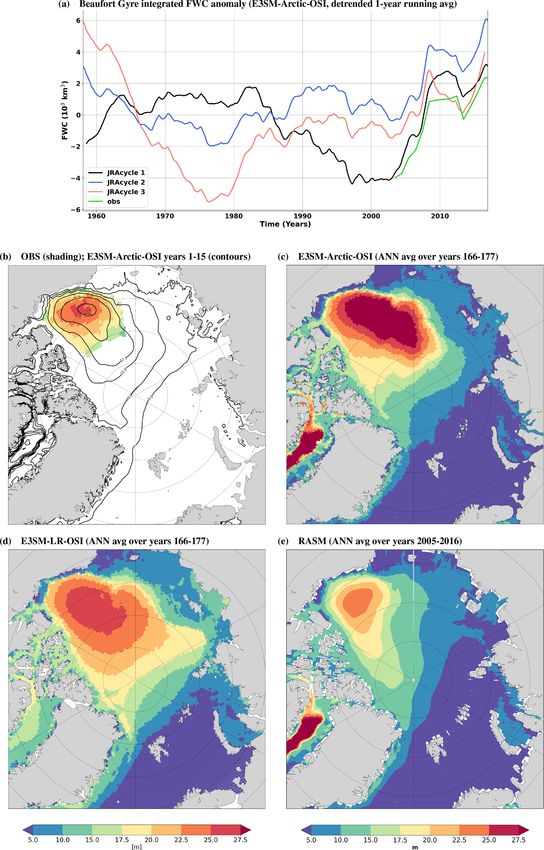
M. Veneziani et al.: Evaluation of E3SM Arctic ocean and sea-ice model                                                       3135

the layer thicknesses of the full column expand and contract       et al. (2019); we have not changed any default MPAS-Seaice
with the sea surface height (Adcroft and Campin, 2004; Pe-         parameter for the purposes of the present effort.
tersen et al., 2015). The ocean prognostic volume equation            The atmospheric data used to force the ocean and sea-ice
of state includes surface fluxes from the atmosphere and land      model components are the Japanese atmospheric reanalysis
via the coupler; thus, virtual salinity fluxes are not utilized.   product for driving ocean-sea-ice models (JRA55-do, ver-
   The E3SM-Arctic-OSI configuration has a horizontal res-         sion v1.3; Tsujino et al., 2018). At the time of our simula-
olution of 10 km in the Arctic Ocean, whereas, in the South-       tions, the JRA55-do atmosphere fluxes and river runoff data
ern Hemisphere, it has the nominal horizontal resolution           set was available for the period 1958–2016. The JRA55 prod-
of 1◦ that is the E3SM standard low resolution used in             uct has a temporal resolution of 3 h and a horizontal reso-
E3SM-LR-OSI and in the model study of Golaz et al. (2019)          lution of 0.5625◦ , which is more than 3 times higher than
(Fig. 1b). As seen in Fig. 1a (red curves), the mesh resolution    the resolution of the Coordinated Ocean-ice Reference Ex-
transitions from 60 km in the Southern Hemisphere to 30 km         periment (CORE; Griffies et al., 2009) data used in forced
in the tropics to 10 km north of 60◦ N (for this reason, the       ice–ocean ESM simulations until recently. Following Griffies
E3SM-Arctic-OSI mesh is also referred to as 60to10). The           et al. (2009), sea surface salinity (SSS) is restored to monthly
horizontal resolution transitions to smaller grid cells more       climatological values obtained from the Polar science cen-
quickly in the Atlantic than in the Pacific Ocean (compare         ter Hydrographic Climatology (PHC3.0; updated from Steele
solid versus dashed lines in Fig. 1a), ensuring that (i) the       et al., 2001), with an equivalent restoring timescale of 1 year.
Gulf Stream extension region (around 40◦ N) is character-             The E3SM-LR-OSI configuration is similar to E3SM-
ized by a resolution of at least 15 km, and (ii) that the subpo-   Arctic-OSI in terms of atmospheric forcing, but it uses the
lar North Atlantic (north of 50◦ N) has a resolution similar to    standard global low-resolution mesh (black curve in Fig. 1a)
the one in the Arctic (around 10–12 km). Figure 1c shows a         and 60 vertical levels, with vertical resolution ranging be-
zoom-in of the E3SM-Arctic-OSI mesh over the Arctic and            tween 10 m in the upper 200 m of the water column and
subpolar North Atlantic region, with a further enlargement         250 m below 3000 m depth. In this case, the GM parameter-
inset displaying the hexagonal cells in more detail. The to-       ization is on at all latitudes. The ocean baroclinic time step
tal number of cells is 0.62 million and the computational          is equal to 30 min. Key features of the E3SM configurations
cost is 1.65 million CPU hours per simulated century. In           described above (and of the RASM simulation) have been
comparison, the global high-resolution E3SM configuration          summarized and compared against those described in three
(E3SM-HR; Caldwell et al., 2019) has a computational cost          previous E3SM publications in Table 1.
of 11.17 million CPU hours per simulated century (Petersen            We have performed two simulations consisting of three
et al., 2019); therefore, the E3SM-Arctic-OSI computational        consecutive JRA cycles: one using E3SM-Arctic-OSI and
cost is about 15 % of the computational cost of E3SM-HR.           one using E3SM-LR-OSI. The choice of three cycles was
   The ocean baroclinic time step is equal to 10 min. Ocean        mostly constrained by the availability of computational re-
vertical mixing is parameterized through the K-profile pa-         sources when these simulations were performed. We also
rameterization method (KPP; Large et al., 1994), and no            compared trends of fields of interest during the second and
background vertical diffusivity is utilized. Mesoscale eddy        third cycles, and, as the results shown later in the paper will
effects are represented using the Gent–McWilliams (GM)             elucidate, we were sufficiently satisfied that such trends re-
eddy transport parameterization of Gent and McWilliams             mained mostly stable between the second and third cycle.
(1990) in regions outside of the Arctic and pan-Arctic. To         In both simulations, the ocean is initialized from a 1-month
achieve this regionally varying application of GM, a simple        spin up from rest, to allow for initial gravity waves adjust-
algorithm has been implemented in MPAS-Ocean for which             ment, and from a temperature and salinity initial condition
the GM parameter is a ramp-like function of grid cell size.        obtained from the PHC January climatology. Sea ice is ini-
In particular for the E3SM-Arctic-OSI configuration consid-        tialized with a 1 m thick disk of sea ice extending to 60◦ N
ered here, the GM kappa parameter varies linearly between          and S.
zero for cell sizes below 20 km and a maximum value of                RASM is a fully coupled, limited-area ESM, which has
600 m2 s−1 for cell sizes above 30 km. This means that we          been used for dynamic downscaling of global atmospheric
effectively transition from GM-on to GM-off in the North           reanalyses as well as ESM projections (Maslowski et al.,
Atlantic within ≈ 10–28◦ N and approximately within 25–            2012; Roberts et al., 2015; Hamman et al., 2016; Cassano
50◦ N elsewhere (see areas between the white and red lines         et al., 2017; Brunke et al., 2018). It includes the Weather Re-
in Fig. 1b). In other words, the GM kappa is 0 for latitudes       search and Forecasting (WRF) atmosphere model, the Par-
above the red line and is equal to its maximum 600 m2 s−1 for      allel Ocean Program (POP) ocean component, the Commu-
latitudes below the white line. Other parameterizations used       nity Ice Model (CICE) sea-ice component, and the Variable
in MPAS-Ocean are invariable with horizontal resolution.           Infiltration Capacity (VIC) land hydrology model. A source-
   The version of MPAS-Seaice used in this paper and the           to-sink river-routing model (RVIC) allows coupling of the
way that the sea-ice and ocean components are coupled to-          land hydrology and ocean components. All these compo-
gether are fully described in Turner et al. (2021) and Petersen    nent models are coupled every 20 min using a version of

https://doi.org/10.5194/gmd-15-3133-2022                                             Geosci. Model Dev., 15, 3133–3160, 2022
3136                                                  M. Veneziani et al.: Evaluation of E3SM Arctic ocean and sea-ice model

Figure 1. (a) Distribution function used to define cell size as a function of latitude and create the meshes: red curves indicate the E3SM-
Arctic mesh, whereas the black curve indicates the E3SM-LR mesh. The solid red line marks resolution changes in the Atlantic Ocean and
the dashed red line marks changes in the Pacific Ocean. Note that all lines converge (same behavior everywhere for both E3SM-Arctic and
E3SM-LR) in the Southern Hemisphere. (b) Geographical distribution of grid cell size for the E3SM-Arctic-OSI configuration. The area
between the white and red lines denotes the region where the transition between GM-on and GM-off occurs (no GM eddy parameterization
is used north of the red lines). (c) Zoom-in around the Arctic of a salinity field simulated in E3SM-Arctic-OSI, with a further enlargement
around Ellesmere Island to show the hexagonal mesh in more detail. Also shown are the locations of the five Arctic gateways and Davis
Strait, through which fluxes in and out of the Arctic are later calculated.

Table 1. Main configuration differences between the model experiments described in this paper and those described in key E3SMv1 (ver-
sion 1) publications. Numbers used in the “horizontal mesh” column refer to the minimum and maximum resolutions in kilometers for E3SM
cases, while we have indicated that a regular 9 km resolution mesh is used for the RASM case.

       Study                    Model                Atmospheric forcing     Horizontal mesh     Vertical levels   GM
                                E3SM-Arctic-OSI      JRA55-do                Arctic 60to10             80          On outside Arctic
       This paper               E3SM-LR-OSI          JRA55-do                60to30                    60          Fully on
                                RASM                 JRA55-do                Regular 9 km              45          Fully off
                                E3SMv1-HR-OSI        CORE-II                 18to6                     80          Fully off
       Petersen et al. (2019)
                                E3SMv1-LR-OSI        CORE-II                 60to30                    60          Fully on
       Golaz et al. (2019)      E3SMv1-LR            Coupled                 60to30                    60          Fully on
       Caldwell et al. (2019)   E3SMv1-HR            Coupled                 18to6                     80          Fully off

Geosci. Model Dev., 15, 3133–3160, 2022                                                  https://doi.org/10.5194/gmd-15-3133-2022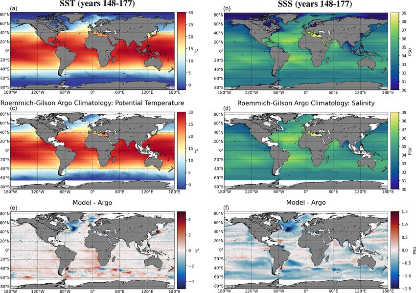
M. Veneziani et al.: Evaluation of E3SM Arctic ocean and sea-ice model 3137
the CESM coupler, CPL7, modified for a regional applica-
tion. The model domain covers the entire pan-Arctic region
(extending down to ≈ 45◦ N in the North Atlantic and to
≈ 30◦ N in the North Pacific), including the entire marine
cryosphere of the Northern Hemisphere as well as terrestrial
drainage to the Arctic Ocean and its margins. The RASM
configuration used for the model intercomparison in Sects. 4
and 5 has a horizontal resolution of 9 km (i.e., 1/12◦ in a
rotated spherical coordinate system) throughout the domain
with 45 vertical levels. The sea-ice component shares the
same horizontal resolution as the ocean and it is configured
with five ice thickness categories. The RASM ocean temper-
ature and salinity along the closed lateral boundaries are re-
stored to the monthly PHC3.0 climatology. No lateral bound-
ary conditions for sea ice are required given the extent of
the pan-Arctic domain. The RASM results used in this paper
are from an ocean–sea-ice simulation forced with JRA55-
do, which in turn was initialized from a 75-year long spinup
forced with the Coordinated Ocean-ice Reference Experi-
ments Corrected Inter-Annual Forcing version 2.0 (CORE2-
CIAF); here, we focus on the last 40 years (1979–2018) of
this run.
3 Global ocean
The purpose of this section is to describe how the E3SM-
Arctic-OSI simulation represents climatologies and trends of
key global ocean fields. The global trend of OHC anomaly
for three depth ranges, and of T and S as a function of depth,
are presented in Fig. 2. Anomalies are computed relative to
the first-year annual means and are 1-year running-averaged
to filter out the seasonal cycle. At the end of the third JRA
cycle, the T and S distribution is only slightly trending in the Figure 2. Global trends for the E3SM-Arctic-OSI simulation of
500–1000 m depth range. Alternating bands of warming and (a) ocean heat content (OHC) anomalies integrated over the full
cooling are found in the upper 2000 m of the global water depth column (thick solid line) and over the following depth ranges:
column (Fig. 2b), although the OHC for the 0–700 m depth 0–700 m (thin solid line), 700–2000 m (dashed line), and 2000 m–
range indicates a net warming for the upper ocean (Fig. 2a). bottom (plus line); (b) temperature and (c) salinity anomalies as a
On the other hand, the bottom waters deeper than 4000 m ex- function of depth. Anomalies are computed with respect to the first-
year annual mean and are 1-year running averages.
hibit a cooling persistent anomaly of up to 0.5 ◦ C. Salinity
experiences a more regular change with depth, with a fresh-
ening of up to 0.2 psu in the upper 800 m and a salinification
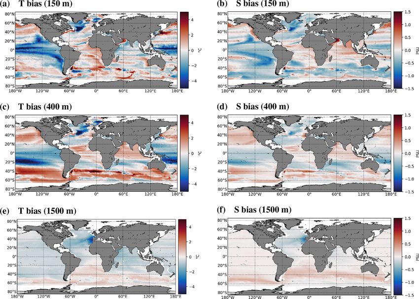
of up to 0.1 psu in the deeper ocean (Fig. 2c). Overall, the drastic reduction of the biases in the upper 1000 m ocean
top-to-bottom trends are all reduced during the third cycle, stratification, mainly in the Southern Ocean and Labrador
whereas the upper-ocean warming and freshening are both Sea (not shown, unpublished results). T and S biases are
still present towards the end of the simulation. much reduced below 1000 m (Fig. 4e and f).
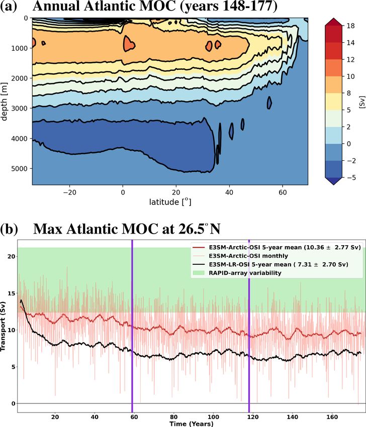
When comparing the model global T and S with obser- Another important indication of the state of a global ESM
vations (from the Roemmich–Gilson Argo data; Roemmich is the AMOC. To that effect, the E3SM-Arctic-OSI overturn-
and Gilson, 2009) at different depths (surface, 150, 400, and ing streamfunction plot as a function of latitude as well as
1500 m) in Figs. 3–4, we mostly note the generally fresh bias the time series of maximum AMOC at 26.5◦ N for both the
in the upper 150 m, especially evident south of 40◦ S and in E3SM-Arctic-OSI and E3SM-LR-OSI are shown in Fig. 5.
the North Atlantic at the surface, but also in the tropical Pa- Observational variability from the Rapid Climate Change-
cific at 150 m. This behavior is consistent with biases docu- Meridional Overturning Circulation and Heat-flux Array
mented in Golaz et al. (2019). Recent improvements in the (RAPID-MOCHA) data set (Cunningham et al., 2007; Mc-
MPAS-Ocean eddy parameterization scheme have led to a Carthy et al., 2020) is shaded in green for reference. While
https://doi.org/10.5194/gmd-15-3133-2022 Geosci. Model Dev., 15, 3133–3160, 2022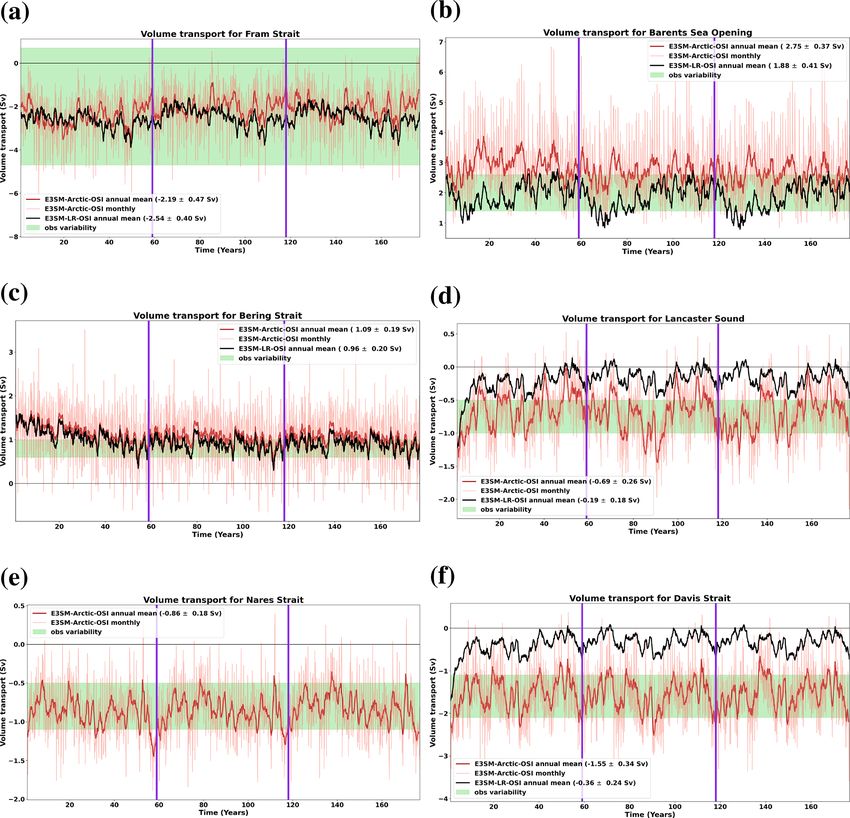
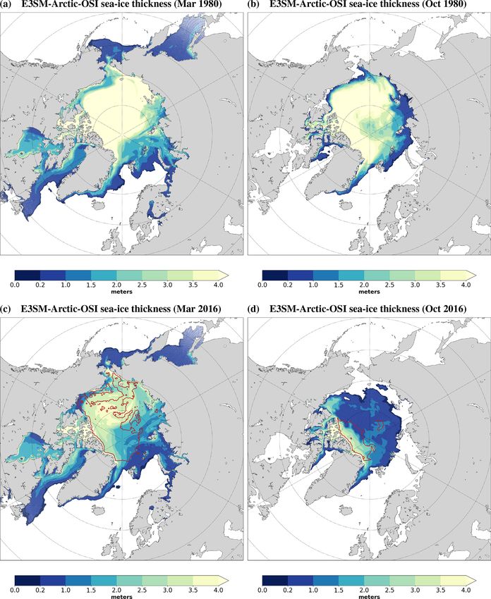
3138                                                M. Veneziani et al.: Evaluation of E3SM Arctic ocean and sea-ice model

Figure 3. SST (a, c, e) and SSS (b, d, f) from the E3SM-Arctic-OSI simulation (a, b) and the Roemmich–Gilson Argo climatological data
set (c, d). The corresponding model minus observation bias is shown in panels (e) and (f). Model climatologies are computed over years
148–177 (last 30 years of the third JRA cycle).

we have a reasonable (albeit on the strong side) Antarctic           sented in Fig. 6, which shows a meridional vertical section
Bottom Water cell of 2–4 Sv (e.g., Orsi et al., 2002), the up-       of zonally averaged salinity in the Atlantic Ocean (north of
per cell of the AMOC at 26.5◦ N is weaker than observa-              Fram Strait the average is computed over the whole Arc-
tions by ≈ 6 Sv in E3SM-Arctic-OSI and is reduced by an              tic) with overlapped contours of sigma2 (potential density
additional 3 Sv in E3SM-LR-OSI (the average value from               with respect to 2000 m). The fields are interannual averages
RAPID over the period 2004–2017 is 16.8 ± 4.4 Sv; Mc-                computed over years 148–177. Two main features emerge
Carthy et al., 2020). A weak AMOC in other low-resolution            from Fig. 6: (i) a less fresh North Atlantic north of 65◦ N
E3SM simulations has been reported previously (Golaz et al.,         (Nordic Seas) in E3SM-Arctic-OSI compared to E3SM-LR-
2019; Weijer et al., 2020). Although a thorough investiga-           OSI, also associated with a deeper reaching convection in
tion of its causes is beyond the purposes of this paper, we          the same area (see missing or greatly reduced slumping of
hypothesize that improved SSS and ocean stratification in            sigma2 isopycnals between 65 and 75◦ N in the E3SM-LR
the subpolar North Atlantic and in the Southern Ocean has            third panel); (ii) a steeper Southern Ocean stratification in
an important impact on E3SM deep high-latitude convection            E3SM-Arctic-OSI, which causes Circumpolar Deep Water
and on its AMOC. SSS biases calculated similarly to Fig. 3           associated with sigma2 of 36.8–37 kg m−3 to remain well be-
but for the E3SM-LR-OSI (not shown) are more than 1 psu              low the surface in E3SM-LR-OSI. Both of these features are
fresher than those for E3SM-Arctic-OSI in the Nordic Seas            consistent with the presence of a stronger AMOC in E3SM-
region, and that is associated with higher mixed layer depth         Arctic compared to E3SM-LR and, partially, with the results
biases (not shown) with respect to an Argo floats’ derived           of Bryan et al. (2014).
observational product. Such differences in stratification be-           While we acknowledge the global biases discussed in this
tween E3SM-Arctic-OSI and E3SM-LR-OSI are clearly pre-               section, we also note that they fall within the published inter-

Geosci. Model Dev., 15, 3133–3160, 2022                                               https://doi.org/10.5194/gmd-15-3133-2022
M. Veneziani et al.: Evaluation of E3SM Arctic ocean and sea-ice model                                                                       3139

Figure 4. Model minus observation bias for (a, c, e) temperature and (b, d, f) salinity at depths of (a, b) 150 m, (c, d) 400 m, and (e, f) 1500 m.
Biases are computed similarly to the lower panels of Fig. 3 and for model climatologies over years 148–177.

model spread of results from forced climate models (Dan-                    Archipelago (and eventually the Davis Strait), and through
abasoglu et al., 2014; Tsujino et al., 2020). Furthermore,                  the Fram Strait. Observational values of the volume trans-
as we discuss in the next sections, the E3SM-Arctic-OSI                     port (and heat and freshwater transport, when available)
simulation of the Arctic is satisfactory, and improvements                  through these gateways vary according to the time period
in MPAS-Ocean and MPAS-Seaice introduced in E3SMv2                          over which the observations were actually taken. Typically
are expected to yield further improvements in future E3SM-                  cited numbers for the volume transport include a net inflow of
Arctic simulations of global and high-latitude climate.                     2±0.6 Sv through the BSO (based on measurements between
                                                                            1997 and 2007, from Skagseth et al., 2008, and Smedsrud
                                                                            et al., 2013); a net inflow through Bering Strait of 0.8±0.2 Sv
4   Arctic gateways                                                         (1990–2007, from Woodgate and Aagaard, 2005); a net out-
                                                                            flow through the Fram Strait of 2 ± 2.7 Sv (1997–2007, from
Given the importance of the Arctic–sub-Arctic ocean ex-
                                                                            Schauer et al., 2008); and a net outflow through the Davis
changes to regional and global climate change, we exam-
                                                                            Strait of 1.6 ± 0.5 Sv (2004–2010, from Curry et al., 2014).
ine the multi-year mean simulated ocean fluxes across the
                                                                            Observations are also available in key channels of the Cana-
five main gateways that connect the Arctic Ocean with
                                                                            dian Archipelago, such as Lancaster Sound and Nares Strait
the subpolar North Atlantic and North Pacific Oceans (see
                                                                            (Fig. 1c), but they are over shorter time records (see captions
Beszczynska-Möller et al., 2011, for an overview). Warm
                                                                            of subsequent figures and Table 2 for references to specific
and salty water of Atlantic origin enters the Arctic through
                                                                            studies).
the BSO and Fram Strait, while warm and freshwater of Pa-
                                                                               In the remainder of this section, we focus on how the
cific origin flows into the Arctic through the Bering Strait.
                                                                            model reproduces exchanges of volume, heat, and liquid
The outflow of water from the Arctic takes place through
                                                                            freshwater through the above-mentioned Arctic gateways.
the Nares Strait and Northwest Passages in the Canadian

https://doi.org/10.5194/gmd-15-3133-2022                                                        Geosci. Model Dev., 15, 3133–3160, 2022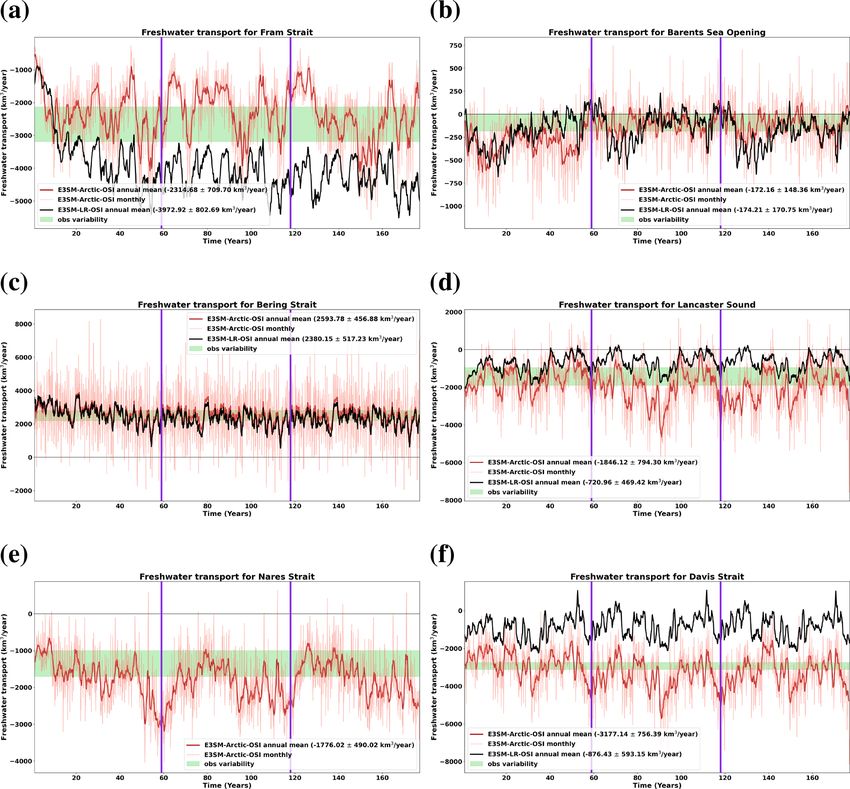
3140                                                    M. Veneziani et al.: Evaluation of E3SM Arctic ocean and sea-ice model

                                                                        able); for the freshwater transport, 34.8 psu is used as the
                                                                        reference salinity, since that is the common reference used
                                                                        in Arctic observational studies. The sign convention for this
                                                                        transport is such that positive values imply net fluxes into the
                                                                        Arctic Ocean, and negative values imply net fluxes out of the
                                                                        Arctic.
                                                                           The Fram Strait and BSO are two important gateways both
                                                                        in terms of heat and freshwater transport into and out of the
                                                                        Arctic: the E3SM-Arctic-OSI simulation reproduces well the
                                                                        mean volume, heat, and freshwater transport through these
                                                                        gateways compared to observations (red lines in Figs. 7a and
                                                                        b, 8a and b, 9a and b, and mean values in first two rows
                                                                        of Table 2). While the net volume transport through these
                                                                        two gateways is not characterized by an appreciable trend
                                                                        over each JRA cycle, the net heat transport through both
                                                                        the Fram Strait and the BSO exhibits an upward trend over
                                                                        the last ≈ 40 years of each cycle (Fig. 8a and b), and the
                                                                        net freshwater transport through the BSO exhibits a down-
                                                                        ward trend over the same time period (Fig. 9b; note that
                                                                        less negative freshwater flux effectively means that the Arc-
                                                                        tic is losing less freshwater with respect to 34.8 psu through
                                                                        the BSO). These results are in agreement with observa-
                                                                        tional studies such as Skagseth et al. (2008), Schauer et al.
                                                                        (2008), and Polyakov et al. (2017), promoting the idea of
Figure 5. (a) Annual MOC streamfunction computed over the At-           “Atlantification” of the Arctic, with warmer and saltier At-
lantic Ocean and over years 148–177 of the E3SM-Arctic-OSI sim-         lantic Water flowing into the Arctic in recent decades. The
ulation (black contours are every 2 Sv); (b) time series of the 5-      simulated net freshwater transport through the Fram Strait
year running average maximum Atlantic MOC detected at 26.5◦ N           is more variable and follows quite closely the observational
(latitude of the RAPID-MOCHA observational array) from E3SM-            record of the Norwegian Polar Institute (de Steur et al., 2009;
Arctic-OSI (dark red line) and E3SM-LR-OSI (black line). The
                                                                        de Steur, 2018, see also graph at http://www.mosj.no/en/
light red line shows E3SM-Arctic-OSI monthly values. The num-
bers shown in the insets are the mean and standard deviations of
                                                                        climate/ocean/freshwater-flux-fram-strait.html, last access:
the annual model values, computed over the full time series. The        7 April 2022). Net volume fluxes through the Fram Strait
RAPID array typical variability (16.8 ± 4.4 Sv) is shaded in green.     and the BSO are also well reproduced in E3SM-LR-OSI,
Finally, the purple vertical lines show the transition across JRA cy-   but net heat transport is ∼ 4 times weaker through the Fram
cles.                                                                   Strait and 38 % weaker through the BSO than E3SM-Arctic-
                                                                        OSI. The Fram Strait is also characterized by an almost
                                                                        twice as intense net freshwater export with respect to the
Full time series of the net fluxes are presented in Figs. 7–9,          E3SM-Arctic-OSI results (and observations; see black lines
and mean values are summarized in Table 2. They are com-                in Fig. 9a and Table 2).
pared with available observations and with the multi-model                 The Lancaster Sound and Nares Strait (Fig. 1c) are the
studies of Ilicak et al. (2016) and Wang et al. (2016a). It             only connections from the Arctic to Baffin Bay through the
should be noted that integrated long-term observational vol-            Canadian Archipelago, since both the Cardigan Strait and
ume flux estimates yield an imbalance of 0.8 Sv (per Table 2),          Hell Gate, two small Northwestern Passages to the north of
while the respective model integrated volume estimates are              Lancaster Sound, are closed in our E3SM-Arctic-OSI con-
by definition close to zero (< 0.1 Sv), which complicates               figuration. On average, the net volume transport through
comparison of fluxes at individual gates. In addition, a full           these two gateways compares very well with available ob-
volume, heat, and freshwater budget of the Arctic is beyond             servations, and their sum defines the mean volume transport
the scope of this paper. Finally, we acknowledge that esti-             through the Davis Strait (Fig. 7d–f). While net heat trans-
mates of heat and freshwater fluxes across an individual sec-           port through the Lancaster Sound and Nares Strait is very
tion are sensitive to the respective reference values used for          small compared to the other gateways, heat flux through the
temperature and salinity, but we argue that their accumulated           Davis Strait is almost 1 order of magnitude higher (≈ 10 TW
quantities for a closed volume are justified. For the heat trans-       on average), suggesting that there is a substantial heat loss
port calculations, either the freezing point or 0 ◦ C is used as        to the atmosphere in Baffin Bay. The Canadian Archipelago
the reference temperature, depending on the reference used              gateways are most important for the transport of freshwa-
by the corresponding observational estimate (where avail-               ter out of the Arctic (Fig. 9d and e). Similarly to the Fram

Geosci. Model Dev., 15, 3133–3160, 2022                                                 https://doi.org/10.5194/gmd-15-3133-2022
M. Veneziani et al.: Evaluation of E3SM Arctic ocean and sea-ice model                                                                 3141

Figure 6. Meridional vertical section of zonally averaged salinity field, where the zonal average is computed over the Atlantic sector of the
global ocean and over the whole Arctic Ocean north of approximately the latitude of Fram Strait, from (a) E3SM-Arctic-OSI and (b) E3SM-
LR-OSI. Contour lines follow the sigma2 field (potential density with respect to 2000 m). All fields are climatologies over years 148–177.

Strait, the freshwater transport through the Lancaster Sound             E3SM-LR-OSI of potential temperature, salinity, and normal
and Nares Strait exhibits substantial interannual and decadal            velocity for the Fram Strait, BSO, Davis Strait, and Bering
variability, something that is not fully captured by observa-            Strait, respectively (Table 2 also includes the averaged val-
tions, likely due to the limited coverage of these records (the          ues of incoming and outgoing transport for all fluxes). The
observational range is based on the 1998–2001 record in Lan-             model climatologies are computed over the last 12 years of
caster Sound from Prinsenberg and Hamilton, 2005 and on                  the third JRA cycle. A comparison with climatologies com-
the 2003–2009 record in the Nares Strait from Münchow,                   puted on an analogous period of the first cycle (not shown)
2016). Because of the low horizontal resolution and the fact             indicates that, while some T and S changes are apparent be-
that the Nares Strait is closed in E3SM-LR-OSI, net volume               low the Atlantic Water layer in Fram Strait and the BSO, and
transport through the Lancaster Sound is not significantly               in the West Greenland Current in the Davis Strait, the over-
different from 0, and all net fluxes through the Davis Strait            all structure of the gateways stratification is quite consistent
are much reduced (by up to 3 times) in E3SM-LR-OSI com-                  between the first and third JRA cycles, and consequently the
pared with E3SM-Arctic-OSI results and observations. Note                velocity structures are also very comparable.
from Table 2 that this reduction of outward volume trans-                   The Fram Strait results in terms of the cross section of
port through the Davis Strait in E3SM-LR-OSI with respect                temperature and normal velocity (Fig. 10a and e) are com-
to E3SM-Arctic-OSI is partly compensated by an increase in               pared with the 2002–2008 observational climatologies in
transport through the Fram Strait but also by a decrease in              Beszczynska-Möller et al. (2012, their Fig. 2), whereas the
transport into the Arctic through the BSO and Bering Strait.             salinity cross section (Fig. 10c) can be compared with 1997
   The two simulations interestingly reproduce the net fluxes            observations in Rudels (2012, his Fig. 20). They show a
through the Bering Strait similarly (panel c in Figs. 7–9),              good representation of the currents and exchanges through
with volume and freshwater transport well represented com-               the strait. In particular, the West Spitsbergen Current carry-
pared with observations, and net heat transport on the lower             ing warm and salty modified Atlantic Water into the Arctic
end of observational estimates as also found in other ESM                west of the Svalbard Islands, besides being weaker in its core
studies (Ilicak et al., 2016). Furthermore, we note a down-              and warmer by ≈ 1 ◦ C in the western side of the section com-
ward trend in the net freshwater flux over the last 20 years of          pared with observations, exhibits a good vertical structure as
each JRA cycle (corresponding to the period ∼ 2006–2016;                 well as reasonable temperature and salinity ranges. The same
Fig. 9c), which is opposite to the observed upward trend re-             is true for the East Greenland Current carrying cold and fresh
ported in Woodgate (2018).                                               polar waters out of the Arctic along the Greenland shelf. Note
   While the net transport through the Arctic gateways pro-              that the West Spitsbergen Current carries slightly less water
vides useful diagnostics, it is equally important for a model            into the Arctic than what the East Greenland Current carries
to reproduce inflows and outflows, since those are associated            out of the Arctic, but the former is responsible for a net input
with different water masses and their impacts downstream                 of heat and the latter is responsible for a net loss of freshwa-
are commonly independent from each other. Figures 10–                    ter for the Arctic Ocean (see Table 2).
13 show vertical sections from both E3SM-Arctic-OSI and

https://doi.org/10.5194/gmd-15-3133-2022                                                     Geosci. Model Dev., 15, 3133–3160, 2022
3142                                                  M. Veneziani et al.: Evaluation of E3SM Arctic ocean and sea-ice model

Figure 7. Time series of the 1-year running average net volume transport for the five Arctic gateways (Fram Strait, BSO, Bering Strait,
Lancaster Sound, and Nares Strait) and Davis Strait, from E3SM-Arctic-OSI (dark red lines) and E3SM-LR-OSI (black lines). The light red
lines show E3SM-Arctic-OSI monthly values; the corresponding E3SM-LR-OSI monthly values are not shown for clarity. The vertical purple
lines mark the transition between JRA cycles. The numbers shown in the insets are the mean and standard deviations of the annual model
values, computed over the full time series. Transect location is displayed in Fig. 1c. Observational values are −2 ± 2.7 Sv for Fram Strait
(Schauer et al., 2008), 2 ± 0.6 Sv for the BSO (Skagseth et al., 2008; Smedsrud et al., 2013), 0.8 ± 0.2 Sv for the Bering Strait (Woodgate
and Aagaard, 2005), −0.75 ± 0.25 Sv for the Lancaster Sound (Prinsenberg and Hamilton, 2005), between −0.5 and −1.1 Sv for the Nares
Strait (Münchow, 2016), and −1.6 ± 0.5 Sv for the Davis Strait (Curry et al., 2014).

   The Fram Strait stratification and cross-section velocity in         the Arctic. These temperature and salinity profiles in E3SM-
E3SM-LR-OSI look very different: the upper 500 m of the                 LR-OSI may also explain the excessive net freshwater flux
water column is much more stratified than E3SM-Arctic-                  and reduced net heat flux through the Fram Strait discussed
OSI, exhibiting a very fresh and cold lens in the top 100 m             above.
that may be associated with an excessive sea-ice export out of

Geosci. Model Dev., 15, 3133–3160, 2022                                                  https://doi.org/10.5194/gmd-15-3133-2022
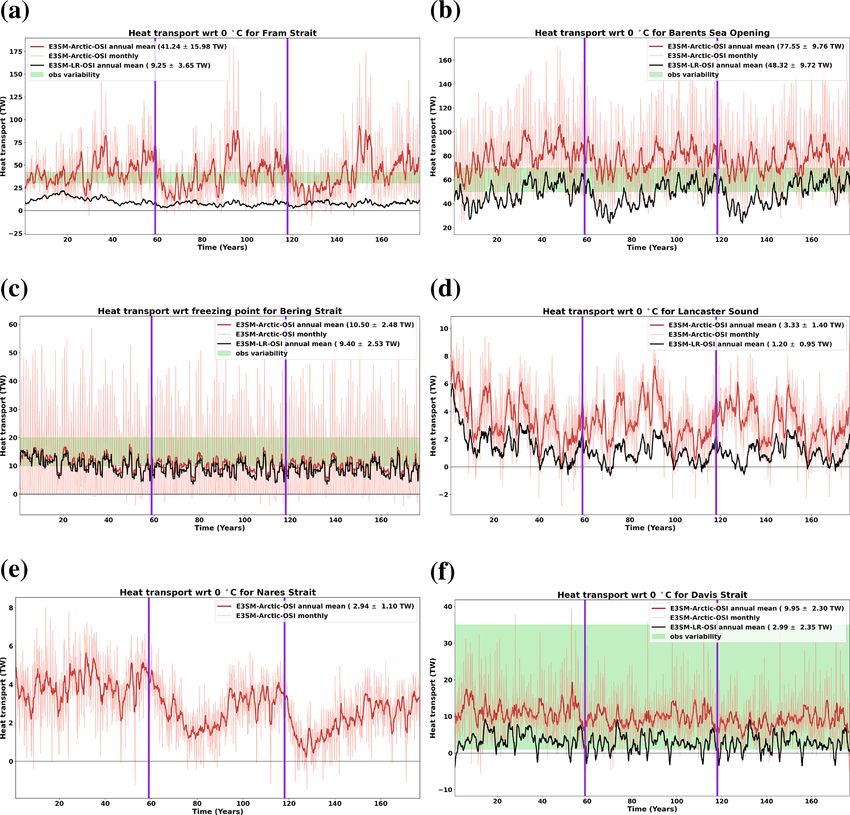
M. Veneziani et al.: Evaluation of E3SM Arctic ocean and sea-ice model                                                                      3143

Figure 8. Similar to Fig. 7 but for net heat transport, which is computed with respect to the 0 ◦ C reference temperature in panels (a), (b), (d)–
(f), and with respect to the freezing point in panel (c). Observational ranges, where available, are shaded in green; their values are 36 ± 6 TW
for the Fram Strait (Schauer and Beszczynska-Möller, 2009), between 50 and 70 TW for the BSO (Smedsrud et al., 2010), between 10 and
20 TW for the Bering Strait (Woodgate et al., 2010, these authors use the freezing point as reference temperature, as done for the model
estimates), and 18 ± 17 TW for the Davis Strait (Cuny et al., 2005).

   Since the bulk of the water flowing across the BSO                      the Arctic through the BSO is slightly fresher and colder, but
has salinities greater than the reference salinity of 34.8 psu             the slope and interior currents are well simulated in terms
(Fig. 11d), this represents freshwater export from the Arctic              of both horizontal and vertical structure (Fig. 11a, c, e). The
(see negative values for both net and incoming freshwater for              corresponding results for E3SM-LR-OSI (Fig. 11b, d, f) are
the BSO in Table 2). Compared with observations (Fig. 3 in                 also acceptable, although they exhibit a weaker Norwegian
Skagseth et al., 2008, which in truth only represents condi-               Atlantic Current than in E3SM-Arctic-OSI and observations.
tions for August 1998, while the model results are interan-                   The Davis Strait temperature and salinity cross sections
nual climatologies), the model Atlantic Water flowing into                 are also well simulated in E3SM-Arctic-OSI (the results,

https://doi.org/10.5194/gmd-15-3133-2022                                                        Geosci. Model Dev., 15, 3133–3160, 2022
3144                                                   M. Veneziani et al.: Evaluation of E3SM Arctic ocean and sea-ice model

Figure 9. Similar to Fig. 7 but for net freshwater transport, where freshwater is computed with respect to the reference salinity of 34.8 psu.
Observational values are −2660 ± 528 km3 yr−1 for the Fram Strait and −90 ± 94 km3 yr−1 for the BSO (see Serreze et al., 2006, for
both estimates), 2500 ± 300 km3 yr−1 for the Bering Strait (Woodgate and Aagaard, 2005), between −1900 and −950 km3 yr−1 for the
Lancaster Sound (Prinsenberg and Hamilton, 2005), between −1700 and −1000 km3 yr−1 for the Nares Strait (Münchow, 2016), and
−2930 ± 190 km3 yr−1 for the Davis Strait (Curry et al., 2014).

seen in Fig. 12a and c, are compared with Tang et al., 2004,             5    Arctic Ocean and sea-ice conditions
their Fig. 4), whereas a strong stratification caused by a low-
salinity upper 150 m layer is present in E3SM-LR-OSI. On                 In this section, we characterize the E3SM-Arctic-OSI simu-
the other hand, and as mentioned earlier in this section, both           lated ocean and sea-ice conditions in the central Arctic, fo-
simulations represent the inflow of Pacific Water through the            cusing on the following metrics: ocean stratification, fresh-
Bering Strait (Fig. 13) in a similar fashion, with an underesti-         water content, and sea-ice concentration and thickness. We
mation of the incoming Pacific Water temperature by several              consider both the trends and climatologies of these quantities
degrees compared with observations presented in Woodgate                 and compare results with E3SM-LR-OSI, the RASM model
et al. (2015) and the model results discussed in Clement Kin-            (see Sect. 2 for a description of the RASM simulation used
ney et al. (2014).                                                       here), and observations when available.

Geosci. Model Dev., 15, 3133–3160, 2022                                                    https://doi.org/10.5194/gmd-15-3133-2022
Table 2. Mean fluxes and variability through Arctic gateways from E3SM-Arctic-OSI, E3SM-LR-OSI, RASM, and available observations. Note that heat flux is referred to 0◦ C
everywhere except for the Bering Strait, where freezing temperature is used as reference (indicated by TFP ). The observational heat flux value for the Fram Strait is computed for closed
volume budget (reference temperature is arbitrary in this case). Finally, freshwater flux is referred to a 34.8 psu salinity.
Transect Net volume (Sv) Volume in Volume out Net heat (TW) Heat in Heat out Net FW (km3 yr−1 ) FW in FW out
E3SM-Arctic −2.18 ± 1.03 10.82 ± 2.53 −13.00 ± 2.47 41.38 ± 26.15 86.76 ± 36.22 −45.38 ± 25.20 −2312.20 ± 917.51 408.95 ± 669.30 −2721.16 ± 1139.92
Fram Strait E3SM-LR −2.54 ± 0.92 1.21 ± 0.55 −3.75 ± 1.09 9.27 ± 5.39 3.02 ± 3.47 6.26 ± 2.76 −3969.56 ± 1026.87 278.17 ± 283.45 −4247.73 ± 1085.08
RASM −2.06 ± 1.14 4.91 ± 1.31 −6.97 ± 1.70 29.86 ± 13.70 53.02 ± 19.94 −23.16 ± 10.98 −1646.48 ± 644.35 1554.23 ± 431.22 −3200.71 ± 854.43
https://doi.org/10.5194/gmd-15-3133-2022
Obs −2 ± 2.7a − − 36 ± 6b − − −2660 ± 528c − −
E3SM-Arctic 2.74 ± 0.95 5.02 ± 0.99 −2.28 ± 0.51 77.45 ± 24.61 111.91 ± 28.11 −34.46 ± 9.95 −170.94 ± 251.29 −156.66 ± 332.92 −14.28 ± 196.95
BSO E3SM-LR 1.88 ± 0.86 2.76 ± 0.84 −0.88 ± 0.27 48.29 ± 17.23 55.81 ± 18.52 −7.52 ± 3.37 −173.42 ± 270.19 192.00 ± 202.58 −365.42 ± 229.94
RASM 3.13 ± 1.05 4.42 ± 1.11 −1.29 ± 0.34 73.78 ± 25.07 91.95 ± 26.94 −18.16 ± 6.71 −213.07 ± 348.23 598.66 ± 252.15 −811.74 ± 277.81
Obs 2 ± 0.6d − − 50 to 70e − − −90 ± 94c − −
E3SM-Arctic 1.09 ± 0.57 1.16 ± 0.56 −0.07 ± 0.06 10.50 ± 13.03 11.05 ± 13.46 −0.55 ± 0.72 2594.04 ± 1443.30 2756.88 ± 1386.49 −162.84 ± 203.93
Bering Strait E3SM-LR 0.96 ± 0.57 0.97 ± 0.54 −0.02 ± 0.08 9.40 ± 12.35 9.48 ± 12.28 −0.08 ± 0.56 2382.52 ± 1511.45 2431.69 ± 1413.56 −49.17 ± 229.62
RASM 0.70 ± 0.35 0.71 ± 0.33 −0.01 ± 0.04 5.62 ± 8.05 5.84 ± 7.88 −0.23 ± 0.82 2065.65 ± 1111.91 2096.08 ± 1052.34 −30.43 ± 138.37
Obs 0.8 ± 0.2f − − 10 to 20g (TFP ) − − 2500 ± 300f − −
E3SM-Arctic −0.69 ± 0.40 0.06 ± 0.05 −0.75 ± 0.38 3.35 ± 2.00 −0.20 ± 0.26 3.55 ± 1.89 −1853.72 ± 1205.13 121.09 ± 168.49 −1974.81 ± 1129.99
Lancaster Sound E3SM-LR −0.20 ± 0.27 0.04 ± 0.08 −0.24 ± 0.23 1.21 ± 1.34 −0.13 ± 0.32 1.33 ± 1.18 −724.46 ± 746.52 79.49 ± 190.87 −803.94 ± 639.74
RASM −0.83 ± 0.27 0.01 ± 0.01 −0.84 ± 0.27 4.01 ± 1.43 4.03 ± 1.42 −0.02 ± 0.05 −2043.40 ± 774.79 12.74 ± 55.21 −2056.14 ± 758.35
M. Veneziani et al.: Evaluation of E3SM Arctic ocean and sea-ice model
Obs −0.75 ± 0.25h − − − − − −1900 to −950h − −
E3SM-Arctic −0.86 ± 0.32 0.01 ± 0.03 −0.87 ± 0.31 2.94 ± 1.51 −0.01 ± 0.09 2.95 ± 1.48 −1777.92 ± 710.98 7.72 ± 44.81 −1785.64 ± 695.39
Nares Strait E3SM-LR − − − − − − − − −
RASM −0.90 ± 0.21 0.00 ± 0.00 −0.90 ± 0.21 3.24 ± 1.00 3.26 ± 1.00 −0.01 ± 0.03 −1221.94 ± 330.51 0.32 ± 4.39 −1222.26 ± 329.47
Obs −1.1 to −0.5i − − − − − −1700 to −1000i − −
E3SM-Arctic −1.55 ± 0.60 1.25 ± 0.55 −2.80 ± 0.54 9.93 ± 6.27 6.28 ± 5.67 3.65 ± 4.41 −3181.77 ± 1112.25 1616.74 ± 869.82 −4798.51 ± 1264.05
Davis Strait E3SM-LR −0.36 ± 0.36 0.46 ± 0.26 −0.82 ± 0.32 2.93 ± 5.64 3.13 ± 2.84 −0.20 ± 3.92 −875.43 ± 1066.37 726.65 ± 667.77 −1602.09 ± 784.86
RASM −1.75 ± 0.47 0.94 ± 0.58 −2.69 ± 0.47 9.35 ± 4.91 13.73 ± 5.87 −4.38 ± 3.25 −3474.15 ± 933.41 890.69 ± 582.83 −4364.84 ± 1091.41
Obs −1.6 ± 0.5j − − 18 ± 17k − − −2930 ± 190j − −
a Schauer et al. (2008). b Schauer and Beszczynska-Möller (2009). c Serreze et al. (2006). d Skagseth et al. (2008), Smedsrud et al. (2013). e Smedsrud et al. (2010). f Woodgate and Aagaard (2005). g Woodgate et al. (2010). h Prinsenberg and Hamilton (2005). i Münchow (2016).
j Curry et al. (2014). k Cuny et al. (2005)
Geosci. Model Dev., 15, 3133–3160, 2022
31453146 M. Veneziani et al.: Evaluation of E3SM Arctic ocean and sea-ice model
Figure 10. Cross section of (a, b) potential temperature, (c, d) salinity, and (e, f) normal velocity for the Fram Strait, for (a,c,e) E3SM-
Arctic-OSI and (b, d, f) E3SM-LR-OSI (note that these fields are plotted on the native MPAS mesh, identifying the mesh cells that fall onto
the specific transect; this is the reason for the noisy velocity values in panels e, f). Annual climatologies are computed over years 166–177.
Black contours show potential density (sigma0).
5.1 Ocean hydrology and freshwater content Locarnini et al., 2018; Zweng et al., 2018). E3SM-Arctic-
OSI model results are averaged over two different periods of
Seasonal (January–February–March, or JFM, and July– the third JRA cycle, years 125–149, corresponding to 1964–
August–September, or JAS) hydrographic profiles of the 1988, and years 166–177, corresponding to 2005–2016, so
E3SM-Arctic-OSI and E3SM-LR-OSI simulations are com- as to characterize the early and late periods identified by
puted over the Arctic Ocean and over the region of the the purple bars in Fig. 17 (see Sect. 5.2); E3SM-LR-OSI re-
Canada Basin, and compared with (i) RASM model results sults are instead shown for the later period only (Figs. 14–
(climatologies computed over years 2005–2014); (ii) Ice- 15). In addition, E3SM-Arctic-OSI results are also shown for
Tethered Profiler (ITP) observations2 (Toole et al., 2011); years 48–59 (end of the first JRA cycle), in order to com-
and (iii) the World Ocean Atlas 2018 climatology (WOA18; pare the stratification from the third and first cycles (solid
and dashed dark red lines in Figs. 14–15). Density profiles
2 Available for download at https://www.whoi.edu/page.do?pid= (not shown) closely resemble the salinity profiles in the up-
23096 (last access: 7 April 2022). per 800 m of the Arctic water column. A general feature that
Geosci. Model Dev., 15, 3133–3160, 2022 https://doi.org/10.5194/gmd-15-3133-2022M. Veneziani et al.: Evaluation of E3SM Arctic ocean and sea-ice model 3147 Figure 11. Similar to Fig. 10 but for the Barents Sea Opening. can be noted is that both E3SM simulations predict a fresher upper 25–50 m with respect to the ITP data, while exhibiting overall Arctic in the upper 150 m compared with WOA cli- structures similar to the ones for the Arctic Basin below the matology and RASM results, especially in the JFM season surface. E3SM (and partially RASM) also misses the subsur- (Figs. 14d, 15d). This fresh bias is reduced by approximately face temperature maximum at 50 m that is seen in the obser- half when going from E3SM-LR-OSI to E3SM-Arctic-OSI vations and WOA climatology, and which is associated with (bias changes from 1 − 3 to 0.7 − 2 psu, respectively). The Pacific Summer Water. This bias is consistent with the re- shape of the overall Arctic thermocline is well reproduced in duced model heat flux through the Bering Strait discussed in E3SM-Arctic-OSI, whereas both E3SM-LR-OSI and RASM Sect. 4 (Fig. 8). One final point to note is that, while, on aver- predict a more smoothed temperature profile below 300 m; age over the whole Arctic, E3SM-Arctic-OSI has not drifted having said that, E3SM-Arctic-OSI tends to overestimate substantially from the first to the third cycle, a regional drift temperature by up to ≈ 1.5 ◦ C in the 100–800 m depth range can be seen in the Canada Basin, more distinctively in the (Figs. 14a and b, 15a and b), which corresponds with the upper 100 m salinity (Figs. 14f, 15f) but partially in the tem- Atlantic Water layer. Looking more closely at the Canada perature profile as well (Figs. 14a, 15a). Basin (panels a, c, e in Figs. 14, 15), all model simulations As described in the introduction, one science question that predict a positive (too-salty) salinity bias of ≈ 1 psu in the we hope to explore with E3SM-Arctic configurations re- https://doi.org/10.5194/gmd-15-3133-2022 Geosci. Model Dev., 15, 3133–3160, 2022
3148                                                      M. Veneziani et al.: Evaluation of E3SM Arctic ocean and sea-ice model

Figure 12. Similar to Fig. 10 but for the Davis Strait.

volves around the Arctic freshwater budget and freshwater               OSI (Fig. 16d), whereas the FWC over years 2005–2016 for
content variability, and how it is tied to convective activi-           the RASM simulation is presented in Fig. 16e. While the spa-
ties in the subpolar North Atlantic. We therefore compute the           tial pattern as well as overall magnitude of the E3SM-Arctic-
simulated freshwater content (FWC) with respect to the typi-            OSI FWC are consistent with observations and RASM re-
cally used reference salinity of 34.8 psu. In Fig. 16b and c, we        sults in the early part of the simulation, the area of highest
compare maps of Arctic FWC climatology computed over                    FWC within the Beaufort Gyre undergoes a positive trend
two time periods of the E3SM-Arctic-OSI simulation, specif-             during the second and third JRA cycles. This is mostly due
ically the first 15 years (contour lines in panel b) and the            to a drift in Arctic salinity, as can be seen from the in-
last 12 years of the simulation (shading in panel c), with an           creased depth of the reference salinity during the third cy-
observational climatology computed from the Woods Hole                  cle compared to the first (figures not shown) and from the
Oceanographic Institution (WHOI) Beaufort Gyre FWC data                 full time series of Arctic surface-to-bottom integrated salin-
over the years 2003–20183 (shading in panel b). The clima-              ity (not shown, but the salinity trend decreases from 0.13 psu
tology over the second period is also shown for E3SM-LR-                per 100 years in the first JRA cycle to 0.03 psu per 100 years
                                                                        in the third cycle). This salinity trend, much reduced in the
   3 Available for download at https://www.whoi.edu/page.do?pid=
                                                                        third cycle compared to the second, is a model adjustment
161756 (last access: 7 April 2022).

Geosci. Model Dev., 15, 3133–3160, 2022                                                 https://doi.org/10.5194/gmd-15-3133-2022
M. Veneziani et al.: Evaluation of E3SM Arctic ocean and sea-ice model 3149
Figure 13. Similar to Fig. 10 but for the Bering Strait.
issue and is consistent with the global trend highlighted in observed record, as well as the double peak in the FWC
Fig. 2c. Results for E3SM-LR-OSI are similar, although the anomaly around the years 2010 and 2016. This is a very posi-
high FWC pattern occupies even a larger area of the central tive result and suggests that the processes responsible for this
Arctic compared with the E3SM-Arctic-OSI results. variability (e.g., ocean circulation and sea-ice variability and
Besides the FWC spatial pattern, an important feature for trend) are well represented in our current E3SM-Arctic-OSI
the model to reproduce is FWC variability. We therefore configuration.
compute a Beaufort Gyre integrated time series of FWC
anomaly, after removing the linear trend over the full du- 5.2 Sea-ice climatology and trends
ration of the E3SM-Arctic-OSI simulation and performing
a 1-year running average (Fig. 16a). An anomaly computed To analyze the state and evolution of Arctic sea ice simulated
from the same observational data used in Fig. 16a (Proshutin- in E3SM-Arctic-OSI, we use the same approach for evaluat-
sky et al., 2019) is also plotted for comparison (green line; ing sea ice as the CORE-II project (e.g., Wang et al., 2016b)
anomaly calculated by removing the overall annual mean). and the Coupled Model Intercomparison Project (CMIP;
The model represents the general upward tendency of the e.g., Stroeve et al., 2012). First, we examine time series of
observed Beaufort Gyre FWC over the last 16 years of the the Northern Hemisphere sea-ice-aggregated area in winter
(February) and summer (September; Fig. 17a). Results from
https://doi.org/10.5194/gmd-15-3133-2022 Geosci. Model Dev., 15, 3133–3160, 20223150 M. Veneziani et al.: Evaluation of E3SM Arctic ocean and sea-ice model
Figure 14. Vertical profiles of (a, b) temperature, (c, d) salinity, and (e, f) upper 100 m salinity for the JFM seasonal climatology, computed
over the Canada Basin (a, c, e) and over the whole Arctic Basin (b, d, f; Barents and Kara seas are not included in this calculation). Light red
lines indicate E3SM-Arctic-OSI model climatologies computed over the early period (years 125–149) of the third JRA cycle (corresponding
to 1964–1988), whereas dark red solid lines are for model climatologies computed over years 166–177 (corresponding to 2005–2016, which
is the period for which observations are available in the Canada Basin). Dashed dark red lines are for model climatologies computed over
years 48–59 (end of the first JRA cycle). Black lines represent E3SM-LR-OSI climatologies over years 166–177; blue lines indicate RASM
model climatologies computed over years 2005–2014; purple lines indicate values from the WOA18 climatology; and finally green lines in
panels (a), (c), (e) indicate observational values from the ITP buoys data in the Central Canada Basin.
the three JRA cycles are compared with the SSM/I derived variabilities are represented very well (relative to the SSM/I
observational estimates4 (Cavalieri et al., 1999). The first data, their respective correlation coefficients (c) are 0.97 and
JRA cycle shows an approximately 10-year long spinup ad- 0.96); however, the absolute area from the model is overes-
justment from the initial sea-ice state, which, as mentioned timated by up to 1 × 10⁶ km2 compared with the observa-
earlier, is a 1 m thick disk of sea ice extending poleward tional estimates. Such differences are well within standard
of 60◦ . Overall, both February and September sea-ice extent deviations of the CMIP6 multi-model sea-ice-area spread of
±0.95 × 10⁶ km2 in March and ±1.83 × 10⁶ km2 in Septem-
4 Available for download at https://earth.gsfc.nasa.gov/cryo/ ber (SIMIP Community, 2020). It is also worth noting that
data/arcticantarctic-sea-ice-time-series (last access: 7 April 2022).
Geosci. Model Dev., 15, 3133–3160, 2022 https://doi.org/10.5194/gmd-15-3133-2022You can also read