A local model of snow-firn dynamics and application to the Colle Gnifetti site
←
→
Page content transcription
If your browser does not render page correctly, please read the page content below
The Cryosphere, 16, 1031–1056, 2022
https://doi.org/10.5194/tc-16-1031-2022
© Author(s) 2022. This work is distributed under
the Creative Commons Attribution 4.0 License.

A local model of snow–firn dynamics and application to
the Colle Gnifetti site
Fabiola Banfi and Carlo De Michele
Department of Civil and Environmental Engineering, Politecnico di Milano, Milan, Italy

Correspondence: Fabiola Banfi (fabiola.banfi@polimi.it) and Carlo De Michele (carlo.demichele@polimi.it)

Received: 14 May 2021 – Discussion started: 30 June 2021
Revised: 30 January 2022 – Accepted: 1 February 2022 – Published: 16 March 2022

Abstract. The regulating role of glaciers in catchment run-       1   Introduction
off is of fundamental importance in sustaining people liv-
ing in low-lying areas. The reduction in glacierized areas        Glacier ice covers almost 16 × 106 km2 of the Earth’s sur-
under the effect of climate change disrupts the distribution      face, of which it is estimated that only 3 % is retained by the
and amount of run-off, threatening water supply, agriculture      mountains outside the polar regions (Benn and Evans, 2010).
and hydropower. The prediction of these changes requires          Despite this small percentage, the amount of water stored in
models that integrate hydrological, nivological and glacio-       mountain glaciers plays a key role in sustaining people living
logical processes. In this work we propose a local model          in low-lying areas (Adhikary, 1993), influencing run-off on
that combines the nivological and glaciological scales. The       a wide range of temporal and spatial scales (Jansson et al.,
model describes the formation and evolution of the snow-          2003; Huss et al., 2010). Storing water coming from precipi-
pack and the firn below it, under the influence of tempera-       tation in winter and delaying the time in which it reaches the
ture, wind speed and precipitation. The model has been im-        river network, mountain glaciers sustain streamflow in hotter
plemented in two versions: (1) a multi-layer one that con-        and drier periods when precipitation is lacking and when it is
siders separately each firn layer and (2) a single-layer one      most needed for agriculture and as drinking water (Fountain
that models firn and underlying glacier ice as a single layer.    and Tangborn, 1985; Hagg et al., 2007).
The model was applied at the site of Colle Gnifetti (Monte           Jost et al. (2012) studied a Canadian river basin, covered
Rosa massif, 4400–4550 m a.s.l.). We obtained an average          for only 5 % by glaciers, and they found that ice melt con-
reduction in annual snow accumulation due to wind erosion         tributes up to 25 % to streamflow in August, up to 35 % to
of 2 × 10³ kg m−2 yr−1 to be compared with a mean annual          streamflow in September, and between 3 % and 9 % to total
precipitation of about 2.7 × 10³ kg m−2 yr−1 . The conserved      streamflow.
accumulation is made up mainly of snow deposited between             In high mountain river basins of the northern Tian Shan
April and September, when temperatures above the melting          (central Asia), with areas of glaciation higher than 30 %–
point are also observed. End-of-year snow density, instead,       40 %, glacier melt contribution is 18 %–28 % of annual run-
increased an average of 65 kg m−3 when the contribution of        off but it can increase to 40 %–70 % during summer (Aizen
wind to snow compaction was added. Observations show a            et al., 1996).
high spatial and interannual variability in the characteristics      The reduction in glacier volume observed over the past
of snow and firn at the site and a correlation of net balance     150 years (Vaughan et al., 2013; Hock et al., 2019) will re-
with radiation and the number of melt layers. The computa-        sult in a change in the present distribution and amount of
tion of snowmelt in the model as a sole function of air tem-      water storage and release, with implications for all aspects
perature may therefore be one of the reasons for the observed     of watershed management (Hock et al., 2005) and with con-
mismatch between model and observations.                          sequently high economic impacts (Huss et al., 2010). The
                                                                  prediction of these changes is therefore fundamental in or-
                                                                  der to assess and reduce their impacts, optimizing conse-
                                                                  quently the management of water resources. To accomplish

Published by Copernicus Publications on behalf of the European Geosciences Union.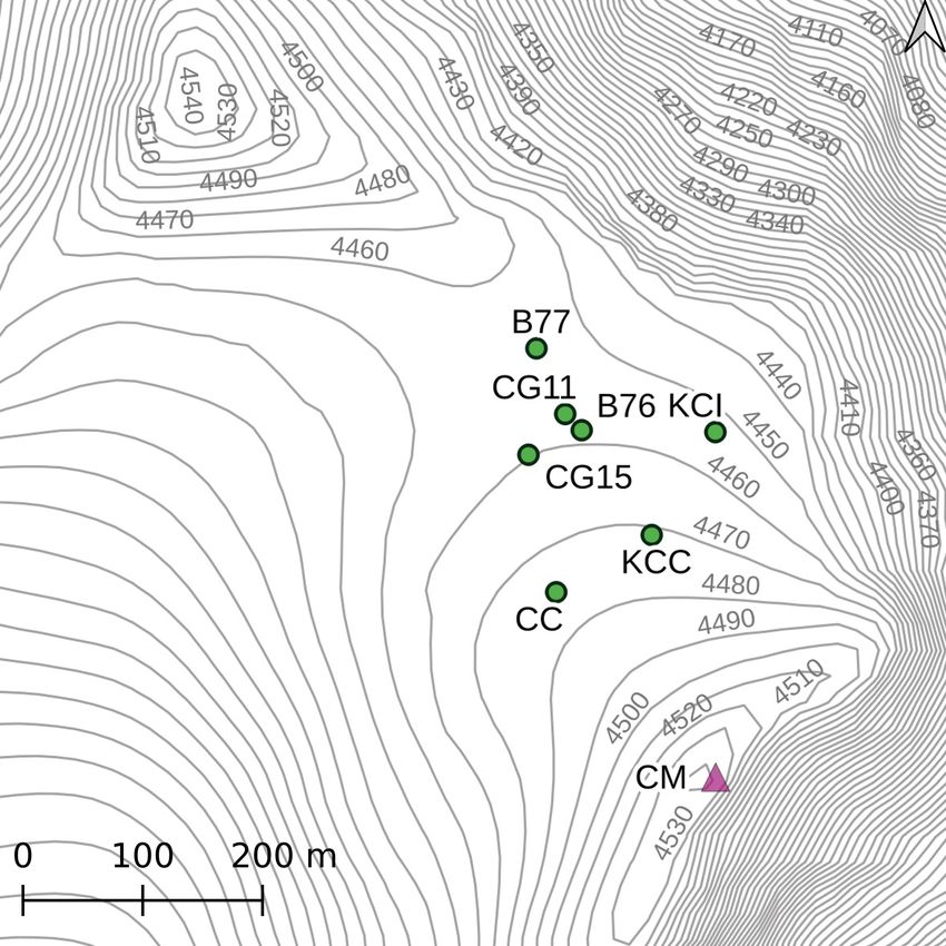
1032                                                        F. Banfi and C. De Michele: A local model of snow–firn dynamics

this task, models that integrate hydrological, nivological and      sion (single-layer) that models firn and underlying glacier ice
glaciological components and that consider a variable glacier       as a single layer. The latter consists of only six equations,
extension and the transient response of glaciers to climate         and it is therefore more suitable for a possible application
change are required (Luo et al., 2013).                             to a hydrological model. The former consists of four equa-
   Despite their importance, fully integrated glacio-               tions for the snowpack plus two equations for each firn layer.
hydrological catchment models are not common in the                 Providing a profile of density with depth, it captures better
literature (Wortmann et al., 2019). Some examples of                the influence of meteorological variables on snow and firn
glacio-hydrological models are provided by the works of             characteristics. Besides, it allows a better validation of the
Huss et al. (2010), Naz et al. (2014), Seibert et al. (2018)        snow–firn model. The equations that describe the snowpack
and Wortmann et al. (2019).                                         are derived from the work of De Michele et al. (2013) and
   Wortmann et al. (2019) grouped the main problems of              later Avanzi et al. (2015), modified in order to take into ac-
glacio-hydrological models into two categories: integration         count the contribution of wind erosion and the transforma-
and scale. With integration problems they refer to the simpli-      tion of snow into firn. To model the firn component, both the
fied or absent description of the remaining catchment hydrol-       densification model of Arnaud et al. (2000) and the one of
ogy in models that describe glacier processes in detail. The        Herron and Langway (1980) were implemented. In order to
decrease in the fraction of ice-covered areas requires a proper     test the model, a high-altitude site, Colle Gnifetti, belonging
description of both components, even in basins that are cur-        to the Monte Rosa massif, was chosen.
rently highly glacierized. Another aspect is the integration of        The paper is organized as follows: we present the model
nivological and glaciological components: a joint simulation        in Sect. 2, illustrate the case study in Sect. 3, give the results
of glacier mass balance and snow accumulation and melt is           in Sect. 4 and discuss them in Sect. 5. The conclusions are
required in order to avoid inconsistencies (Jost et al., 2012;      given in Sect. 6.
Naz et al., 2014). The problems of scale arise from the dif-
ferent resolutions required by glacial, nivological and hydro-
logical processes. Physically based models that consider all        2     Methodology
glacier processes (mass balance, subglacial drainage and ice
                                                                    In this section, firstly the snowpack model, proposed by
flow dynamics) are often too computationally expensive to be
                                                                    De Michele et al. (2013) and later modified by Avanzi et al.
used in a combined glacio-hydrological model that considers
                                                                    (2015) with the addition of the contribution of wind to snow
the entire catchment. In addition, they are characterized by a
                                                                    transport, is illustrated and secondly the model with the inte-
complexity higher than the one of many semi-distributed hy-
                                                                    gration of snow and firn processes is presented.
drological models. It is therefore necessary to develop glacier
models with a degree of complexity similar to the one of hy-        2.1    Snow model
drological models but that are still able to reproduce impor-
tant processes (Seibert et al., 2018).                              The snowpack is modelled, according to De Michele et al.
   In the present work, we give our contribution proposing          (2013) and Avanzi et al. (2015), as a mixture of dry and
a local model that follows the transformation of snow into          wet constituents. The solid deformable skeleton that con-
firn and glacier ice under the influence of meteorological          sists of both snow grains and pores has a total volume VS ,
variables (temperature, precipitation and wind speed). Exist-       unit area, height hS , mass MS and density ρS . The liquid
ing firn densification models are, in general, forced by snow       water inside the pores has a volume VW , unit area, height
characteristics. In this sense, the presented model allows us       hW , mass MW and constant density ρW = 1000 kg m−3 . The
to move the boundary of the firn densification models from          refrozen meltwater and rain inside the pores has a volume
surface accumulation and density to hourly meteorological           VMF with unit area, height hMF , mass MMF and constant den-
series. When we do not assume stationarity in the climate, in       sity ρi = 917 kg m−3 . It is also possible to define the bulk
fact, this is required to properly capture the effects of climate   snow density ρ, snow water equivalent SWE and volumetric
changes.                                                            liquid water content θW as ρ = (ρS hS + ρW hW + ρi hMF )/ h,
   The core of the model was derived from mass balance,             SWE = (ρh)/ρW and θW = hW / h, where h is the height of
momentum balance and rheological equations, governing the           the snowpack equal to h = hS + hhMF + hW − φhS i (Avanzi
evolution of snowpack and firn (depth and density of snow           et al., 2015) with φ being the porosity and hi denoting the
and firn, depth of water and refrozen meltwater and rain in-        Macaulay brackets that provide zero when the argument is
side the snowpack). The calculations of the terms in the re-        negative and its value when it is positive. The height h and
sulting equations were then approached looking at methods           hS always coincide except at the end of the snowpack exis-
already used in the literature; for example, snowmelt mass          tence when the liquid part and the solid part due to refreez-
flux was computed with a temperature-index approach and             ing become predominant (i.e. hMF +hW > φhS ). In this case,
the run-off from the snowpack with a flow matrix approach.          h > hS because a layer of water and/or ice forms on top of
We present two versions of the model: (1) a version (multi-         the deformable skeleton.
layer) that considers separately each firn layer and (2) a ver-

The Cryosphere, 16, 1031–1056, 2022                                                     https://doi.org/10.5194/tc-16-1031-2022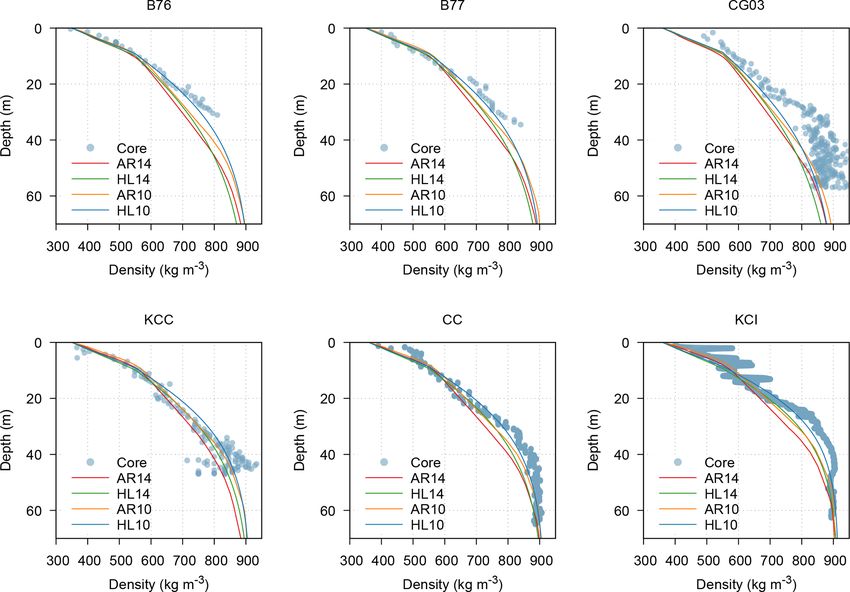
F. Banfi and C. De Michele: A local model of snow–firn dynamics                                                                 1033

   The model solves the mass balance for the dry and liquid
mass of the snowpack and the momentum balance and rheo-
logical equation for the solid deformable skeleton, resulting
in four ordinary differential equations (ODEs) with the vari-
ables hS , hW , hMF and ρS . The mass fluxes considered are (1)
solid precipitation events, snowmelt and wind erosion for the
dry-snow mass; (2) rain events, snowmelt, melt–freeze inside
the snowpack and run-off for the liquid mass; and (3) melt–
freeze for the mass of ice. The dry-snow density is obtained
considering (1) the compaction of snow due to compaction
not driven by wind, (2) the increase in the densification rate
due to drifting snow settlement and (3) densification due to
the addition of new mass. The following system is thus ob-
tained (see Appendix Sects. A1–A2 for the derivation of the
system and a detailed description of the terms in the equa-
tions):                                                            Figure 1. A column of snow, firn and ice as modelled by the single-
                                                                   layer (a) and multi-layer (b) version of the snow–firn model.
dhS    hS dρS ρNS                               Q
    =−        +       s − (I · a)(TA − Tτ ) − ,          (1a)
 dt    ρS dt       ρS                           ρS
dhW       ρS                                                       in accumulation with altitude in the Alps that occurs above
    =r+      (I · a)(TA − Tτ ) + (I ∗ · e · a)(TA − Tτ )           about 3500 m a.s.l. may be due to wind effects.
 dt      ρW
                                                                      In analogy with solid transport, snow is mobilized only
     − α · KW ,                                            (1b)    when wind velocity at the surface exceeds a given threshold
dhMF        ρW ∗                                                   that depends on physical properties of the surface snowpack
      =−        (I · e · a)(TA − Tτ ),                     (1c)
  dt        ρi                                                     (Li and Pomeroy, 1997). Once transport begins, snow can
dρS                                                                travel in two main modes: saltation and suspension (Déry and
     = (c · A1 · U )ρS exp(−B · (Tτ − TS ) − A2 · ρS )             Taylor, 1996; Pomeroy et al., 1997). The total snow transport
 dt
       ρNS − ρS                                                    Q is computed by the model with the following assumptions:
     +            s.                                       (1d)    (1) only snow erosion occurs, and no deposition of snow
           hS
                                                                   eroded in other positions is present; (2) measured wind speed
In Eq. (1a), ρNS is the density of fresh snow (kg m−3 ), s is      is always referred to a 10 m height – i.e. the height of the
the solid precipitation rate (m h−1 ), a is a calibration param-   snow on the ground is neglected; and (3) wind cannot erode
eter (m h−1 ◦ C−1 ), TA and Tτ are the air temperature and the     snow that has experienced a temperature greater than 0 ◦ C
threshold temperature for melting (◦ C), I is equal to hSh+k  S    for the presence of ice crusts or wet layers, following Vionnet
with k equal to 0.01 m if TA ≥ Tτ and zero otherwise (Avanzi       et al. (2018). These last two assumptions allow us to compute
et al., 2015), and Q is the mass of snow eroded by wind            the series of total snow transport Q decoupled from the snow
(kg m−2 h−1 ). In Eq. (1b), r is the liquid precipitation rate     model since knowledge of snow height is not required. In or-
(m h−1 ), e is a calibration parameter, I ∗ is equal to hW   hW    der to implement the routine, we followed, with some modi-
                                                              +k   fications, Lehning et al. (2000), where a model of snowdrift
                      hMF
if TA < Tτ and to hMF   +k if TA > Tτ (Avanzi et al., 2015),       was added to the one-dimensional snow model SNOWPACK
                  9 −1 −1
α = 1.9692 × 10 m h (DeWalle and Rango, 2008), and                 (further details about the implementation of the routine are
KW is the intrinsic permeability of water in snow (m2 ).           reported in Appendix Sect. A1).
In Eq. (1d), c = 0.10 · 3600 s h−1 , A1 = 0.0013 m−1 , A2 =
0.021 m3 kg−1 , B = 0.08 K−1 (Liston et al., 2007), U is the       2.2   Model of snow–firn dynamics
wind speed contribution (m s−1 ), and TS is the average snow
temperature (◦ C) obtained assuming thermal equilibrium be-        We propose here two versions of the snow–firn model. The
tween the constituents and a bilinear profile of temperature       first version (single-layer) models firn and underlying glacier
through depth (see De Michele et al., 2013, for further de-        ice as a single layer (Fig. 1, left panel). The resulting output
tails).                                                            is an average density and the total column height. The sec-
   With respect to the model by De Michele et al. (2013) and       ond version (multi-layer) considers separately each firn layer
Avanzi et al. (2015), the version presented in this work in-       (Fig. 1, right panel), and it allows us to distinguish between
cludes the contribution of wind erosion to mass balance and        layers of firn and glacier ice. The discretized profile of den-
effect of wind on densification. This is important when the        sity with depth can be obtained from this second implemen-
model is applied to high-altitude sites: Haeberli and Alean        tation. The snow layer is, instead, treated as a single layer in
(1985), in fact, suggested that a major part of the decrease       both versions.

https://doi.org/10.5194/tc-16-1031-2022                                                   The Cryosphere, 16, 1031–1056, 2022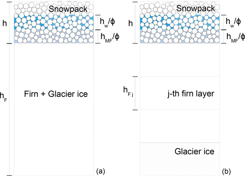
1034                                                        F. Banfi and C. De Michele: A local model of snow–firn dynamics

   In the model we neglected the amount of water percolation       ti is the time instant at the end of hydrological year i and δ(.)
inside firn. The presence of water inside firn varies greatly      is the Dirac delta function. In Eq. (2d), IF is equal to hFh+kF
                                                                                                                                   ,
depending on the type of glacier. At high altitudes, where         with k specified above if TA ≥ Tτ and equal to zero other-
maximum temperatures are rarely positive, the effects of per-      wise. In Eq. (2f), dρ  F
                                                                                        dt |comp is the densification of firn due to
colation due to melting are limited (Smiraglia et al., 2000);      compaction (see Sect. 2.4). Equations (2a)–(2f) are impulsive
at the cold site of Colle Gnifetti, where the model was ap-        differential equations (see e.g. Bainov and Simeonov, 1993,
plied, percolation occurs only in the few centimetres below        for mathematical details). This type of differential equation
the surface and does not involve previous-year layers (Alean       involving the impulse effect is used to describe the evolution
et al., 1983). If needed, the structure of the model allows us     of many physical phenomena that have a sudden change in
to easily implement additional processes.                          their states such as mechanical systems with impact; biolog-
   In order to separate snow from firn, we refer to firn’s orig-   ical systems such as heartbeats and blood flows; and popula-
inal definition, according to which firn is snow that has sur-     tion dynamics.
vived one melt season (Cuffey and Paterson, 2010).
                                                                   2.3   Multi-layer modelling of firn
2.2.1   One-layer modelling of firn
                                                                   Firn is modelled as a multi-layer column where each layer j
The model is composed of two layers: the snowpack (see             has volume VFj , unit area, height hFj , mass MFj and density
Sect. 2.1) and the column of firn below it. The firn is mod-       ρFj .
elled as a single impermeable layer of volume VF , unit area,        The equations of the model change as follows:
height hF , mass MF and density ρF (Fig. 1, left panel).
                                                                    dhS     hS dρS ρNS
   The model consists of six ODEs: the four equations of the            =−         +      s − (I · a)(TA − Tτ )
snow model and in addition the mass balance and momentum             dt     ρS dt     ρS
balance of firn. The mass variation in firn is obtained consid-           Q X
                                                                        −    −    hS δ(t − ti ),                               (3a)
ering firn melt, the effects of precipitation on firn and the             ρS    i
transformation of snow into firn at the end of each hydrolog-       dhW        ρS
ical year. The firn densification rate is obtained considering          =r+       (I · a)(TA − Tτ ) + (I ∗ · e · a)(TA − Tτ )
                                                                     dt        ρW
densification due to overburden stress and densification due                        X
to addition of new mass. The resulting system is thus as fol-           − α · KW −      hW δ(t − ti ),                        (3b)
lows (see Appendix A for the derivation of the system and a                               i
detailed description of the terms in the equations):                dhMF    ρW ∗                       X
                                                                         =−    (I · e · a)(TA − Tτ ) −   hMF δ(t − ti ), (3c)
dhS    hS dρS ρNS                              Q                     dt     ρi                         i
    =−         +       s − (I · a)(TA − Tτ ) −
 dt    ρS dt        ρS                         ρS                   dhF1     hF1 dρF1
      X                                                                  =−            − (IF · a)(TA − Tτ )δ(hS )
    −   hS δ(t − ti ),                                     (2a)      dt      ρF1 dt
         i                                                                 ρW                      X ρ
                                                                         +     rδ(hS )hTτ − TA i +         hδ(t − ti )
dhW        ρS                                                              ρF1                        ρF1
    =r+       (I · a)(TA − Tτ ) + (I ∗ · e · a)(TA − Tτ )                                           i
 dt        ρW
                                                                           X
                X                                                        −    hF1 δ(t − ti ),                                  (3d)
    − α · KW −      hW δ(t − ti ),                        (2b)                i
                    i                                               dhFj    hFj dρFj X
                                                                         =−           +       hFj −1 δ(t − ti )
dhMF       ρW ∗                       X                              dt     ρFj dt
        =−    (I · e · a)(TA − Tτ ) −   hMF δ(t − ti ), (2c)                                i
 dt        ρi                         i
                                                                           X
                                                                         −   hFj δ(t − ti ),                                   (3e)
dhF    hF dρF                                                                 i
    =−         − (IF · a)(TA − Tτ )δ(hS )
 dt    ρF dt                                                        dρS
      ρW                     Xρ                                          = (c · A1 · U )ρS exp(−B · (Tτ − TS ) − A2 · ρS )
    +    rδ(hS )hTτ − TA i +       hδ(t − ti ),            (2d)      dt
      ρF                      i
                                ρF                                         ρNS − ρS
                                                                        +             s,                                       (3f)
dρS                                                                            hS
    = (c · A1 · U )ρS exp(−B · (Tτ − TS ) − A2 · ρS )               dρF1    dρF1           X ρ − ρF1
 dt                                                                      =               +            hδ(t − ti ),             (3g)
      ρNS − ρS                                                       dt       dt comp        i
                                                                                                hF1
    +            s,                                        (2e)
          hS                                                        dρFj   dρFj
dρF   dρF           X ρ − ρF                                             =                ,                                    (3h)
    =             +           hδ(t − ti ).                  (2f)     dt     dt     comp
 dt    dt comp        i
                          hF
                                                                   where j goes from 2 to the total number of firn layers. Firn
The last terms in Eqs. (2a)–(2c) move, at the end of each melt     layers that reach the ice density or whose height goes to zero
season, the remaining snowpack (if present) in the firn layer;     are removed from the model.

The Cryosphere, 16, 1031–1056, 2022                                                    https://doi.org/10.5194/tc-16-1031-2022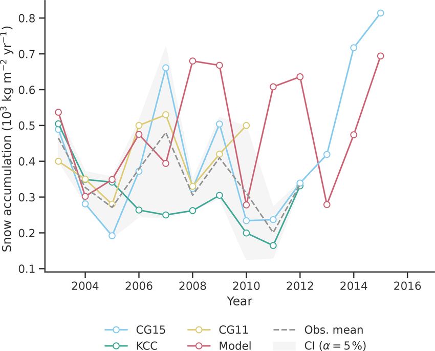
F. Banfi and C. De Michele: A local model of snow–firn dynamics 1035
2.4 Firn densification In the first stage (DD ≤ ρF /ρi ≤ D0), P is the over-
burden pressure (Pa) and γ = γ 0 exp − RG (TFQ 1
+273.15) in
The densification of firn due to compaction is usually sub- which RG is the gas constant, Q1 an activation energy
divided into three stages: (1) a first stage dominated by the equal to 48 × 103 J mol−1 , TF the average temperature of
settling of grains that allows us to reach densities of up to firn (◦ C), and γ 0 a parameter whose value is set in or-
about 550 kg m−3 , (2) a second stage dominated by sinter- der to have a continuous densification rate between the
ing that extends up to the close-off density (i.e. the den- first and second stage (estimated in Sect. 4.2). DD is
sity at which pores become isolated) of about 830 kg m−3 the relative surface density, and D0 is the relative den-
and (3) a last stage that ends when ice density is reached sity at the transition between the first stage and the sec-
in which further densification is driven by the compression ond stage.
In the second stage (D0 < ρF /ρi ≤ Dc ), A =
of the bubbles of air (Cuffey and Paterson, 2010). This last Q2
A0 exp − RG (TF +273.15) with A0 = 2.84 × 10⁻¹¹ Pa−3 h−1 ,
stage is in turn subdivided into two phases, depending on
ac is the average contact area, Z is the number of particle
if the pores are cylindrical or spherical. Different models of
contacts (see Appendix Sect. A3 for the expression of ac and
firn densification are available in the literature (see Lundin
Z) and Q2 is an activation energy. The value of Q2 was set
et al., 2017, for a review). Here we implemented the model
to 60 × 103 J mol−1 , as in the model of Arnaud et al. (2000),
of Arnaud et al. (2000) with some of the modifications pro-
since it is the typical activation energy associated with self-
posed by Bréant et al. (2017) (we will refer to it with the
diffusion of ice. However, at higher temperature (i.e. higher
abbreviation AR) and the model of Herron and Langway
than −10 ◦ C) a higher activation energy may be required to
(1980) (we will refer to it with the abbreviation HL). Other
best fit density profiles with firn densification models (Cuf-
models could also be implemented. Both HL and AR were
fey and Paterson, 2010; Arthern et al., 2010; Jacka and Jun,
developed for polar sites. The HL model was derived us-
1994). A discussion of the thermal variation in the creep
ing ice cores with a mean annual firn temperature between
parameter and the impact of the different sintering mecha-
−57 and −15 ◦ C and a mean annual accumulation between
nisms on it can be found in Bréant et al. (2017). Lastly, in the
0.022 × 10³ and 0.5 × 10³ kg m−2 yr−1 , while the AR model
third stage (ρF /ρi > Dc ), Pb is the pressure inside the bub-
was derived from cores with a mean annual firn temperature
bles equal to Pb = Pc (ρ F /ρi )(1−Dc )
Dc ·(1−ρF /ρi ) with Dc and Pc the rela-
between −57 and −19 ◦ C and a mean annual accumulation
tive density and pressure at the transition between the second
between 0.022×10³ and 1.1×10³ kg m−2 yr−1 . In the model
and third stage. In the single-layer version, the overburden
of AR, densification equations are based on grain sliding and
pressure P was computed as the overburden of the snowpack
creep deformations, even though they maintain empirical pa-
layer plus half of the firn layer. In the multi-layer version, we
rameters. The model of HL consists of empirical equations
computed the overburden for each layer of firn as the over-
tuned with ice cores, based on the assumption that a pro-
burden of the snowpack plus the overburden of all the firn
portionality is present between the variation in density and
layers above plus the overburden of half the firn layer con-
the variation in stress due to new accumulation. Besides, the
sidered.
model of AR represents stresses explicitly, while in HL the
In HL only the first and second densification stages are
load is parametrized through annual surface accumulation.
modelled. The equations are as follows:
The model of HL was already applied to non-polar ice
cores by Huss (2013), where the model was recalibrated dρF
in order to match depth–density profiles of temperate and =
dt comp
polythermal firn. In the presented application, the parame-
k0 · (ω × 103 ) · (ρi − ρF ) ρD ≤ ρF ≤ 550 kg m−3
ters were not recalibrated, despite the fact that the study site (5)
k1 · (ω × 103 )0.5 · (ρi − ρF ) 550 < ρF < 800 kg m−3
is an alpine site. This was motivated by the low mean an-
nual firn temperature (MAFT) and low surface accumulation
observed at Colle Gnifetti that resemble conditions of some where k0 = 11 exp − RG (T10
F
160
+273.15) , k1 =
polar sites. 575 exp − RG (T21 400
and ω is the annual snow ac-
F +273.15)
In AR all three stages of firn densification are modelled.
Equations are as follows: cumulation (kg m−2 yr−1 ). In HL the transition density
between the first and second stage is fixed and equal to
550 kg m−3 . In order to run the model of HL in a dynamic
dρF way, for each year we computed the annual accumulation
=
dt comp averaging the ones modelled between the year of deposition
of the firn layer and the year before the one considered,
,104 )
5 ρF
γ max(P
(ρ /ρ ) 2 1 + 0.5 6 − 3 ρi ρi DD ≤ ρF /ρi ≤ D0
F i
1/3 ac 1/2 4π·P ·ρi 3 following Stevens et al. (2020).
5.3A · (ρF /ρi )2 D0
ρi D0 < ρF /ρi ≤ Dc
π 3a ·Z·ρ
3 c F (4) Steady-state firn densification models are not applied to
ρF (1−ρF /ρi ) 2(P −Pb )
2A · ρi Dc < ρF /ρi ≤ 0.95 the superficial snow where the metamorphism is more com-
1 3
ρi (1−(1−ρF /ρi ) 3 )3
plex and significantly influenced by air temperature. The
9
4 A · (1 − ρF /ρi )(P − Pb )ρi ρF /ρi > 0.95.
https://doi.org/10.5194/tc-16-1031-2022 The Cryosphere, 16, 1031–1056, 2022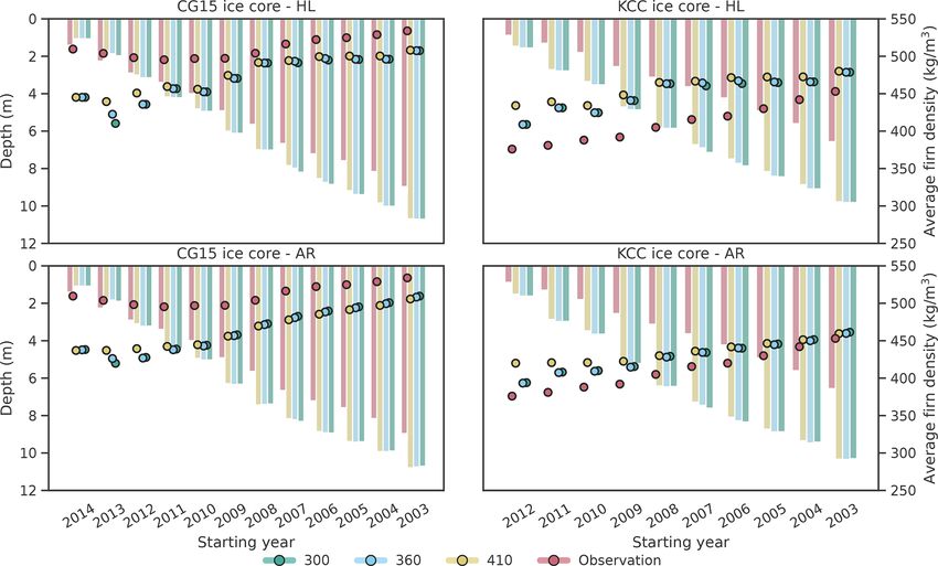
1036 F. Banfi and C. De Michele: A local model of snow–firn dynamics
original model of Arnaud et al. (2000), for example, was
used only for depths higher than 2 m. In this case, we ap-
plied them only to densities higher than a density ρD , which
represents the average snow density. For firn densities lower
than ρD , the densification equation of snow was adopted al-
though neglecting wind contribution. In this way, the tran-
sition between the two equations is driven by density rather
than associated with the end of a water year. This is impor-
tant, for example, when consistent fresh snow falls over the
snowpack at the end of the hydrological year.
2.4.1 Temperature profile
The energetic description of the volume was simplified as-
suming the constituents were in thermal equilibrium and as-
suming a bilinear profile of temperature through depth. Tem-
perature was assumed to vary linearly from the surface tem-
perature T0 to the MAFT at the depth zM at which seasonal
variation in temperature is negligible. Below zM , temperature
was kept constant and equal to MAFT. In cold glaciers the
value of MAFT is close to the mean annual air temperature
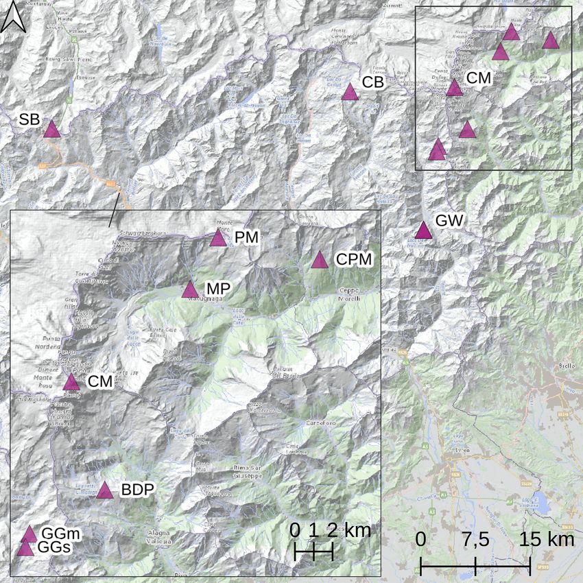
(MAAT) when meltwater percolation is limited (Suter et al., Figure 2. The site of Colle Gnifetti and the location of the ice cores
2001) while in temperate glaciers it is equal to the melting considered in the present work. CG03 and CG15 ice core share the
temperature (Cuffey and Paterson, 2010). Surface tempera- same location therefore CG03 is not shown. The position of Ca-
ture was fixed equal to TA if TA < 0 ◦ C and zero otherwise. panna Regina Margherita (CM) is also shown.
Huss (2013) has already assumed a bilinear profile of tem-
perature in order to study temperate firn densification, fixing
zM to 5 m since it is the typical penetration of winter air tem- gletscher (Border Glacier), and it forms a saddle that lies
perature. The temperature profile was then used to compute between the Signalkuppe (4554 m a.s.l.) and Zumsteinspitze
the average snow and firn temperatures that influence snow (4563 m a.s.l.) at an altitude of 4400–4550 m a.s.l. (Lüthi and
and firn densification. Funk, 2000) (Fig. 2). The glacier at Colle Gnifetti has a thick-
ness of between 60 and 120 m and a MAFT of −14 ◦ C (Wa-
2.5 Numerical model
genbach et al., 2012). The regime is that of a high-altitude
The model was solved using the forward Euler method with a site, i.e. nearly persistent sub-zero air temperature, a high
constant step size, 1t, of 1 h. To also compute the last terms precipitation total and high wind speed (Suter et al., 2001).
in Eqs. (1d), (2f) and (3g) when hS , hF and hF1 are zero, these A mean annual precipitation of 2.7 × 10³ kg m−2 yr−1 with
terms were calculated, following De Michele et al. (2013), as an interannual variability of 0.8 × 10³ kg m−2 yr−1 (Mariani
ρNS (t)−ρS ρ(t)−ρF h(t) ρ(t)−ρF1 h(t) et al., 2014) was estimated for the period 1961–1993 from
hS (t)+s(t)1t s(t), hF (t)+h(t) 1t and hF1 (t)+h(t) 1t . Regarding a core extracted at the upper Grenzgletscher (Eichler et al.,
the vertical discretization, the firn component of the multi- 2000).
layer version of the model was discretized modelling one Even though the site is characterized by high precip-
layer for each hydrological year. itation totals, accumulation in the saddle is considerably
lower and highly variable over the glacier surface due to
wind erosion, with values ranging from about 0.15 × 10³
3 Study area and data
to 1.2 × 10³ kg m−2 yr−1 depending on the wind exposure
In the following section we will present the study area (Alean et al., 1983; Lüthi and Funk, 2000; Licciulli et al.,
(Sect. 3.1), the data collection and handling (Sect. 3.2– 2020). Alean et al. (1983) measured the accumulation at CG
3.3), and finally the calibration and site-specific parameters between 17 August 1980 and 23 July 1982 with a network
(Sect. 3.4–3.5). of 30 stakes. For the period between 14 August 1981 and
23 July 1982 the mass balance was negative at all the stakes
3.1 Study area due to wind erosion, while the net accumulation of the hy-
drological year 1980–1981 varied between +0.04 × 10³ and
The site of Colle Gnifetti (CG) is part of the summit ranges +1.18 × 10³ kg m−2 yr−1 with the highest values on south-
of the Monte Rosa massif, Swiss–Italian Alps. It is the facing slopes. This occurs because the enhanced melting and
uppermost part of the accumulation area of the Grenz- refreezing cause the formation of wet layers and ice crusts
The Cryosphere, 16, 1031–1056, 2022 https://doi.org/10.5194/tc-16-1031-2022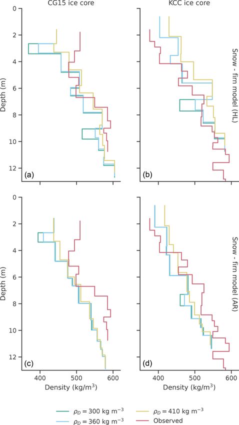
F. Banfi and C. De Michele: A local model of snow–firn dynamics                                                                    1037

and because higher temperatures are associated with faster
densification, and both these aspects reduce the possibility of
wind eroding snow. This also results in the fact that almost all
the snow that survives the melt season comes from summer
events (Bohleber et al., 2018; Schöner et al., 2002).

3.2   Data collection

The stations whose data were used in this study are pre-
sented in Fig. 3, and they are summarized in Table 1. Hourly
data of air temperature and wind speed at Capanna Regina
Margherita (CM, Margherita Hut in English) were used as
input for the model; hourly data at Passo del Moro (PM,
Monte Moro Pass in English) to reconstruct precipitation at
CM; and hourly and daily air temperature data at Macugnaga
Pecetto (MP), Passo del Moro, Bocchetta delle Pisse (BDP)
and Ceppo Morelli (CPM) to infill missing temperature data
at Capanna Regina Margherita. Hourly wind speed data at
Valtournenche–Cime Bianche (CB) and Col du Grand St
Bernard (SB, Great St Bernard Pass in English) were used to
infill missing wind speed data at CM. Hourly data at the me-
teorological stations of Gressoney-Saint-Jean – Weissmatten          Figure 3. Location of the meteorological stations used: Capanna
                                                                     Regina Margherita (CM), Macugnaga Pecetto (MP), Ceppo Morelli
(GWm) and Gressoney-la-Trinité – Gabiet (GGm) and snow
                                                                     (CPM), Passo del Moro (PM), Bocchetta delle Pisse (BDP), Col
water equivalent data (GWs and GGs) were used to calibrate           du Grand St Bernard (SB), Valtournenche–Cime Bianche (CB),
and validate the parameters a and e of the snow model. Snow          Gressoney-la-Trinité – Gabiet (GGm and GGs) and Gressoney-
water equivalent is measured by the Aosta Valley Region dur-         Saint-Jean – Weissmatten (GWm and GWs). The location of the
ing winter both at fixed locations and at itinerant sites. For       meteorological station at Weissmatten and the location of snow
GGs, 4 years of measurements was available with on aver-             measurements are only a few metres apart, so only one point is re-
age 24 data points for each winter. For GWs, 5 years was             ported (identified with GW). In the bottom left panel a zoom over
available with on average 8 data points for each winter.             some stations is included. All stations belong to Arpa Piemonte with
   The station of Capanna Regina Margherita, whose data              the exclusion of CB, GGm, GGs, GWm and GWs, which belong to
were used to run the snow–firn model, was installed in 2002          the Aosta Valley Region, and SB, which belongs to the National
by the Piedmont Region at the Regina Margherita Hut as part          Oceanic and Atmospheric Administration (NOAA). Source of the
                                                                     basemap: Arpa Piemonte geoportal.
of a project that aimed to study the interaction between syn-
optic flow and orography. With its 4560 m of altitude, it can
be considered the highest meteorological station in Europe,          Margherita, the MicroMet preprocessor (Liston and Elder,
and its wind speed series can be considered representative of        2006) was adopted for gaps smaller than 24 h and a long-
the synoptic conditions (Martorina et al., 2003). Due to its         term lapse rate approach with five stations (CM, MP, CPM,
recent installation, the use of these data limits the length of      PM, BDP) was adopted for longer gaps. MicroMet is a mete-
the simulation and the number of cores with which our re-            orological model that includes a data-fill procedure adopted
sults can be compared. Nevertheless, we believe that, given          here. The method distinguishes between three conditions: (1)
the peculiar characteristics of the station, the use of these data   for 1 h gaps the missing information is replaced with the
may give added value to this study.                                  average of the previous and next measurement; (2) for 2–
   In Table 2 ice core data are reported (Fig. 2). Available data    24 h gaps each missing value is replaced with the average of
consist of some or all of the following information: depth           the values recorded the next and previous day at the same
in metres, depth in metres of water equivalent, density and          hour; (3) for longer gaps an auto-regressive integrated mov-
dating. We recall that the first three variables are related, so     ing average (ARIMA) model is used (Hyndman and Athana-
one of them can be computed given the other two.                     sopoulos, 2021). Here, for the third condition, the long-term
                                                                     lapse rate approach was used, as specified above. In the pe-
3.3   Data handling                                                  riod 1 October 2002–13 August 2013, 0.37 % of hourly tem-
                                                                     perature data were missing. After the MicroMet procedure
The model requires as input a continuous series of air tem-          0.23 % remained missing and were substituted with a long-
perature, precipitation and wind speed.                              term lapse rate approach.
  Following the comparison presented by Henn et al.
(2013), to fill missing hourly temperature data at Capanna

https://doi.org/10.5194/tc-16-1031-2022                                                     The Cryosphere, 16, 1031–1056, 2022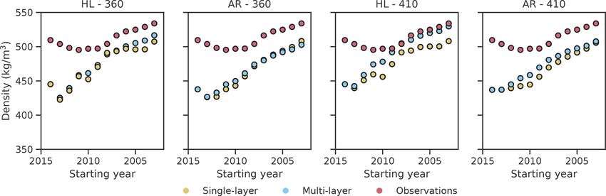
1038                                                           F. Banfi and C. De Michele: A local model of snow–firn dynamics

Table 1. Meteorological data employed in the case study (p stands for precipitation, SD for snow depth, TA for air temperature, u for average
wind speed and s for fresh snow). Hydrological years are identified by the last year; e.g. 2009 is hydrological year 2008–2009. With the term
hydrological year we refer to the period from 1 October to 30 September of the next year.

 Station name              Altitude     UTM x            UTM y      Variable         Aggregation     Period used               Source
                           (m a.s.l)   WGS84 (m)        WGS84 (m)
 Capanna Regina              4560        412930          5086564    TA , u           Hourly          1 October 2002–           Arpa
 Margherita (CM)                                                                                     13 August 2013            Piemonte
 Passo del Moro (PM)         2820        420739          5094227    TA               Daily           1 October 2002–           Arpa
                                                                                                     30 September 2007         Piemonte
 Passo del Moro (PM)         2820        420739          5094227    p, SD, TA , u,   Hourly          1 October 2002–           Arpa
                                                                                                     30 September 2019         Piemonte
 Bocchetta delle             2410        414709          5080807    TA               Daily           1 October 2002–           Arpa
 Pisse (BDP)                                                                                         30 September 2007         Piemonte
 Bocchetta delle             2410        414709          5080807    TA               Hourly          November 2002,            Arpa
 Pisse (BDP)                                                                                         September 2007            Piemonte
 Ceppo Morelli (CPM)         1995        426141          5093057    TA               Daily           1 October 2002–           Arpa
                                                                                                     30 September 2007         Piemonte
 Ceppo Morelli (CPM)         1995        426141          5093057    TA               Hourly          November 2002,            Arpa
                                                                                                     September 2007            Piemonte
 Gressoney-la-Trinité –      2379        410705          5078465    p, SD, TA , u    Hourly          1 October 2017–           Aosta Valley
 Gabiet (GGm)                                                                                        30 September 2021         Region
 Gressoney-la-Trinité –      2340        410490          5077754    SWE              Not fixed       Water years: 2018, 2019   Aosta Valley
 Gabiet (GGs)                                                                                        2020, 2021                Region
 Gressoney-Saint-Jean –      2038        408692          5066969    p, SD, TA , u    Hourly          1 October 2015–           Aosta Valley
 Weissmatten (GWm)                                                                                   30 September 2020         Region
 Gressoney-Saint-Jean –      2035        408686          5066982    SWE              Not fixed       Water years: 2016, 2017   Aosta Valley
 Weissmatten (GWs)                                                                                   2018, 2019, 2020          Region
 Valtournenche–              3100        398610          5085987    u                Hourly          1 October 2003–           Aosta Valley
 Cime Bianche (CB)                                                                                   30 September 2019         Region
 Col du Grand                2479        357703          5080871    u                Hourly          1 October 2002–           NOAA
 St Bernard (SB)                                                                                     30 September 2019

Table 2. Ice core data employed in the case study.

                               Name     Drilling date     Mean annual accumulation     Data source
                                                             (103 kg m−2 yr−1 )
                               B76      1976                        0.37               Gäggeler et al. (1983)
                               B77      1977                        0.32               Gäggeler et al. (1983)
                               CG03     2003                        0.45               Sigl et al. (2018)
                               CG15     2015                        0.45               Sigl et al. (2018)
                               CG11     2011                        0.41               Ardenghi (2012)
                               CC       1982                        0.22               Licciulli et al. (2020)
                               KCI      2005                        0.14               Licciulli et al. (2020)
                               KCC      2013                        0.22               Licciulli et al. (2020)

The Cryosphere, 16, 1031–1056, 2022                                                              https://doi.org/10.5194/tc-16-1031-2022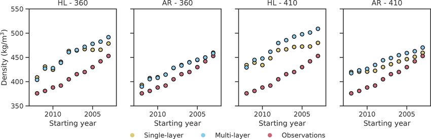
F. Banfi and C. De Michele: A local model of snow–firn dynamics                                                              1039

    Wind speed data measured at CM are characterized by re-        fore increased the resulting hourly solid precipitation with a
peated zero values that are not observed in nearby stations        constant factor in order to match the observed mean annual
and that are probably due to the freezing of the anemometer.       accumulation at CG of 2.7 × 10³ kg m−2 yr−1 . The total pre-
In the period 1 October 2002–13 August 2013 nearly 30 % of         cipitation series was then divided between solid and liquid
the wind speed data at CM were equal to zero, while 1.3 %          precipitation using a threshold of 1 ◦ C since this is the value
were missing. By comparison, in the same period, there were        generally found in Europe (Jennings et al., 2018).
2 % zero values in SB series. These zero values were there-
fore considered missing. To fill missing wind speed data at        3.4   Calibration of model’s parameters
CM, the MicroMet procedure was used for gaps smaller than
24 h. For gaps longer than 24 h, data were replaced using          The model requires the calibration of three parameters,
measurements at CB or, if wind speed data were also missing        namely a and e in Eqs. (1a)–(1c) and γ 0 in Eq. (4).
at CB, with data measured at SB. In both series, zero wind            The parameters a and e were calibrated running the snow
speed values recorded for more than 4 consecutive hours            model, with the addition of the wind module, at Gressoney-
were set as missing. In order to take into account the different   Saint-Jean – Weissmatten, with an hourly time step from
characteristics of the sites, we first computed for each of the    1 October 2015 to 30 September 2020. Input series were
three stations the mean and standard deviation for each hour       processed as reported for PM in Sect. 3.3. The parameter
of the year, and we removed this from the data. Missing data       a governs the amount of snowmelt and consequently snow
at CM were first replaced with the corresponding residual          height and the relative amount of snow and ice inside the
value measured at CB (or SB), and then the final value was         snowpack, thus influencing snow water equivalent and den-
obtained using the mean and standard deviation estimated at        sity. On the contrary, the parameter e influences only the
CM. Reconstructed negative wind speed values at CM were            relative amount of snow and ice inside the snowpack and
set to zero. Missing wind speed data at CM were set to zero        does not contribute to snow height. The calibration problem
if they were zero at CB (or SB).                                   is therefore a multi-objective one, since we could optimize
    The precipitation series at CM was reconstructed using         the error in both snow height and density or SWE. We de-
hourly data measured at PM. The station was chosen due to          cided to move from a multi-objective to a single-objective
it being in the vicinity of CM and its altitude of 2820 m a.s.l.   optimization problem, aggregating the NSE (Nash–Sutcliffe
Using the formula proposed by Alpert (1986) and consider-          efficiency) between observed and simulated snow depth data
ing a bell-shaped mountain, we estimated for the Monte Rosa        and the NSE between observed and simulated snow water
massif an altitude of maximum precipitation of zm = 2547 m.        equivalent data. We calculated the error metrics considering
The altitude of maximum precipitation is away from the crest       together all the available years but computing the measure
as is typical of large mountains (Roe, 2005). We therefore ex-     only in the periods with snow depth higher than zero, and we
pect to have similar precipitation totals at CM and PM. The        aggregated them, giving a weight of 0.7 to the first and 0.3
precipitation series measured at PM needs to be integrated         to the second. In this way we took into account the higher
with snow depth data due to the under-catch of solid precip-       uncertainty in SWE data due to the shorter sample length
itation by the pluviometer or does not catch solid precipita-      and the non-coincidence between the location of the meteo-
tion events in winter. In order to reconstruct the total precip-   rological station and the snow measurements. The optimum
itation series, we followed the routine presented by Avanzi        parameters were then estimated for different moving-average
et al. (2014). Solid precipitation is obtained looking at the      windows, used to process solid precipitation input data, with
positive variations in snow depth data, while rainfall is given    the use of a population-evolution-based algorithm, namely
by the difference, if positive, between total precipitation and    SCE-UA (Shuffled Complex Evolution – University of Ari-
solid precipitation. Positive variations in snow depth, how-       zona) (Duan et al., 1992, 1993). We thus obtained a pair of
ever, may also be recorded when strong temperature vari-           a and e values for each window, and we selected the one
ations occur, thus introducing false events. Unlike Avanzi         maximizing the objective function. The validation was per-
et al. (2014), we approached this problem smoothing the            formed applying the model with the selected set of parame-
snow depth series with a moving average whose window size          ters at Gressoney-la-Trinité – Gabiet for the period 1 Octo-
was calibrated running the snow model at PM and looking for        ber 2017–30 September 2021.
the best match between simulations and observations. Even             The parameter γ 0 , which governs the firn densification rate
though PM has an altitude higher than the estimated altitude       in AR, was chosen in order to have a continuous densifi-
of maximum precipitation, we obtained a mean annual pre-           cation rate between the first and second stage of densifica-
cipitation of about 2 × 10³ kg m−2 yr−1 for the period 2002–       tion. For each of the available ice cores, with the exception
2019, lower than the one estimated at CG by Mariani et al.         of CG11, we computed the parameter γ 0 running AR in a
(2014). We suppose this may be due to wind erosion events;         steady-state condition (Bader, 1954) using the mean accu-
the procedure implemented by Avanzi et al. (2014), in fact,        mulation reported in Table 2. In addition, the parameters of
may compensate for snow depth variations due to wind ero-          the firn densification model chosen may need calibration if
sion decreasing the estimated solid precipitation. We there-       applied to sites significantly different from the polar ones.

https://doi.org/10.5194/tc-16-1031-2022                                                 The Cryosphere, 16, 1031–1056, 2022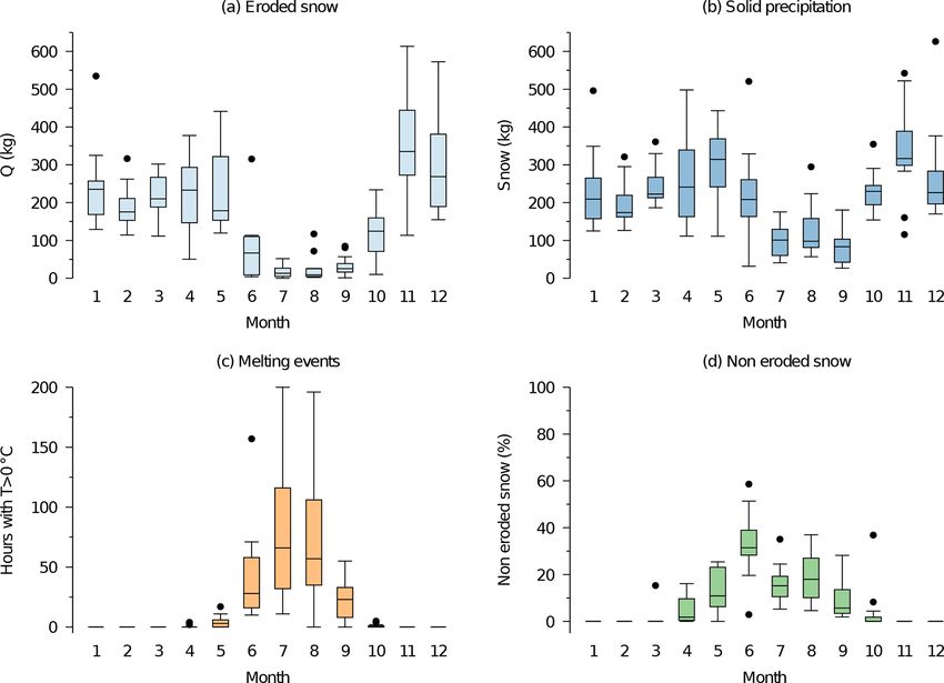
1040                                                        F. Banfi and C. De Michele: A local model of snow–firn dynamics

3.5    Site-specific parameters                                    Table 3. Modelled and observed mean (µ) and standard deviation
                                                                   (σ ) of the accumulation rate for the period 2003–2010.
In order to apply AR we use D0 = 0.56 (Bréant et al., 2017),
Pc = 740×102 Pa (Lüthi and Funk, 2000) and Dc = 0.9 since                          µ (103 kg m−2 yr−1 )   σ (103 kg m−2 yr−1 )
the precise value is not known at CG (Lüthi and Funk,
                                                                           Model            0.49                 0.15
2000). Two different firn temperatures, TF = −14 ◦ C and
                                                                           CG11             0.41                 0.09
TF = −10 ◦ C, that cover the observed ice temperatures at                  KCC              0.31                 0.09
CG (Lüthi and Funk, 2000) were tested together with dif-                   CG15             0.38                 0.16
ferent surface densities, chosen looking at values already
used in the literature at CG. We selected three values: ρD =
300 kg m−3 , ρD = 360 kg m−3 and ρD = 410 kg m−3 , the val-
ues already assumed by Licciulli et al. (2020) and Lüthi and       very good performances when applied to the KCC ice core.
Funk (2000). The model of AR was run with a slight mod-            The worst performances occur for CG03 with an underesti-
ification. We used the first-stage densification equation up       mation of the densification rate for all depths. For the remain-
to a relative density of 0.6, but we kept D0 = 0.56 in the         ing ice cores the models of AR and HL have a good fit up to
second-stage densification equation. The latter, in fact, can-     depths of about 20–30 m, but they underestimate the densi-
not be applied for D = D0 , and it gives densification rates       fication rate below it. The profiles show in general a better
tending to infinity for values tending to D0 . The other site-     performance of HL. We recall that the model of HL was de-
specific parameters of the snow–firn model that require spec-      rived also considering cores with MAFT and accumulation
ification are zM , set to 5 m (Haeberli and Funk, 1991), and the   close to the ones of CG, while AR was optimized for cores
grain radius R, which influences the threshold wind speed.         with lower MAFT.
It is defined as R = 3/(ρi SSA), where SSA is the specific
                                                                   4.3     Snow accumulation
surface area in m2 kg−1 . SSA was computed adopting the
parametrization of Domine et al. (2007) for recent snow:
                                                                   The annual accumulation obtained from the snow–firn model
SSA = −16.051 ln(ρS × 10−3 ) + 7.01.
                                                                   is reported in Fig. 5, along with the values retrieved from the
                                                                   three available ice cores, the average value of the observa-
4     Results                                                      tions and its 95 % confidence interval. The RMSE between
                                                                   the model and the average of the observations is equal to
4.1    Parameters’ estimation                                      0.22×10³ kg m−2 yr−1 , and the modelled and observed aver-
                                                                   age annual accumulation and standard deviation are reported
We obtained a value of the parameters a and e of 2.94 ×            in Table 3.
10−4 m h−1 ◦ C−1 and 0.164, respectively. The combined                In order to better understand the characteristics of the ac-
NSE in calibration is 0.82, with a NSE of 0.84 and 0.78 for        cumulation at CG, the monthly box plots of snow transport;
snow depth and snow water equivalent data, respectively. In        solid precipitation; number of hours with TA > 0 ◦ C, which
validation, the combined NSE and the NSE values for snow           in the model correspond to hours with melting; and monthly
depth and snow water equivalent are 0.77, 0.84 and 0.61,           contribution to annual accumulation, computed for each
respectively. We also computed the RMSE and mean bias              month as 100 × (solid precipitation − eroded snow) / solid
error (MBE) in validation, which are equal to 0.126 × 10³          precipitation, are provided in Fig. 6. Since snow is moved
and 0.0116 × 10³ kg m−2 yr−1 for snow water equivalent and         into firn at the end of September and wind is not allowed to
0.26 and 0.0672 m for snow depth. Avanzi et al. (2014) es-         erode firn, the fraction of conserved snow of September may
timated the parameter a for a selection of 40 sites with al-       be overestimated and the snow transport of October underes-
titudes between 91 and 3389 m a.s.l. within the SNOTEL             timated. We can see that annual accumulation is composed of
(Snow Telemetry) network, a network of automated stations          snow deposited mainly between April and September, with
located in mountain basins of the western USA and oper-            June the month that on average contributes the most. The
ated by the Natural Resources Conservation Service (NRCS).         months in which solid precipitation is conserved are also the
They obtained median values of a of between 1 × 10⁻⁴ and           months in which temperature goes above the melting point;
6 × 10⁻⁴ m h−1 ◦ C−1 . Regarding the parameter e, values of        winter snow, instead, is completely removed.
0.2 and 0.25 were estimated by Avanzi et al. (2015) for two
sites in Japan.                                                    4.4     Firn density

4.2    Steady-state firn densification                             4.4.1    One-layer model version

The depth–density profiles obtained using the model of AR          The modelled firn density was compared with the density
and HL in a steady-state condition are reported in Fig. 4 for      estimated from KCC and CG15 ice cores. With the one-
a surface density ρD = 360 kg m−3 . Both HL and AR have            layer version, we obtain one average value of firn density

The Cryosphere, 16, 1031–1056, 2022                                                       https://doi.org/10.5194/tc-16-1031-2022
F. Banfi and C. De Michele: A local model of snow–firn dynamics 1041
Figure 4. Observed and modelled depth–density profiles. Modelled profiles are obtained running Arnaud et al. (2000) (AR) and Herron and
Langway (1980) (HL) in a steady-state condition. The numbers 14 and 10 stand for a mean annual firn temperature of −14 and −10 ◦ C,
respectively.
For KCC we fixed the MAFT to −14 ◦ C, while for CG15 we
fixed it to −10 ◦ C, looking for the best performance in Fig. 4.
Regarding firn density, we have contrasting results de-
pending on the core and the densification model adopted.
Both model versions overestimate KCC density with a bet-
ter performance when AR is implemented; on the contrary
we obtained an underestimation of CG15 average density,
with a better performance when HL is implemented. In all
the combinations, however, we observed a reduction in the
error when more firn layers are averaged.
Moving to firn depth, the model nearly always predicts
higher depths, with more significant differences for the KCC
ice core.
4.4.2 Multi-layer model version
Figure 5. Annual accumulation modelled and retrieved from three
ice cores. The average of the annual accumulations from ice cores The modelled density profile was compared with KCC and
and its 95 % confidence interval are also reported. CG15 density data, implementing in the model both AR
and HL (Fig. 8) and testing three different transition den-
sities between snow and firn. Profiles are reported as steps,
where each step corresponds to a firn layer. Focusing on the
for each run of the model. We therefore run the model mul- CG15 ice core, we modelled, with both versions, lower den-
tiple times, fixing the end year of the simulation to the date sities in the first 4–5 m, with a layer with a particularly low
of the core drilling and anticipating at each run the starting density not matched by the ice core data at around 1–2 m
date of 1 year. For each run, the corresponding observed firn from the surface. This marked decrease however is reduced
density was obtained averaging the density profile of the ice when a ρD of 410 kg m−3 is chosen. For higher depths, the
core associated with the same range of years. The results ob- model with AR implemented underestimates CG15 density,
tained implementing both AR and HL are reported in Fig. 7. while with HL a better match of the profile is observed. The
https://doi.org/10.5194/tc-16-1031-2022 The Cryosphere, 16, 1031–1056, 20221042 F. Banfi and C. De Michele: A local model of snow–firn dynamics Figure 6. Box plots of monthly eroded snow (a), monthly solid precipitation (b), monthly number of hours with above-zero temperatures (c) and monthly fraction of conserved solid precipitation (d), obtained for the period 1 October 2002–30 September 2015. The horizontal bar inside the box is drawn at the median, and the upper and lower ends of the box are drawn at the upper and lower quartile, respectively. The vertical lines, called whiskers, extend up to the most distant point that has a value within 1.5 times the interquartile range. The points outside these limits are drawn individually with dots. Figure 7. Observed and modelled (with one-layer version) average firn density (dots, right axis) and depth (bars, left axis) for KCC and CG15. Each cluster corresponds to a run of the model whose starting date is reported on the x axis. The ending year for all runs is 30 August 2013 for KCC and 30 September 2015 for CG15. AR and HL stand for the model versions with Arnaud et al. (2000) and Herron and Langway (1980) implemented, respectively. The values 300, 360 and 410 stand for the chosen value of ρD . The Cryosphere, 16, 1031–1056, 2022 https://doi.org/10.5194/tc-16-1031-2022
F. Banfi and C. De Michele: A local model of snow–firn dynamics                                                              1043

                                                                   we compare in Figs. 9–10 the average firn density obtained
                                                                   with the single-layer version of the model or averaging the
                                                                   density of each individual firn layer obtained with the multi-
                                                                   layer version, weighted for their heights. The results for ρD =
                                                                   300 kg m−3 are not reported since they were not significantly
                                                                   different from the ones with ρD = 360 kg m−3 . Setting ρD to
                                                                   360 kg m−3 , we have, implementing HL, a maximum differ-
                                                                   ence between the two average densities of 16.7 kg m−3 , ob-
                                                                   tained for the KCC ice core, and, implementing AR, a maxi-
                                                                   mum difference of 7 kg m−3 , obtained for the CG15 ice core.
                                                                   Higher differences are obtained moving to ρD = 410 kg m−3 ,
                                                                   with a maximum difference of 29 and 14 kg m−3 implement-
                                                                   ing HL and AR, respectively, obtained for the KCC ice core.
                                                                   In all cases the multi-layer version predicts higher average
                                                                   densities.

                                                                   5     Discussion

                                                                   5.1    Steady-state firn densification

                                                                   Figure 4 shows a variable performance of the firn densifica-
                                                                   tion model depending on the ice core considered; with the
                                                                   exception of KCC and CG15, which show a very good and
                                                                   a very poor performance, respectively, for all the other cores
                                                                   we have a good fit up to a density of about 600–700 kg m−3 .
                                                                   Bréant et al. (2017), who modified the original model of AR,
                                                                   also observed a variable agreement between the data and
                                                                   model, also for sites with similar accumulation and temper-
                                                                   ature. They suggested that this may be due to different flow
                                                                   regimes of the sites, since their 1D model does not include
                                                                   this effect. Another consideration that emerges from Fig. 4,
                                                                   also pointed out by Bréant et al. (2017), is that the modelled
                                                                   profile results in worse performances when the observed den-
                                                                   sity profile does not show a clear change in the densification
                                                                   rate near the critical density D0 . The transition is, in fact,
                                                                   more evident for the KCC ice core, which is associated with
Figure 8. Observed and modelled (with multi-layer version) firn    the best fit. Finally, Bréant et al. (2017) reported a tendency
density profiles for KCC (b, d) and CG15 (a, c). AR and HL stand
                                                                   of the model to overestimate the densification rate for lower
for the model versions with Arnaud et al. (2000) and Herron and
                                                                   densities and to underestimate it for higher densities. This
Langway (1980) implemented, respectively.
                                                                   is coherent with the results obtained, in which HL predicts
                                                                   lower densities before D0 and higher densities after D0 if
                                                                   compared with AR. In order to compare modelled and ob-
best performance is obtained implementing HL and selecting         served profiles in Fig. 4, it is important to point out that the
ρD = 410 kg m−3 , with a mismatch only in the first metres.        two models assume stationary conditions; therefore they are
   Moving to the KCC ice core, the model with AR imple-            not able to reproduce possible changes in the glaciological
mented results in an overestimation of density up to a depth       characteristics. In some of the ice cores it is possible to see
of around 4 m and an underestimation below it. Implement-          a bend in the profile in correspondence to about 20–30 m.
ing HL, the density is instead overestimated except for a layer    The reason could be a combination of ice flow and the up-
at around 8 m of depth.                                            stream effect, i.e. changes in snow accumulation upstream,
                                                                   and these effects cannot be reproduced by a 1D model like
4.5   Comparison between multi- and single-layer model             the ones used.
      versions

In order to understand the approximation introduced mod-
elling firn as a single layer instead of a multi-layer column,

https://doi.org/10.5194/tc-16-1031-2022                                                 The Cryosphere, 16, 1031–1056, 2022
You can also read