How well are we able to close the water budget at the global scale?
←
→
Page content transcription
If your browser does not render page correctly, please read the page content below
Hydrol. Earth Syst. Sci., 26, 35–54, 2022
https://doi.org/10.5194/hess-26-35-2022
© Author(s) 2022. This work is distributed under
the Creative Commons Attribution 4.0 License.

How well are we able to close the water budget at the global scale?
Fanny Lehmann1 , Bramha Dutt Vishwakarma1,2 , and Jonathan Bamber1,3
1 Schoolof Geographical Sciences, University of Bristol, UK
2 Interdisciplinary
                 Centre for Water Research, Indian Institute of Science, Bengaluru, India
3 Department of Aerospace and Geodesy, Data Science in Earth Observation,

Technical University of Munich, Munich, Germany

Correspondence: Fanny Lehmann (fanny.lehmann@bristol.ac.uk)

Received: 25 May 2021 – Discussion started: 28 June 2021
Revised: 12 October 2021 – Accepted: 20 November 2021 – Published: 4 January 2022

Abstract. The water budget equation describes the exchange        gions based on, for example, climatic zone. We identified that
of water between the land, ocean, and atmosphere. Being           some of the good results were obtained due to the cancella-
able to adequately close the water budget gives confidence        tion of errors in poor estimates of water budget components.
in our ability to model and/or observe the spatio-temporal        Therefore, we used coefficients of variation to determine the
variations in the water cycle and its components. Due to ad-      relative quality of a data product, which helped us to iden-
vances in observation techniques, satellite sensors, and mod-     tify bad combinations giving us good results. In general, wa-
elling, a number of data products are available that represent    ter budget components from ERA5-Land and the Catchment
the components of water budget in both space and time. De-        Land Surface Model (CLSM) performed better than other
spite these advances, closure of the water budget at the global   products for most climatic zones. Conversely, the latest ver-
scale has been elusive.                                           sion of CLSM, v2.2, performed poorly for evapotranspira-
   In this study, we attempt to close the global water bud-       tion in snow-dominated catchments compared, for example,
get using precipitation, evapotranspiration, and runoff data      with its predecessor and other datasets available. Thus, the
at the catchment scale. The large number of recent state-         nature of the catchment dynamics and balance between com-
of-the-art datasets provides a new evaluation of well-used        ponents affects the optimum combination of datasets. For re-
datasets. These estimates are compared to terrestrial water       gional studies, the combination of datasets that provides the
storage (TWS) changes as measured by the Gravity Recov-           most realistic TWS for a basin will depend on its climatic
ery And Climate Experiment (GRACE) satellite mission. We          conditions and factors that cannot be determined a priori. We
investigated 189 river basins covering more than 90 % of the      believe that the results of this study provide a road map for
continental land area. TWS changes derived from the water         studying the water budget at catchment scale.
balance equation were compared against GRACE data us-
ing two metrics: the Nash–Sutcliffe efficiency (NSE) and the
cyclostationary NSE. These metrics were used to assess the
performance of more than 1600 combinations of the various
datasets considered.                                              1   Introduction
   We found a positive NSE and cyclostationary NSE in
99 % and 62 % of the basins examined respectively. This           A better understanding of hydrological processes at the
means that TWS changes reconstructed from the water bal-          catchment scale has been highlighted as one of the key chal-
ance equation were more accurate than the long-term (NSE)         lenges for hydrologists in the 21st century (Blöschl et al.,
and monthly (cyclostationary NSE) mean of GRACE time              2019). One of the key processes is the terrestrial water cycle
series in the corresponding basins. By analysing different        which can be described by the water balance equation:
combinations of the datasets that make up the water balance,
we identified data products that performed well in certain re-    dTWS
                                                                       = P − ET − R.                                         (1)
                                                                    dt

Published by Copernicus Publications on behalf of the European Geosciences Union.
36                                    F. Lehmann et al.: How well are we able to close the water budget at the global scale?

This equation expresses the total amount of water gained by         trial water cycle components (Rodell et al., 2015). The water
a river catchment in the form of precipitation (P ) as the sum      balance equation has been used to compensate for this lack
of water returning back to the atmosphere through evapo-            of knowledge and increase our understanding of ET. Water
transpiration (ET), water flowing out of the catchment in the       budget studies have generally found that ET inferred from
form of runoff (R), and any changes in the terrestrial water        the water balance equation agrees well with remote sensing
storage (TWS). TWS is defined as the sum of water stored as         estimates in terms of seasonal cycle but presents larger inter-
snow, canopy, soil moisture, groundwater, and surface water         annual variability (Liu et al., 2016; Pascolini-Campbell et al.,
(Scanlon et al., 2018). The water balance equation is a bud-        2020; Swann and Koven, 2017) and larger magnitudes (Bhat-
get equation that follows the conservation of mass, and it is       tarai et al., 2019; Long et al., 2014; Wan et al., 2015).
an indispensable tool for validating our understanding of the          Apart from ET, our knowledge of R also benefits from
catchment-scale water cycle.                                        water budget estimations. Although river discharge can be
   Several studies have used the water balance equation to ex-      measured by gauges, the spatio-temporal coverage of in situ
plain the hydro-climatic changes experienced in a river catch-      measurements is limited due to a lack of resources in some
ment (e.g. Landerer et al., 2010; Pan et al., 2012; Oliveira        regions and political will to share data. Uncertainties and bi-
et al., 2014; Saemian et al., 2020), to validate modelled es-       ases in P have been found to be the main drivers of the inac-
timates of one component (e.g. Bhattarai et al., 2019; Long         curacy in budget-inferred R (Sheffield et al., 2009; Oliveira
et al., 2015; Wan et al., 2015), or to estimate one component       et al., 2014; Sneeuw et al., 2014; Wang et al., 2014; Xie et al.,
when others are known (Chen et al., 2020; Gao et al., 2010;         2019). Water budget studies using R as a reference variable
Wang et al., 2014). It should be noted, however, that the ac-       also point out the difficulty involved in finding datasets able
curacy of the result in these studies is limited by uncertainties   to close the water budget (Chen et al., 2020; Gao et al., 2010;
associated with individual components. For example, Sahoo           Lorenz et al., 2014). Moreover, ET and R are strongly in-
et al. (2011) attempted to close the water balance equation         tertwined, and accurate estimates of one cannot be achieved
for 10 large catchments and found that the imbalance error          without a better constraint on the other (Armanios and Fisher,
amounted to up to 25 % of mean annual precipitation. Ad-            2014; Lv et al., 2017; Penatti et al., 2015).
ditionally, Zhang et al. (2018) highlighted the source of the          To improve the reliability of available data, the water bud-
imbalance error as being predominantly from stark disagree-         get can be used as a discriminating tool to assess the accu-
ment between evapotranspiration estimates.                          racy of various datasets. For this to be achieved, there is a
   Obtaining high-quality spatio-temporal estimates of com-         need to first evaluate the water budget closure globally, in-
ponents of the water balance is challenging due to a lack           cluding basins of all sizes and comparing as many state-of-
of global in situ measurement networks and political will           the-art datasets as possible. This review is currently lacking
to sustain any existing network. Therefore, the era of satel-       because a majority of studies have concentrated only on a
lite remote sensing offers an excellent solution to monitoring      few selected basins with specific climatic conditions (e.g. the
the hydrosphere. With the help of dedicated satellite mis-          Amazon Basin – Swann and Koven, 2017; Chen et al., 2020)
sions, we are able to measure variables that can be used            or basins highly impacted by human activities (e.g. the Yel-
to estimate water balance components. However, monitor-             low River basin – Lv et al., 2017; Long et al., 2015). Ad-
ing TWS has been the most difficult part because it includes        ditionally, the studies that look at several basins worldwide
water on and below the surface of the Earth, and optical re-        have only evaluated sparsely distributed basins, which leaves
mote sensing can only offer information near the surface.           entire zones without analysis (Sahoo et al., 2011; Pan et al.,
This issue was solved by the launch of the Gravity Recovery         2012; Lorenz et al., 2014; Liu et al., 2016; Zhang et al.,
And Climate Experiment (GRACE) satellite gravimetry mis-            2018). This has deprived hydrologists of a comprehensive
sion from the German GeoForschungsZentrum (GFZ) and                 global overview of the water budget.
the National Aeronautics and Space Administration (NASA)               Returning to the requirement for basins of all sizes, basins
in 2002 (Wahr et al., 1998; Tapley, 2004). This mission mea-        were also generally chosen to be quite large in the majority
sures the temporal variations in the Earth’s gravity field,         of studies. It is known that the accuracy of GRACE measure-
which can then be related to water mass change on and below         ments is directly proportional to the size of the basin (Rodell
the surface of the Earth. GRACE provides the most accurate          and Famiglietti, 1999; Wahr et al., 2006; Vishwakarma et al.,
global estimations of TWS to date, which can be used in the         2018); however, the lower limit of ∼ 200 000 km2 established
water balance equation (Eq. 1).                                     by Longuevergne et al. (2010), which has long been used, is
   Another challenge concerns components like ET with a             no longer a requirement to retrieve GRACE signals. It has
high spatial variability, which requires precise satellite esti-    been shown that basins as small as ∼ 70 000 km2 can be pre-
mates that are not consistently available due to observational      cisely recovered by GRACE measurements and that their size
constraints (Fisher et al., 2017). As ET accounts for up to         do not influence the closure of the water budget (Gao et al.,
60 % of precipitation in some regions, it is a crucial com-         2010; Lorenz et al., 2014; Vishwakarma et al., 2018). There-
ponent of the water cycle (Oki and Kanae, 2006). It also            fore, they are included in the current study.
constitutes the most significant uncertainties of the terres-

Hydrol. Earth Syst. Sci., 26, 35–54, 2022                                               https://doi.org/10.5194/hess-26-35-2022
F. Lehmann et al.: How well are we able to close the water budget at the global scale? 37
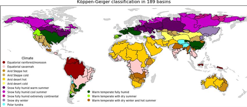
Figure 1. The 189 basins larger than 63 000 km2 with their corresponding climate zone.
Regarding the number of datasets to be examined, each 2.2 Datasets
water budget study uses different datasets, some of which
were available only over a given continent or over short We have used freely available global state-of-the-art datasets
time periods. To the authors’ best knowledge, Lorenz et al. with a temporal resolution smaller than or equal to 1 month
(2014) conducted the study comparing the largest number and coverage of at least 2003 to 2014. If necessary, data
of datasets by assessing more than 180 combinations of P , have been interpolated to 0.5◦ × 0.5◦ grids using bilinear in-
ET, and TWS datasets. However, many datasets have since terpolation to correspond with monthly TWS derived from
improved, especially reanalyses such as ERA-Interim (Dee the GRACE satellite mission. In this study, GRACE mas-
et al., 2011) and MERRA-Land (Reichle et al., 2011). It con fields were obtained from the Jet Propulsion Labora-
would be beneficial to provide an updated evaluation of those tory (JPL) Release 06 (RL06) (Watkins et al., 2015; Wiese
widely used datasets. et al., 2018). Our results were also computed with mascons
Thus, the aim of the current study is to provide a revised from the Center for Space Research (CSR) and can be easily
overview of the water budget closure on a global scale. Sec- reproduced with the code that we provide. As this did not sig-
tion 2 presents the study area covering all parts of the globe nificantly changed our findings, we only show results using
(excluding Greenland and Antarctica) and the datasets. Sec- JPL mascons.
tion. 3 then details the metrics used to evaluate the water bud- For other variables, daily data were aggregated to monthly
get closure as well as the selection process for the best com- values taking the number of days per month into account.
binations. Finally, Sect. 4 explains the results and discusses Finally, gridded data were weighted by the area of each grid
previous studies. cell and then aggregated over a basin to obtain a time series.
2.2.1 Precipitation datasets
2 Data
Precipitation data were obtained from various sources that
2.1 Study area are summarised in Table S1 in the Supplement. Three
datasets rely only on rain-gauge measurements, namely
We used the major river basins from the Global Runoff Data the Climate Research Unit (CRU), which uses around
Centre (GRDC, 2020) to define the study area. As the spatial 10 000 gauges (Harris et al., 2020); the Global Unified
resolution of GRACE products for hydrological applications Gauge-Based Analysis of Daily Precipitation from the Cli-
is around 63 000 km2 (Vishwakarma et al., 2018), catchments mate Prediction Center (CPC), which is based on approxi-
larger than this limit have been included in our analysis. Fur- mately 30 000 gauges (Chen and Xie, 2008); and the Global
thermore, these basins were assigned to a climate zone as Precipitation Climatology Centre (GPCC), which maintains
defined by the Köppen–Geiger classification (Kottek et al., a database of around 67 000 gauges (Schneider et al., 2020).
2006). The 189 basins under study are depicted in Fig. 1, and Surface observations are often used to calibrate satellite es-
their areas range from ∼ 65 600 to ∼ 5 965 900 km2 . timations or as input variables in reanalyses. As the global
coverage of rain gauges is not homogeneous, the quality of
https://doi.org/10.5194/hess-26-35-2022 Hydrol. Earth Syst. Sci., 26, 35–54, 2022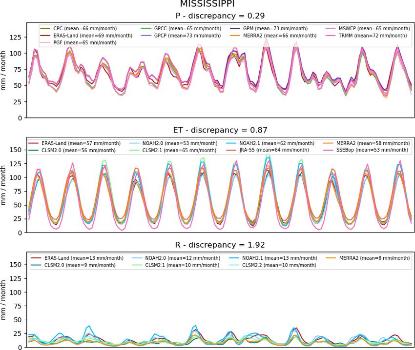
38                                   F. Lehmann et al.: How well are we able to close the water budget at the global scale?

such products varies regionally; thus, satellite-based products    From a group of datasets, the CV is a time series defined
provide a good alternative.                                        as the standard deviation divided by the mean. (A minimum
   Two satellite missions were specifically designed to mea-       value of 10 mm was enforced for the mean to avoid high CVs
sure precipitation. The Tropical Rainfall Measuring Mis-           during the dry season.) The higher the CV, the greater the
sion (TRMM) operated from 1998 to 2015 and provided                disagreement between datasets. Figure S1 in the Supplement
monthly estimations of precipitation over the region from          shows the mean of the CV time series in each basin. Unsur-
50◦ N to 50◦ S. We used the TRMM Multi-satellite Precipi-          prisingly, satellite datasets (TRMM, GPM, and GPCP) pro-
tation Analysis (TMPA) 3B43 version that extends TRMM              vide close results because they use similar measurements and
measurements until 2020 via calibration with other satel-          are, therefore, not at all independent. Observations datasets
lites (Huffman et al., 2007, 2010). The Global Precipita-          (CPC, CRU, and GPCP) are more independent, which leads
tion Measurement (GPM) mission was built on TRMM find-             to higher CVs. However, apart from Australia, where CRU
ings since its launch in February 2014. This constellation         led to precipitation values that were consistently smaller than
of satellites is calibrated using previous satellites through      CPC and GPCC, there were no common patterns in the other
the Integrated Multi-satellitE Retrievals for GPM (IMERG)          regions. In addition, the major differences between reanaly-
to provide global coverage from 2000 onwards (Huffman              ses were found in Central Asia where MERRA2 gave much
et al., 2019). Finally, the Global Precipitation Climatol-         lower precipitation values than ERA5-Land and JRA-55. In-
ogy Project (GPCP) merges various satellite-based estimates        terestingly, Fig. S1 also shows that the method used to cre-
with rain-gauge measurements from the GPCC (Adler et al.,          ate the dataset (i.e. rain-gauge observations, satellite mea-
2018). It provides a well-used and long dataset spanning           surements, or reanalyses) is less relevant than differences
from 1979 to the present.                                          within a method. The inter-category CV measuring differ-
   Apart from these, reanalyses products provide consis-           ences between the mean of observations, satellite, and reanal-
tent estimations of precipitation, evapotranspiration, and         yses datasets was found to be relatively low. The highest CVs
runoff. ERA5-Land is a rerun of the land component from            were found in high-latitude basins where reanalyses consis-
the ERA5 reanalysis developed by the European Centre               tently led to higher precipitation values whereas observations
for Medium-Range Weather Forecasts (ECMWF). Precipi-               had the lowest precipitation values.
tation data are obtained from satellite measurements includ-
ing but not restricted to TRMM and GPM results and are             2.2.2   Evapotranspiration datasets
provided from 1981 onwards (Muñoz-Sabater, 2019). The
Japanese 55-year Reanalysis (JRA-55) also derives precip-          Evapotranspiration is the sum of evaporation from water sur-
itation from satellite measurements with forecasts starting        faces and transpiration through vegetation. Datasets used in
in 1958 (Kobayashi et al., 2015). Finally, the Modern-Era          this study are listed in Table S2. One of the most accu-
Retrospective Analysis for Research and Applications, ver-         rate methods to estimate evapotranspiration is the Penman–
sion 2 (MERRA-2) uses two precipitation datasets from the          Monteith equation (Penman, 1948; Monteith, 1965). The
CPC: the Global Unified Gauge-Based Analysis of Daily              variables used in this equation are obtained from various
Precipitation described above and the Merged Analysis of           land surface parameterisations and energy balance equations
Precipitation which combines gauge-based and satellite mea-        in reanalyses, ERA5-Land and MERRA2, and in GLDAS
surements (Reichle et al., 2017).                                  land surface models (LSMs). We chose three variants of
   Finally, two additional datasets that combine rain-gauge        the GLDAS: the Variable Infiltration Capacity (VIC; Liang
observations, satellite measurements, and reanalyses were          et al., 1994), the Noah model (Chen et al., 1996; Koren
used in this study: the Princeton Global Forcing (PGF)             et al., 1999; Ek et al., 2003), and the Catchment Land
dataset and the Multi-Source Weighted Ensemble Precipi-            Surface Model (CLSM; Koster et al., 2000). These LSMs
tation (MSWEP) dataset. PGF was included as it is one of           are forced with different data depending on the GLDAS
the forcing variables used in the Global Land Data Assim-          version (Rodell et al., 2004). For example, PGF precipita-
ilation System (GLDAS) (Sheffield et al., 2006). Recently          tion was used in version 2.0, GPCP precipitation was used
developed, MSWEP merges gauge observations (including              in version 2.1, and ERA5 precipitation was used in ver-
GPCC), satellite measurements (including TRMM), and re-            sion 2.2 coupled with GRACE data assimilation (for CLSM
analyses (ERA-Interim and JRA-55) (Beck et al., 2019).             only; Li et al., 2019). The MOD16 algorithm also uses
   As there are large disagreements between different              the Penman–Monteith equation with measurements from the
datasets, it is important to assess whether a dataset is in gen-   Moderate Resolution Imaging Spectroradiometer (MODIS,
eral agreement with others. By revealing datasets with sig-        NASA) (Mu et al., 2011).
nificant bias, this method can limit the occurrence of error          One of the main drawbacks of the Penman–Monteith
cancellation, which is a well-known problem in water bud-          equation is the reliance on a large number of parameters,
get studies (Sneeuw et al., 2014; Lorenz et al., 2014). We         such as vegetation characteristics, air temperature, wind, and
have used the coefficient of variation (CV) to evaluate var-       vapour pressure. As these parameters can be difficult to
ious datasets of a water budget component in each basin.           assess accurately, alternative approaches have been devel-

Hydrol. Earth Syst. Sci., 26, 35–54, 2022                                             https://doi.org/10.5194/hess-26-35-2022
F. Lehmann et al.: How well are we able to close the water budget at the global scale?                                         39

oped. For example, the Global Land Evaporation Amsterdam          and runoff measurements and validated against independent
Model (GLEAM) uses an equation involving fewer parame-            river discharge observations from the GRDC.
ters, the Priestley–Taylor equation (Martens et al., 2017; Mi-       As for precipitation and evapotranspiration, Fig. S3 shows
ralles et al., 2011). Another method relies on the energy bud-    the coefficients of variation. CVs were generally higher for
get to compute the fraction of energy leading to water va-        runoff than that for evapotranspiration and precipitation.
porisation, as done in the Simplified Surface Energy Balance      Even though it reflects high uncertainties in runoff values,
for operational applications (SSEBop) (Senay et al., 2013).       this should play a relatively smaller role in the water balance
Finally, algorithms also take advantage of the FLUXNET            because the runoff is the smallest water cycle component.
network of eddy-covariance towers measuring evapotranspi-         In Fig. S3, the inter-category CVs were computed between
ration. To this extent, the machine learning FLUXCOM al-          GRUN, the mean of LSMs, and the mean of reanalyses.
gorithm (Jung et al., 2019) extends the methodology of the        The general observations are complementary to those made
well-used Multi-Tree Ensemble (Jung et al., 2009) by ex-          about evapotranspiration. VIC generally led to the highest
ploiting relationships between meteorological variables and       values among all datasets. Reanalyses tended to be lower,
latent heat flux measured by eddy-covariance towers.              along with CLSM. Finally, compared to the mean across all
   Similar to precipitation, Fig. S2 shows the coefficient        datasets, GRUN was relatively close in general (not shown).
of variation for different categories of evapotranspiration       The largest differences were found in Australia and Central
datasets. CVs were relatively low between the mean of all         Africa, where GRUN was lower, as well as in Central Asia,
categories, as was found for precipitation. The largest differ-   where it led to higher values.
ences between reanalyses were also found in Central Asia,
with MERRA2 predicting lower evapotranspiration. In ad-
dition, it is striking to see the large CVs among land surface    3     Methods
models (CLSM, Noah, and VIC with versions 2.0 and 2.1). In
                                                                  3.1    Water budget reconstruction
this category, there were consistent patterns across all basins
with VIC tending to underestimate ET while CLSM provided          GRACE mascon fields were used to compute time series of
slightly larger values. The CVs were especially large in high-    TWS anomalies relative to the mean between 2004 and 2009.
latitude basins due to low ET in the cold season. Moreover, in    As Eq. (1) involves the variation of TWS over a time period,
Fig. S2, we see that the differences between remote sensing       which is called the terrestrial water storage change (TWSC),
datasets (FLUXCOM, GLEAM, MOD16, and SSEBop) are                  to obtain TWSC from TWS anomalies, the time derivative
not spatially consistent. In Australia, MOD16 led to signif-      was computed with centred finite difference (as in e.g. Long
icantly lower ET, especially during the hot season (October       et al., 2014, or Pascolini-Campbell et al., 2020):
to February). In South Africa, differences were constant all
year long, with MOD16 being lower while FLUXCOM was                               TWS(t + 1) − TWS(t − 1)
rather high. We do not comment on CVs in hot deserts (the         TWSC(t) =                               ,                   (2)
                                                                                           21t
Sahara, the Arabian Peninsula, and Central Asia) because
FLUXCOM and MOD16 are not available in non-vegetated              where 1t equals 1 month, and t − 1, t, and t + 1 are three
land areas.                                                       consecutive months. Missing monthly values were filled with
                                                                  cubic interpolation. In order to match the temporal shift in-
2.2.3   Runoff datasets                                           duced by the central difference, time series of P , ET, and
                                                                  R also needed to be time-filtered by Eq. (3) (Landerer et al.,
Runoff is computed in LSMs as the excess water not evap-          2010):
orated from soils. This water infiltrates through the soil to            1          1      1
the lowest layers without communicating with adjacent grid        X̃(t) = X(t − 1) + X(t) + X(t + 1),                         (3)
                                                                         4          2      4
cells. All of the LSMs presented above provide runoff esti-
mates that were included in this study. River discharge mea-      where X denotes either P , ET, or R. All variables referred
surements are also available from gauge records, but they are     to hereafter are filtered variables but are denoted without the
not temporally consistent across the study period. In addi-       tilde notation for the sake of clarity.
tion, discharge areas from the gauge stations with the longest       Each triplet of datasets (dataP , dataET , dataR ) was called
records do not necessarily match the area of GRDC basins          a combination and led to a budget reconstruction of
that we selected. Therefore, we decided to use only spa-          TWSC computed with Eq. (1): TWSCbudget (t) = PdataP (t) −
tially and temporally consistent datasets by excluding gauge      ETdataET (t) − RdataR (t). This reconstruction was compared
records from our analyses. However, we used the recently          with the derivatives obtained from Eq. (2) and denoted
developed machine learning Global Runoff (GRUN) Recon-            TWSCGRACE (t). As we used 11 precipitation, 14 evapo-
struction dataset which provides runoff values at a 0.5◦ ×0.5◦    transpiration, and 11 runoff datasets, we finally evaluated
spatial resolution from 1902 to 2014 (Ghiggi et al., 2019).       1694 combinations.
This algorithm was trained with precipitation, temperature,

https://doi.org/10.5194/hess-26-35-2022                                               Hydrol. Earth Syst. Sci., 26, 35–54, 2022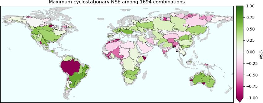
40                                     F. Lehmann et al.: How well are we able to close the water budget at the global scale?

3.2   Metrics

Differences between two time series are commonly evaluated
with the root mean square deviation (RMSD):
          v
               T
          u
          u1 X                                   2
RMSD = t           TWSCbudget (t) − TWSCGRACE (t) . (4)
            T t=1

The main drawback of the RMSD is that it is not normalised
(i.e. basins with large TWSC tend to have larger RMSD).
A very common normalisation is the Nash–Sutcliffe effi-
ciency (NSE) introduced by Nash and Sutcliffe (1970) to
evaluate modelled runoff compared to observations:
                 T                                      2         Figure 2. The cyclostationary NSE is related to the NSE through
             1   P
             T         TWSCbudget (t) − TWSCGRACE (t)                                                  2
                                                                                                      δcst
                 t=1
                                                                   NSEc = 1 − γ + γ NSE, where γ =     2 .
                                                                                                      δcyc
NSE = 1 −
                   T                                  2
             1    P
             T         TWSCGRACE (t) − TWSCGRACE
                 t=1
             RMSD2                                                              1
                                                                                     T
                                                                                     P                                   2
      = 1−     2
                   ,                                         (5)                T          TWSCbudget (t) − TWSCGRACE (t)
              δcst                                                                   t=1
                                                                   NSEc = 1 −
                                                                                       T                                  2
                                                                                 1
                               T                                                           TWSCGRACE (t) − TWSCm
                                                                                      P
                           1   P                                                 T                             GRACE
where TWSCGRACE =          T       TWSCGRACE (t) is the long-                        t=1
                             t=1
term mean of TWSC,         and δcst
                                 is the deviation of monthly                    RMSD2
                                                                         = 1−         ,                                        (6)
values from the long-term mean. In our case, any positive                         2
                                                                                 δcyc
value of the NSE means that the budget reconstruction of
TWSCGRACE is a better approximation than the long-term             where TWSCm     GRACE is the mean value for month m over
mean. The maximum value of 1 describes a perfect recon-            all years, and δcyc is the deviation of GRACE TWSC from
struction, and a negative value denotes poor performance.          the periodic monthly signal. Similarly to the NSE, positive
One major advantage of the NSE is that it requires both phase      values of the cyclostationary NSE indicate a budget recon-
agreement (usually assessed with the correlation coefficient)      struction better than the mean annual cycle, which measures
and a small long-term mean error (evaluated with the bias or       the ability of the reconstruction to capture anomalous events
percentage bias) to yield high values (Lorenz et al., 2014).       (Lorenz et al., 2015; Tourian et al., 2017).
   However, although several attempts have been made to               Moreover, one can express the cyclostationary NSE in
associate positive NSE values to performance (e.g. Henrik-         terms of the NSE by combining Eqs. (5) and (6) as follows:
sen et al., 2003; Samuelsen et al., 2015), it is known that                          2
                                                                                         !
this index suffers from several weaknesses; for example, a                          δcst     δ2
                                                                   NSEc = 1 − 2            + 2cst NSE.                       (7)
high positive NSE can be obtained with a poor time series                           δcyc    δcyc
if the time series has a large variance (Jain and Sudheer,                                  |{z}
                                                                                               γ
2008). In the context of the current study, basins with large
seasonal variations of TWSC, especially tropical basins, are       The γ factor describes the behaviour of the TWSC by com-
more likely to exhibit a NSE close to one even though the          parison with the mean seasonal cycle. Basins with peri-
budget reconstruction presents substantial errors.                 odic seasonal cycles (i.e. low δcyc ) or large magnitudes (i.e.
   To overcome this issue, it has been proposed to com-            high δcst ) have larger γ . In those basins (e.g. the Amazon
pare the budget reconstruction to the mean monthly value           or Chad basins), extremely high NSE values are required to
of TWSC instead of comparing it to the constant long-              achieve a positive cyclostationary NSE, as can be seen in
term mean. The so-called cyclostationary NSE (Thor, 2013;          Fig. 2. Special attention must then be given when examin-
Zhang, 2019) is then expressed as follows:                         ing such basins to discriminate performance depending on
                                                                   the NSE or the cyclostationary NSE.

                                                                   3.3   Selection of the most representative datasets

                                                                   When estimating a water cycle component from the water
                                                                   balance equation (Eq. 1), it is useful to know beforehand

Hydrol. Earth Syst. Sci., 26, 35–54, 2022                                                https://doi.org/10.5194/hess-26-35-2022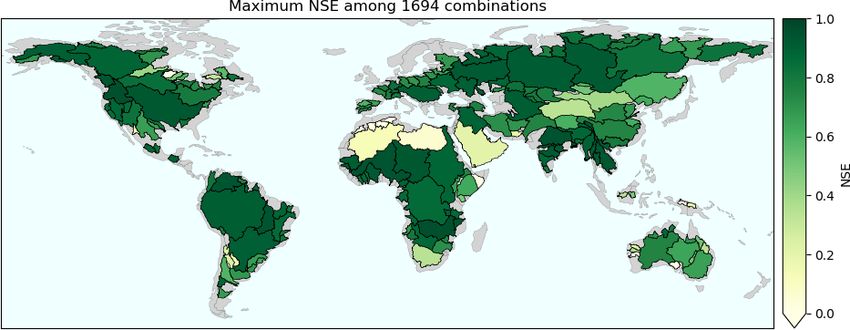
F. Lehmann et al.: How well are we able to close the water budget at the global scale?                                                41
                                                                                       s
which datasets are more reliable to close the water budget                                 1694
                                                                                                 (cib1 − cib2 )2 . For two basins to have
                                                                                            P
                                                                       d(b1 , b2 ) =
in the region under study. This section aims to describe how                               i=1
such datasets can be selected. The NSE results were stored             a small Euclidean distance, each combination i should
in a matrix where each row corresponded to a basin and                 lead to a similar cost in all basins: either the combina-
each column to a combination. Due to the matrix dimension              tion was satisfying in both cases (cib1 ' 0 and cib2 ' 0),
(189×1694), an automated computation was needed to eval-               or it did not perform well in both (cib1 ' 2 and cib2 ' 2).
uate the combinations. This was achieved by introducing a              A hierarchical clustering algorithm was then applied to
cost function which represented the loss of accuracy when              cluster basins so as to minimise the variance between
using any combination instead of the optimal one.                      cost vectors inside a cluster (Mueller et al., 2011).
   Our method can be summarised as follows:
 1. compute the cost matrix to describe the performance of          3. Finally, the maximal cost for combinations to be consid-
    each combination;                                                  ered as satisfying the water budget closure was chosen
                                                                       to be 0.1. This means that the difference between the
 2. cluster basins into larger zones depending on the simi-            RMSD of a suitable combination and the lowest RMSD
    larities between cost vectors;                                     over all combinations is, on average, lower than A/10,
                                                                       where A is the mean seasonal amplitude of TWSC. This
 3. for each zone, select the combinations satisfying a max-
                                                                       threshold guarantees that selected combinations a per-
    imum cost and extract the underlying datasets.
                                                                       formance similar to the optimal combination. Then, in
  In more detail, the following steps were performed:                  each cluster determined by the algorithm, we selected
                                                                       the combinations with a cost lower than 0.1 for all
 1. Using a cost function instead of the absolute metrics              basins in the cluster. From the selected combinations,
    allowed us to overcome the lack of a NSE scale. On                 we extracted the underlying datasets of P , ET, and R.
    the one hand, there are significant differences between            By reporting the number of combinations in which each
    a combination leading to a budget reconstruction with a            dataset appeared, we could evaluate whether a dataset
    NSE close to 0 and another leading to an almost perfect            was clearly better than the others in a given region.
    reconstruction (NSE close to 1). These differences can
    be seen, for example, in terms of months where the bud-
    get reconstruction is within the confidence interval from   4     Results and discussion
    GRACE TWSCs. Therefore, we want to favour combi-
    nations leading to the highest NSE values. On the other     4.1    Water budget closure
    hand, one cannot determine a NSE threshold assuring a
    satisfying reconstruction in all basins. Figure 2 shows     In order to assess the global water budget closure, we first
    that very high NSE values were needed in basins with        examined the instances with the best performance across all
    large γ to outperform the monthly periodic signal. Con-     combinations. This means that, for each basin, we reported
    sequently, a cost function evaluates the performance of     the highest NSE among all 1694 combinations. Figure 3
    a combination relative to the largest NSE achievable in     shows the maximum NSE that can be achieved from a com-
    each basin. The cost function was then defined from the     bination. Please note that a positive NSE was obtained over
    NSE by                                                      99 % of the total study area. Only 9 basins out of 189 did
                                                                not achieve a positive NSE for any combination. These were
    cib = maxcomb NSEb (comb) − NSEb (combinationi ) ,    (8)   mainly hot arid deserts in the northern Sahara, Somalia, and
    where the maximum was computed over all 1694 com-           Australia as well as two other basins in Papua New Guinea
    binations. We emphasise that the cost was evaluated         (Mamberamo Basin) and Canada (Hayes Basin) (Fig. 3). The
    independently for each basin (denoted by the super-         poor performance in arid basins can be explained by limited
    script “b”), allowing the maximum NSE to be different       precipitation and water storage variations that lead to a low
    in each basin. For combinations leading to a cost larger    signal-to-noise ratio. This is a major difference from previ-
    than 2 (i.e. a NSE below −1), the cost was restricted       ous studies where, for example, Lorenz et al. (2014) found
    to 2. This limited the penalisation of combinations with    that only 29 basins out of 96 achieved a positive NSE.
    highly negative values but had no major influence on           Figure 3 can be interpreted as follows: all of the basins
    our results because we focused on the best performing       with a positive NSE offer a budget reconstruction better than
    combinations.                                               the long-term mean from GRACE TWSC. In addition, higher
                                                                NSE values correspond to a better fit between reconstructed
 2. From the cost matrix, each basin could be represented       TWSC and GRACE TWSC. Figure S4 then shows the distri-
    by a vector of 1694 costs. The similarities between         bution of the maximum NSE. Although it has been explained
    two basins b1 and b2 were evaluated based on the Eu-        (in Sect. 3.2) that positive NSE should be interpreted cau-
    clidean distance between their respective cost vector,      tiously, one can observe that 61 % of the study area satis-

https://doi.org/10.5194/hess-26-35-2022                                                Hydrol. Earth Syst. Sci., 26, 35–54, 2022
42 F. Lehmann et al.: How well are we able to close the water budget at the global scale? Figure 3. Maximum NSE per basin over all combinations. Green positive values mean that the budget reconstruction is a better approximation of GRACE TWSC than the long-term mean. fied a NSE larger than 0.8, which is usually considered very ([−100; 100 mm per month]), the NSE was still very high good performance (e.g. Henriksen et al., 2003; Samuelsen (max NSE = 0.91) and could mislead us into concluding that et al., 2015). Given the large number of datasets, it is likely the budget reconstruction is excellent. However, when as- that cancellation of errors explains some of the instances sessing the cyclostationary NSE (max NSEc = −1.28), it ap- with good performance. The reader should remain cautious peared that the mean monthly values were a better fit to about this possibility when trying to reproduce our results GRACE values than the budget reconstruction (Fig. S5). and may use discrepancy measures such as the CV to exam- The underestimation of annual variability in TWSC can be ine datasets, as explained in the following sections. seen in the correlation plot between GRACE TWSC and our By definition, the NSE can only be used to compare the approximation (Fig. S6). Due to the error in approximating budget reconstruction with the long-term mean. As predict- the largest TWSC, the regression slope is 0.7, while 1 is the ing intra-annual variations of TWSC would be more bene- optimal value. Figure S5 additionally shows that the water ficial for hydro-meteorological studies, the cyclostationary balance error is larger than GRACE uncertainty in 21 % of NSE was also used to assess the quality of reconstructed months, meaning that the error is significant. TWSC. Figure 4 shows that a positive maximum cyclosta- However, one should not conclude that all basins with tionary NSE was achieved over 62 % of the study area. It a high NSE and negative cyclostationary NSE exhibit the means that, in those basins, the reconstructed TWSC was same behaviour. The Niger Basin is indeed another basin better than the mean annual cycle obtained from GRACE with a high NSE (0.94) and a negative cyclostationary TWSC. The budget reconstruction performed especially well NSE (−0.62). Contrary to the Amazon, there was no con- in the continental United States (CONUS) and Central Amer- sistent pattern in the water closure error, and the error was ica, in most of South America except the Amazon and the lower than GRACE uncertainty in 94 % of months (Fig. S7). Andes, and in southern Africa, Australia, Europe, western The regression slope was also almost perfect, as shown in Russia, and East Asia (Fig. 4). Fig. S8. In such a basin with low inter-annual variability, the When comparing Figs. 3 and 4, one can observe that de- error between GRACE TWSC and the mean monthly signal spite a very high NSE, some basins could not reach a posi- is very low (RMSD = 6.6 mm per month). Therefore, achiev- tive cyclostationary NSE. This occurrence was especially no- ing a budget reconstruction more accurate than the monthly ticeable in tropical basins like the Amazon and some catch- signal may be an unrealistic expectation. ments in western Africa, India, and Myanmar. These basins In conclusion, while the cyclostationary NSE is useful to illustrate (i) the limits of the NSE and (ii) the need for a assess intra-annual variations in the budget reconstruction, it complementary metric to evaluate the reconstruction. These is not the best assessment tool for all of the tropical basins two points corroborate the conclusions of Jain and Sudheer with almost periodic TWSC. The regression slope between (2008). The Amazon Basin exemplifies why the NSE should the reference and approximate TWSC can help in exhibiting not be used alone to assess the water budget closure. In consistent patterns in the water balance error. fact, even with the best combination, the budget reconstruc- tion consistently underestimated the magnitude of the TWSC 4.2 Variables influencing the water budget closure (Fig. S5). TWSC was too low in the wet season (January– March) and too high in the dry season (July–August). This Several studies have limited their budget computation to indicates that the budget reconstruction was not good enough large catchments only due to the general notion that the ac- to capture the inter-annual and annual variability in TWS. curacy of budget closure increases with the size of the basin. Due to the large amplitude of TWSC in the Amazon Basin We found that both small and large basins can achieve a high Hydrol. Earth Syst. Sci., 26, 35–54, 2022 https://doi.org/10.5194/hess-26-35-2022
F. Lehmann et al.: How well are we able to close the water budget at the global scale?                                            43

Figure 4. Maximum cyclostationary NSE per basin over all combinations. Green positive values mean that the budget reconstruction is a
better approximation of GRACE TWSC than the mean monthly values.

                                                                     imbalance error is rather consistent inside a given climate
                                                                     zone. In the “equatorial rain forest/monsoon” climate zone,
                                                                     basins generally reached higher NSE values (map Fig. 3).
                                                                     However, this zone also contains small Pacific islands (Papua
                                                                     New Guinea and Borneo) where runoff is much higher than
                                                                     evapotranspiration. Tables S3 and S4 indicate that runoff
                                                                     was more uncertain (disagreements of around 30 % between
                                                                     datasets) than evapotranspiration (around 18 %) in those
                                                                     basins. Thus, Pacific islands with large runoff probably suf-
                                                                     fered from poor runoff quality which led to low NSE values.
                                                                        Hot arid deserts also have a large spread in the water bud-
                                                                     get imbalance (Fig. 6). Among those basins, some were en-
                                                                     tirely desert (the Arabian Peninsula, the Sahara, Somalia, and
                                                                     South and West Australia) with a low signal-to-noise ratio,
                                                                     as previously mentioned. Other basins were partially cov-
Figure 5. Each basin is represented by a bar between the maximum     ered by steppe (Australia, the Orange Basin, and around the
NSE (dot) and the 10th highest NSE.                                  Indus Basin) or equatorial savannah (Niger, Chad, and Nile
                                                                     basins). In those basins, precipitation occurred in the more
                                                                     humid subregions, thereby increasing TWS variations. As a
NSE (see Fig. 3). Furthermore, Fig. 5 proves that there is           consequence, the error in the datasets became less significant
indeed no correlation between the maximum NSE and the                and allowed a proper budget reconstruction.
basin area (R 2 = 0.12, p = 0.12). Although limiting their
study to 10 large river basins worldwide, Sahoo et al. (2011)        4.3   Overall combinations’ performance
found no relationship between budget closure error and basin
size. We extend this result and show that basins as small as         Although a majority of basins achieved a positive cyclosta-
65 000km 2 can close the water budget. This result still holds       tionary NSE, they differed greatly in terms of the number
if we evaluate the correlation between the basin area and the        of combinations yielding positive values. As an example,
maximum cyclostationary NSE (R 2 = 0.01, p = 0.90).                  839 combinations satisfied a positive NSEc in the São Fran-
   Figure 5 additionally indicates the consistency of our find-      cisco Basin whereas only 94 did so in the neighbouring To-
ings. Each basin was represented by a bar between the high-          cantins Basin (Fig. S9). Therefore, we wanted to evaluate
est and 10th highest NSE values, and the length of the bar           the ability of a single combination to close the water budget
was smaller than 0.15 in 90 % of the basins. This means              worldwide. To do so, we evaluated the total area of basins
that several combinations were able to close the water budget        with a positive cyclostationary NSE for each combination.
with similar imbalance errors.                                       Table 1 shows the 20 combinations leading to the largest
   Additionally, basins can be classified depending on their         area.
climate zone. Figure 6 shows the distribution of the maxi-              It appears that choosing all three variables (P , ET, and R)
mum NSE in each climate zone. As the boxes (interquartile            from ERA5-Land yields significantly better results than the
range) are of limited length (except for “equatorial rain for-       other combinations (35.5 ×10⁶ km2 with a positive NSEc
est/monsoon” and “hot arid deserts”), this suggests that the         from the total study area of 96.6 ×10⁶ km2 ). Figure 7 in-

https://doi.org/10.5194/hess-26-35-2022                                                Hydrol. Earth Syst. Sci., 26, 35–54, 2022
44 F. Lehmann et al.: How well are we able to close the water budget at the global scale? Figure 6. Box plot of the maximum NSE per climate zone. The green line indicates the median, the box extends from the 1st quartile (Q1 ) to the 3rd quartile (Q3 ), whereas whiskers go from Q1 − 1.5(Q3 − Q1 ) (or the minimum value if higher) to Q3 + 1.5(Q3 − Q1 ) (or the maximum value if lower). Circles denote basins lying outside of the whiskers. The numerals represent the number of basins in each climate zone. dicates that ERA5-Land performed well in the central and ble 1 also shows that each variable has a determining impact eastern United States of America (USA), but it failed to pro- on the water budget closure. Indeed, choosing, for example, vide the positive NSEc of Fig. 4 in the mountainous western CLSM2.2 for runoff instead of ERA5-Land (as shown in the basins (Columbia, Great Basin). Again, in a comparison with left column of Fig. 7) led to poorer results in Alaska, Asia, the best possible results, ERA5-Land performed quite poorly and central Africa, whereas it improved NSE values around in the equatorial region of South America (Amazon Basin the Amazon Basin. and above), in Central Eurasia (around the Ob, Aral Sea, and Concerning GLDAS LSMs, it is clear from Table 1 that Indus basins), and in several basins in Europe. CLSM was a globally better LSM than Noah and VIC. When Knowing that at least one combination exists that gives using all variables from the same LSM, we also noted that a positive cyclostationary NSE in 62.3 ×10⁶ km2 , Table 1 GLDAS 2.0 was globally better than version 2.1 for all LSMs shows that even the best combinations were far from ap- (CLSM, Noah, and VIC). As illustrated in the right column proaching this number. This confirms that it is currently of Fig. 7, major differences are observed in Europe, western clearly impossible to achieve a good water budget closure Russia, and Alaska. This can be explained by disagreement with a single combination (Gao et al., 2010; Lorenz et al., between precipitation from GPCP and PGF. For instance, 2014). CLSM2.1 yielded only low NSE values in most of eastern The second-best combination in terms of area satisfying a Europe, whereas version 2.0 of the same model achieved a positive cyclostationary NSE was the CLSM forced with ver- positive cyclostationary NSE. This last finding reflects the sion 2.0 of GLDAS (in particular PGF precipitation). Table conclusion of studies such as Mueller et al. (2011) and Za- 1 shows that 30.8 ×10⁶ km2 reached a positive NSEc with itchik et al. (2010), who found that forcing variables have a this combination. Similar observations to those for ERA5- considerable influence on land surface models’ outputs. Land can be made generally, with good performance in cen- We also point out that the ranking in Table 1 was not sig- tral and eastern USA, southeastern America, and Australia. nificantly modified by discriminating basins on the area sat- CLSM2.0 was more consistent than ERA5-Land in Europe isfying a NSE larger than 0.5 (usually considered as good but less so in Africa. performance) instead of a positive cyclostationary NSE. This When looking at the following combinations, it appeared ensures the reliability of the method used to highlight the that their performance was more similar, compared with the most consistent combinations. differences observed between the two best combinations. Ta- Hydrol. Earth Syst. Sci., 26, 35–54, 2022 https://doi.org/10.5194/hess-26-35-2022
F. Lehmann et al.: How well are we able to close the water budget at the global scale? 45
Table 1. Combinations with the largest area covered with a positive cyclostationary NSE.
Total Total
area area
with with
NSEc > 0 NSE > 0
(×106 km2 ) (×106 km2 )
P: ERA5-Land; ET: ERA5-Land; R: ERA5-Land 35.5 89.7
P: PGF; ET: CLSM2.0; R: CLSM2.0 30.8 90.2
P : ERA5-Land; ET: ERA5-Land; R: CLSM2.2 24.5 79.7
P : PGF; ET: NOAH2.0; R: CLSM2.0 23.9 90.9
P: GPCP; ET: CLSM2.1; R: CLSM2.1 23.4 79.2
P : ERA5-Land; ET: ERA5-Land; R: GRUN 22.7 81.3
P : MSWEP; ET: CLSM2.0; R: CLSM2.0 21.8 78.5
P : ERA5-Land; ET: ERA5-Land; R: CLSM2.0 21.7 78.6
P : ERA5-Land; ET: ERA5-Land; R: MERRA2 21.7 76.6
P : GPM; ET: CLSM2.1; R: CLSM2.1 21.1 80.1
P : GPCP; ET: CLSM2.1; R: CLSM2.0 20.8 78.4
P : GPCC; ET: CLSM2.0; R: CLSM2.0 20.4 79.4
P : ERA5-Land; ET: ERA5-Land; R: NOAH2.0 19.8 84.4
P : GPM; ET: CLSM2.1; R: CLSM2.0 19.0 79.4
P: MERRA2; ET: MERRA2; R: MERRA2 18.8 92.1
P : GPM; ET: NOAH2.1; R: NOAH2.0 18.8 81.0
P : GPM; ET: CLSM2.1; R: CLSM2.2 18.7 71.2
P : GPCP; ET: CLSM2.1; R: CLSM2.2 18.5 74.6
P : TRMM; ET: CLSM2.1; R: CLSM2.1 18.5 56.7
P : PGF; ET: NOAH2.0; R: CLSM2.2 18.4 86.3
... ... ...
P: PGF; ET: VIC2.0; R: VIC2.0 16.1 87.6
... ... ...
P: PGF; ET: NOAH2.0; R: NOAH2.0 16.0 92.4
... ... ...
P: GPCP; ET: NOAH2.1; R: NOAH2.1 13.3 82.6
... ... ...
P: ERA5-Land; ET: CLSM2.2; R: CLSM2.2 10.8 57.8
... ... ...
P: JRA-55; ET: JRA-55; R: JRA-55 8.7 72.2
... ... ...
P: GPCP; ET: VIC2.1; R: VIC2.1 7.1 75.6
Combinations are ranked by decreasing area of basins with a positive cyclostationary NSE. Italics indicate
combinations where P , ET, and R are from the same model.
4.4 Datasets suitable in given regions excellent budget closure could be achieved (maximum NSE
larger than 0.8 or maximum NSEc larger than 0.1).
In general, many combinations were below the maximum
cost: at least 112 combinations were suitable in 50 % of the
In the previous section, numerous combinations of global basins, and at least 185 combinations were suitable in 25 %
datasets were evaluated. This section aims to describe re- of the basins. For a detailed review of suitable datasets in
gions where some datasets are more suitable than others to each basin, the reader is referred to Figs. S17–S20. Although
close the water budget. In a given basin, we defined suit- there was a large choice of combinations to close the water
able datasets as those appearing in combinations leading to a budget, two basins with similar characteristics only had a few
cost (difference between the maximum NSE and the NSE for suitable combinations in common. This makes a global and
a specific combination) lower than 0.1. This threshold was comprehensive evaluation of datasets more complex.
chosen to ensure that only the combinations with the best In addition, we observed that suitable datasets in a basin
performance were considered as suitable. For this analysis, could generally not be mixed, suggesting that some cancella-
we focus on a subset of 132 basins, out of the 189, where an
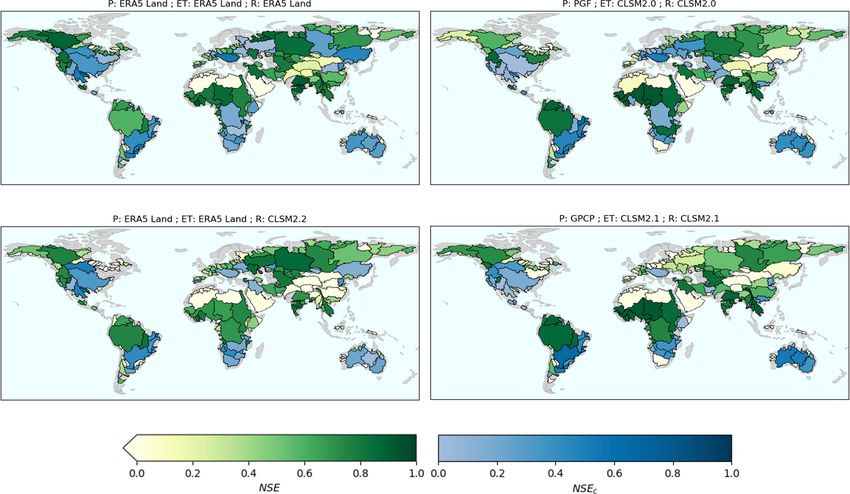
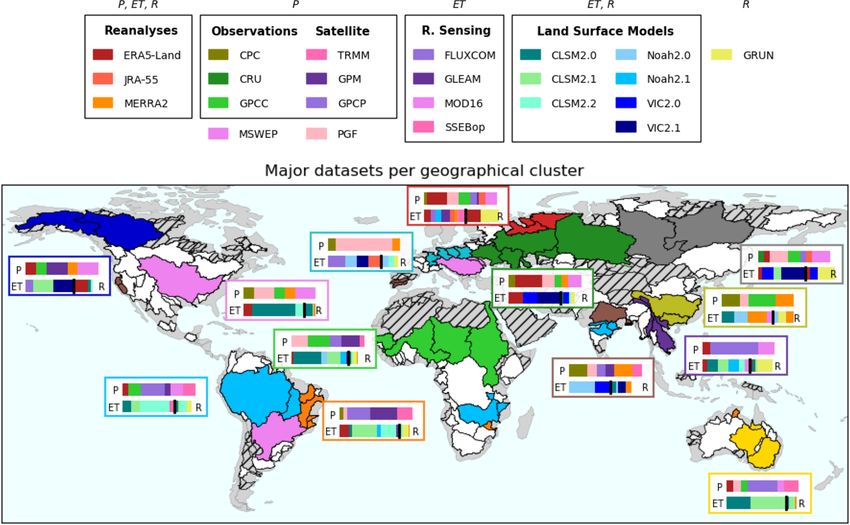
https://doi.org/10.5194/hess-26-35-2022 Hydrol. Earth Syst. Sci., 26, 35–54, 202246 F. Lehmann et al.: How well are we able to close the water budget at the global scale? Figure 7. NSE and cyclostationary NSE with the first combinations in Table 1. Basins with a positive cyclostationary NSE are represented with blue shades corresponding to the NSEc . The remaining basins are depicted in green, according to their NSE. tion bias occurred. As an example, Fig. 8 shows that suitable formed well in those basins. Among basins with similar char- datasets in the Mississippi Basin have considerably different acteristics, we pointed out large rivers in temperate regions seasonal cycles. Combining a precipitation dataset with high (Mississippi, Paraná, and Danube basins) or cold basins with amplitude (GPCP) with low runoff (CLSM2.2) could close different snow conditions (Yenisei, Lena, Mackenzie, Yukon, the water budget if associated with high evapotranspiration and Kolyma basins). (CLSM2.1, leading to NSEc = 0.32) but not with low evap- For each of the 13 clusters, we selected combinations otranspiration (Noah2.0, NSEc = −1.8). As there is no rea- yielding a cost lower than 0.1 in every basin of the region. son to consider one dataset more reliable than others in the Figure 9 shows which datasets can be used in combina- absence of unbiased observations, care must be taken when tion to satisfy the water balance. Among the precipitation combining suitable datasets. datasets, it first appears that the rain-gauge-based GPCC was In order to provide a general overview of datasets’ per- often found in combinations satisfying the maximum cost, formance, we choose to gather basins achieving the wa- along with the satellite-augmented GPCP, reanalysis ERA5- ter budget closure for similar combinations. Those regions Land, and the multi-source PGF. As a first approximation, were determined with the hierarchical clustering described in those datasets are suitable for global water budget analyses. Sect. 3.3. The 132 selected basins with a good water budget However, for regional analyses, a closer look at individual closure are depicted in the dendrogram in Fig. S10, and clus- datasets is required to obtain all possibilities. ters represent basins with similar costs for the same combi- Figure 10 (top left) shows the decay in NSE when using nations. We chose 13 such clusters comprising major basins GPCC as the precipitation dataset. It confirms that GPCC of the world to provide a precise (but succinct as possible) was very close to the best-performing precipitation datasets. overview of the datasets’ performance. These clusters are de- Surprisingly, Fig. 10 also indicates that although GPCP noted by the coloured lines in Fig. S10 and are shown with added satellite measurements to GPCC observations, it in- the same basin colours as on the map in Fig. 9. creased the water budget imbalance in eastern Europe and Basins clustered together in the dendrogram in Fig. S10 western Russia as well as in Congo and South Africa. GPCP were either neighbouring basins (e.g. eastern Europe or east- performed notably well in South America, along with ERA5- ern Australia) or basins with similar geographical conditions. Land, which was one of the most consistent datasets for pre- Therefore, it is sensible that the same combinations per- cipitation. The only region where ERA5-Land was not suit- Hydrol. Earth Syst. Sci., 26, 35–54, 2022 https://doi.org/10.5194/hess-26-35-2022
F. Lehmann et al.: How well are we able to close the water budget at the global scale?                                              47

Figure 8. Datasets appearing in suitable combinations in the Mississippi Basin (cost lower than 0.1). The discrepancy is similar to the
coefficient of variation, except that the numerator is the difference between the maximum and minimum values instead of the standard
deviation.

able was around China and Saint Lawrence Basin. As shown                 Figure 9 clearly shows that evapotranspiration from the
in Fig. 9, PGF precipitation was able to close the water bud-         land surface model VIC should be chosen in Russian snow-
get predominantly in Europe as well as in Central Africa.             dominated basins, with a preference for version 2.0 com-
   For comparison, Fig. S12 indicates that CRU, which never           pared with 2.1. However, this dataset should not be used in
appears in the map Fig. 9, performed very poorly compared             hotter regions such as South America, Africa, or Australia
with other datasets. Harris et al. (2020) mentioned that no ho-       (Fig. S11). We found that VIC produces less evapotranspi-
mogenisation of data was performed in CRU data. CRU also              ration than other datasets, along with higher runoff. CLSM
uses climatology values when measurements are missing,                was also consistently found in Fig. 9. Versions 2.0 and 2.1
making it more appropriate for global analyses. The other             performed similarly (except in Europe, where version 2.0
rain-gauge-based dataset CPC was mainly suitable in Europe            was better, as already mentioned) and were especially suit-
and China (see Fig. 9). As MERRA2 is based on CPC obser-              able in equatorial (South America, sub-Saharan Africa, and
vations (except in Africa, where slight variations can be seen        Australia) and some temperate regions (southeastern Europe
in Fig. S12), similar conclusions can be drawn for MERRA2.            and the USA). Similar to precipitation, ERA5-Land evapo-
In addition, using GPM instead of TRMM (where we recall               transpiration is an excellent dataset in most of the regions
that GPM includes and extends TRMM results) improved the              except the Amazon Basin, China, and Australia (Fig. S11).
water budget closure. Finally, there was no overwhelming                 Evapotranspiration from CLSM version 2.2 provided a
advantage in choosing the multi-source MSWEP dataset; it              good water budget closure in most of South America, Eu-
is consistent in Europe and South America but should be               rope, and especially South Asia. However, it led to unrealis-
avoided in snow-dominated regions of eastern Russia and               tic low values in snow-dominated basins (see Fig. S11). An
Alaska (Fig. S12).                                                    example of this behaviour is given in Fig. S15 where highly
                                                                      negative values appear in autumn. As this dataset assimilates

https://doi.org/10.5194/hess-26-35-2022                                                  Hydrol. Earth Syst. Sci., 26, 35–54, 2022
48 F. Lehmann et al.: How well are we able to close the water budget at the global scale? Figure 9. Datasets appearing in combinations that satisfy a cost lower than 0.1 for all basins inside the cluster. The 13 clusters highlighted in Fig. S10 are shown using different colours. For each cluster, the top line of each box represents precipitation datasets. The left part of the bottom line is evapotranspiration datasets whereas the right part is runoff. The limit between ET and R is symbolised by a black line located proportionally to the portion of ET in the mean annual water cycle of the corresponding region. Hatched areas show basins with a poor water budget closure (maximum NSE lower than 0.8 and maximum NSEc lower than 0.1). Figure 10. The mean of the 10th highest NSE with combinations comprising the reference dataset (i.e. GPCC, GPCP, PGF, or ERA5-Land) is compared to the mean of the 10th highest NSE excluding the reference dataset. Yellow indicates basins where the reference dataset is similar to or better than other precipitation datasets whereas blues show regions where it was significantly worse. Hatched areas show basins with a poor water budget closure (maximum NSE lower than 0.8 and maximum NSEc lower than 0.1). Hydrol. Earth Syst. Sci., 26, 35–54, 2022 https://doi.org/10.5194/hess-26-35-2022
You can also read