Exploration of the atmospheric chemistry of nitrous acid in a coastal city of southeastern China: results from measurements across four seasons
←
→
Page content transcription
If your browser does not render page correctly, please read the page content below
Research article
Atmos. Chem. Phys., 22, 371–393, 2022
https://doi.org/10.5194/acp-22-371-2022
© Author(s) 2022. This work is distributed under
the Creative Commons Attribution 4.0 License.

       Exploration of the atmospheric chemistry of nitrous acid
         in a coastal city of southeastern China: results from
                 measurements across four seasons
           Baoye Hu1,2,3,4, , Jun Duan5, , Youwei Hong1,2 , Lingling Xu1,2 , Mengren Li1,2 , Yahui Bian1,2 ,
                            Min Qin5 , Wu Fang5 , Pinhua Xie1,5,6,7 , and Jinsheng Chen1,2
              1 Center  for Excellence in Regional Atmospheric Environment, Institute of Urban Environment,
                                     Chinese Academy of Sciences, Xiamen 361021, China
                         2 Key Lab of Urban Environment and Health, Institute of Urban Environment,

                                     Chinese Academy of Sciences, Xiamen 361021, China
                            3 Fujian Provincial Key Laboratory of Pollution Monitoring and Control,

                                     Minnan Normal University, Zhangzhou, 363000, China
               4 Fujian Provincial Key Laboratory of Modern Analytical Science and Separation Technology,

                                     Minnan Normal University, Zhangzhou, 363000, China
          5 Key Laboratory of Environment Optics and Technology, Anhui Institute of Optics and Fine Mechanics,

                                      Chinese Academy of Sciences, Hefei, 230031, China
                            6 University of the Chinese Academy of Sciences, Beijing 100086, China
                               7 School of Environmental Science and Optoelectronic Technology,

                              University of Science and Technology of China, Hefei, 230026, China
                                          These authors contributed equally to this work.

                 Correspondence: Jinsheng Chen (jschen@iue.ac.cn) and Min Qin (mqin@aiofm.ac.cn)

                                Received: 25 August 2021 – Discussion started: 23 September 2021
                     Revised: 6 November 2021 – Accepted: 30 November 2021 – Published: 11 January 2022

      Abstract. Because nitrous acid (HONO) photolysis is a key source of hydroxyl (OH) radicals, identifying the
      atmospheric sources of HONO is essential to enhance the understanding of atmospheric chemistry processes and
      improve the accuracy of simulation models. We performed seasonal field observations of HONO in a coastal city
      of southeastern China, along with measurements of trace gases, aerosol compositions, photolysis rate constants
      (J ), and meteorological parameters. The results showed that the average observed concentration of HONO was
      0.54 ± 0.47 ppb. Vehicle exhaust emissions contributed an average of 1.45 % to HONO, higher than the values
      found in most other studies, suggesting an influence from diesel vehicle emissions. The mean conversion fre-
      quency of NO2 to HONO in the nighttime was the highest in summer due to water droplets evaporating under
      high-temperature conditions. Based on a budget analysis, the rate of emission from unknown sources (Runknown )
      was highest around midday, with values of 4.51 ppb h−1 in summer, 3.51 ppb h−1 in spring, 3.28 ppb h−1 in au-
      tumn, and 2.08 ppb h−1 in winter. Unknown sources made up the largest proportion of all sources in summer
      (81.25 %), autumn (73.99 %), spring (70.87 %), and winter (59.28 %). The photolysis of particulate nitrate was
      probably a source in spring and summer while the conversion from NO2 to HONO on BC enhanced by light
      was perhaps a source in autumn and winter. The variation of HONO at night can be exactly simulated based on
      the HONO / NOx ratio, while the J (NO−               −
                                              3 _R) × pNO3 should be considered for daytime simulations in summer
                                   −             −
      and autumn, or 1/4× (J (NO3 _R) × pNO3 ) in spring and winter. Compared with O3 photolysis, HONO pho-
      tolysis has long been an important source of OH except for summer afternoons. Observation of HONO across
      four seasons with various auxiliary parameters improves the comprehension of HONO chemistry in southeastern
      coastal China.

Published by Copernicus Publications on behalf of the European Geosciences Union.
372                                                     B. Hu et al.: Exploration of the atmospheric chemistry of nitrous acid

1   Introduction                                                  ficients of NO2 conversion to HONO on surfaces (including
                                                                  aerosols, ground, buildings, and vegetation) vary from 10−9
                                                                  to 10−2 , derived from different experiments (Ammann et al.,
Nitrous acid (HONO) photolysis produces hydroxyl radical          1998; Kirchner et al., 2000; Underwood et al., 2001; Aubin
(OH), an important oxidant, in the troposphere (Zhou et al.,      and Abbatt, 2007; Zhou et al., 2015; Liu et al., 2014; Van-
2011). OH plays an important role in triggering the oxida-        denboer et al., 2013). It is still a challenge to extrapolate lab-
tion of volatile organic compounds and therefore determines       oratory results to real surfaces. There is still research being
the fate of many anthropogenic atmospheric pollutants (Lei        carried out to distinguish the key step to determine the NO2
et al., 2018). Recent research results have shown that HONO       uptake, and we are also not sure what role radiation plays in
production is the cause of an increase in secondary pollutants    it. The absence of major HONO sources during the daytime
(Li et al., 2010; Gil et al., 2019; Fu et al., 2019). Though      is another subject of active ongoing research.
extensive studies have been conducted in the four decades             According to an analysis of 15 sets of field observations
since the first clear measurement of HONO (Perner and Platt,      around the world (Elshorbany et al., 2012), the HONO / NOx
1979), the HONO formation mechanisms are still elusive, es-       ratio (0.02) predicts well HONO concentrations under dif-
pecially during the daytime, when there is a large difference     ferent atmospheric conditions. To avoid underestimation of
between measured concentrations and those calculated from         HONO in this study, an empirical parameterization was ap-
known gas-phase chemistry (Sörgel et al., 2011). Identifica-      plied to estimate the HONO concentration, because the cur-
tion of the sources of atmospheric HONO and exploration           rent understanding of HONO formation mechanisms is in-
of its formation mechanisms are beneficial for enhancing our      complete. Field measurements of HONO and its precursor
comprehension of atmospheric chemistry processes and im-          NO2 at sites with different aerosol load and composition,
proving the accuracy of atmospheric simulation models.            photolysis rate constants, and meteorological parameters are
   Commonly accepted HONO sources include direct emis-            necessary to deepen our knowledge of the HONO forma-
sion from motor vehicles (Chang et al., 2016; Kirchstetter et     tion mechanisms. Such measurements have been carried out
al., 1996; Kramer et al., 2020; Xu et al., 2015) or soil (Su et   in coastal cities in China, including Guangzhou (Qin et al.,
al., 2011; Tang et al., 2019; Oswald et al., 2013), the homoge-   2009), Hong Kong (Xu et al., 2015), and Shanghai (Cui et
neous conversion of NO by OH (Seinfeld and Pandis, 1998;          al., 2018), where the air pollution was relatively severe dur-
Kleffmann, 2007), and the heterogeneous reaction of NO2 on        ing the research period. However, there has been a lack of
humid surfaces (Alicke, 2002; Finlayson-Pitts et al., 2003).      research into HONO in coastal cities with good air quality
Other homogeneous sources include nucleation reactions of         and low concentrations of PM2.5 , but strong sunlight and
NH3 , NO2 , and H2 O (Zhang and Tao, 2010); electronically        high humidity. Insufficient research on coastal cities with
excited H2 O and NO2 for the production of HONO (Li et al.,       good air quality has resulted in certain obstacles to assessing
2008); and the HO2 · H2 O complex and NO2 for the produc-         the photochemical processes in these areas. Due to different
tion of HONO (Li et al., 2014). Other heterogeneous sources       emission-source intensities and ground surfaces, the atmo-
include NO2 reduced on soot to produce HONO and drasti-           spheric chemistry of HONO in the southeastern coastal area
cally enhanced by light (Ammann et al., 1998; Monge et al.,       of China is predicted to have different pollution character-
2010), semivolatile organics from diesel exhaust for the pro-     istics from those found in other coastal cities. Furthermore,
duction of HONO (Gutzwiller et al., 2002), photoactivation        HONO contributes to the atmospheric photochemistry dif-
of NO2 on humic acid (Stemmler et al., 2006), TiO2 (Ndour         ferently depending on the season (Li et al., 2010). Therefore,
et al., 2008), solid organic compounds (George et al., 2005),     observations of atmospheric HONO across different seasons
the photolysis of particulate nitrate by ultraviolet (UV) light   in the southeastern coastal area of China are urgently needed.
(Kasibhatla et al., 2018; Romer et al., 2018; Ye et al., 2017;        Incoherent broadband cavity-enhanced absorption spec-
Scharko et al., 2014), dissolution of NO2 catalyzed by an-        troscopy (IBBCEAS) was employed in this study to deter-
ions on aqueous microdroplets (Yabushita et al., 2009), the       mine HONO concentrations in the southeastern coastal city
process of acid displacement (Vandenboer et al., 2014), the       of Xiamen in August (summer), October (autumn), and De-
conversion of NO2 to HONO on the ground (Wong et al.,             cember (winter) 2018 and March (spring) 2019. In addition,
2011), NH3 enhancing the heterogeneous reaction of NO2            a series of other relevant trace gases, meteorological param-
with SO2 for the production of HONO (Ge et al., 2019),            eters, and photolysis rate constants were measured at the
NH3 promoting NO2 dimer hydrolysis for HONO produc-               same time to provide additional information to reveal the
tion through stabilizing the state of the product and reduc-      HONO formation mechanisms. The main purposes of this
ing the reaction free energy barrier (L. Li et al., 2018; Xu et   study were to (1) calculate the values of unknown HONO
al., 2019), and heterogeneous formation of HONO catalyzed         daytime sources, (2) analyze the processes leading to HONO
by CO2 (Xia et al., 2021). Heterogeneous processes are the        formation, (3) simulate HONO concentrations based on an
most poorly understood and yet are widely considered the          empirical parameterization, and (4) evaluate OH production
main sources of HONO in previous studies. The uptake coef-

Atmos. Chem. Phys., 22, 371–393, 2022                                                https://doi.org/10.5194/acp-22-371-2022
B. Hu et al.: Exploration of the atmospheric chemistry of nitrous acid                                                     373

from HONO from 07:00 to 16:00 local time (LT). These re-         proximately 25 ± 0.01 ◦ C by using a thermoelectric cooler
sults were compared between the seasons.                         unit. In order to prevent particulate matter from entering
                                                                 the cavity and reducing the effect of particulate matter on
                                                                 the effective absorption path, a 1 µm polytetrafluoroethylene
2     Methodology
                                                                 (PTFE) filter membrane (Tisch Scientific) was used in the
2.1    Site description
                                                                 front end of the sampling port. In order to ensure the quality
                                                                 of the data, the 1 µm PTFE filter membrane was usually re-
Our field observations were carried out ∼ 80 m above the         placed once every three days and the sampling tube was thor-
ground at a supersite located on the top of the Administra-      oughly cleaned with alcohol once a month. We increased the
tive Building of the Institute of Urban Environment (IUE),       replacement frequency of the filter membrane and the clean-
Chinese Academy of Sciences (118◦ 040 1300 E, 24◦ 360 5200 N),   ing frequency of the sampling tube in the event of heavy pol-
in Xiamen, China, in August, October, and December 2018          lution to ensure that the filter membrane and sampling tube
and March 2019 (Fig. 1). The supersite was equipped with         are in a clean state. The length of sampling tube with 6 mm
a complete set of measurement tools, including those for         outer diameter was approximately 3 m, the material was PFA
measuring gases and aerosol species composition, meteorol-       with excellent chemical inertness, and the sampling flow rate
ogy parameters, and photolysis rate constants, which pro-        was 6 SLM meaning that the residence time of the gas in
vided a good chance to study the atmospheric chemistry of        the sampling tube was less than 0.5 s. Besides, the sampling
HONO in a coastal city of southeastern China. As shown in        loss was calibrated before the experiment. We assessed the
Fig. 1 (left), Xiamen is located at the southeastern coastal     measured spectrum every day to ensure the authenticity of
area of China and faces the Taiwan Strait in the east. It suf-   the measurement results. Multiple reflections in the resonator
fers from sea and land breeze throughout the year with spring    cavity enhanced the length of the effective absorption path,
and summer more frequently (Xun et al., 2017). The IUE           thereby enhancing the detection sensitivity of the instrument.
supersite is surrounded by Xinglin Bay, several universities     The 1σ detection limits for HONO and NO2 were about 60
(or institutes), and several major roads with a large traffic    and 100 ppt, respectively, and the time resolution was 1 min.
fleet, such as Jimei Road, Shenhai Expressway (870 m), and       The fitting wavelength range was selected as 359–387 nm.
Xiasha Expressway (2300 m) (Fig. 1 (right)). The area of         The measurement error of HONO of IBBCEAS was esti-
Xiamen is 1700.61 km2 with a population of 4.11 million          mated to be about 9 %, considering both HONO secondary
(http://tjj.xm.gov.cn/tjzl/, last access: 12 August 2019). The   formation and sample loss. The sampling tube was heated
number of motor vehicles in 2018 was 1 572 088, which was        to 35 ◦ C and covered by insulation cotton materials to pre-
2.73 times as many as 10 years ago. The surrounding soil is      vent the effect of condensation of the water vapor (Lee et al.,
used for landscape greening, not for agricultural production.    2013).
                                                                    The inorganic composition of PM2.5 aerosols (SO2−       4 ,
2.2    Instrumentation
                                                                 NO− 3 , Cl − , Na+ , NH+ , K+ , Ca2+ , and Mg2+ ) and concen-
                                                                                        4
                                                                 trations of gases (HONO, HNO3 , HCl, SO2 , NH3 ) were de-
The atmospheric concentrations of both HONO and NO2              termined using a Monitor for AeRosols and Gases in am-
were determined using IBBCEAS, which has previously              bient Air (MARGA, Model ADI 2080, Applikon Analyt-
been widely applied to such measurements (Tang et al., 2019;     ical B.V., the Netherlands). Ambient air was drawn into
Duan et al., 2018; Min et al., 2016). The IBBCEAS instru-        the sample box by a PM2.5 cyclone (Teflon coated, URG-
ment was customized by the Anhui Institute of Optics and         2000-30ENB) at the flow rate of 1 m3 h−1 . Air sample was
Fine Mechanics (AIOFM), Chinese Academy of Sciences              drawn firstly through the wet rotating denuder (WRD) where
(Duan et al., 2018). The resonant cavity is composed of a pair   gases diffused to the solution, and then particles were col-
of highly reflective mirrors separated by 70 cm, and their re-   lected by a steam jet aerosol collector (SJAC). Absorption
flectivity is approximately 0.99983 at 368.2 nm. The surface     solutions were drawn from the SJAC and the WRD to sy-
of the mirrors was purged by dry nitrogen at 0.1 standard        ringes (25 mL). Samples were injected into Metrohm cation
liters per minute (SLM), and the air flow was controlled by      (500 µL loop) and anion (250 µL loop) chromatographs with
a mass flow controller to prevent the surface of the mirror      the internal standard (LiBr) for 15 min after an hour when
from being contaminated. Light was introduced into the res-      the syringes had been filled (Makkonen et al., 2012). Spe-
onant cavity and was emitted by a single light-emitting diode    cific descriptions of the SJAC can be found in previous re-
(LED) with full width at half maximum (FWHM) of 13 nm            ports (Slanina et al., 2001; Wyers et al., 1993). Therefore,
and a peak wavelength of 365 nm. Light transmitted through       the times needed for the sampling period and the latter IC
the cavity was received by a spectrometer (QE65000, Ocean        analysis on the MARGA system are a full hour and 15 min,
Optics Inc., USA) through an optical fiber with 600 µm di-       respectively. The value measured in this hour is actually the
ameter and a 0.22 numerical aperture.                            concentration sampled in the previous hour, so the time cor-
   In order to avoid the drift of the center wavelength of the   responding to the sampling is matched with other instrument
LED, the temperature of the LED was controlled to be ap-         parameters (i.e., HONO, NOx , J values).

https://doi.org/10.5194/acp-22-371-2022                                            Atmos. Chem. Phys., 22, 371–393, 2022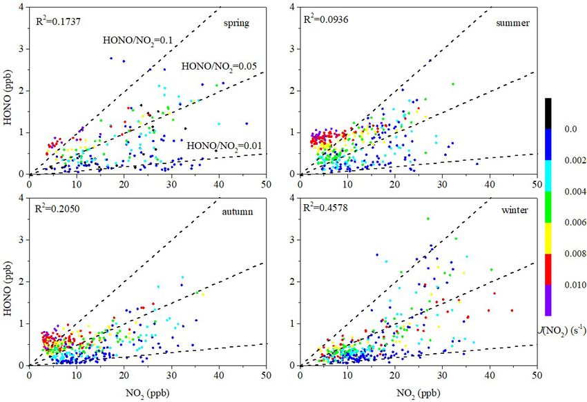
374                                                         B. Hu et al.: Exploration of the atmospheric chemistry of nitrous acid

Figure 1. Location of Xiamen in China (left) and surroundings of IUE (right). Note: the map on the left was directly downloaded from
http://bzdt.ch.mnr.gov.cn/ (last access: 22 September 2021), while the map in the right was significantly enriched based on a layer download
from http://www.rivermap.cn/ (last access: 25 October 2020). The copyright statement of Fig. 1 on the left is © 2021 SinoMaps Press and
National Geomatics Center of China.

   Photolysis frequencies were determined using a photolysis            (Supplement Fig. S1). Therefore, the NO2 concentration as
spectrometer (PFS-100, Focused Photonics Inc., Hangzhou,                measured by IBBCEAS was used in this study. An oscillat-
China). These were calculated by multiplying the actinic flux           ing microbalance with a tapered element was applied to de-
F , quantum yield ϕ(λ) and the known absorption cross sec-              termine the PM2.5 concentration with uncertainty of 10 %–
tion σ (ϕ). The measurements included the photolysis rate               20 %. Black carbon (BC) was measured using an Aethalome-
constants J (O1 D), J (HCHO_M), J (HCHO_R), J (NO2 ),                   ter at 7 wavelengths (in using 880 nm wavelength). When the
J (H2 O2 ), J (HONO), J (NO3 _M), and J (NO3 _R), and                   tape was < 10 %, aethalometer fiber tape was replaced. Me-
the spectral band ranged from 270 to 790 nm. Hemispheri-                teorological parameters were determined by an ultrasonic at-
cal (2π sr) angular response deviations were within ±5 %.               mospherium (150WX, Airmar, USA). The time resolution of
The photolysis rate constants with _R and _M represented                all instruments was unified to 1 h to facilitate comparison. Ul-
a radical photolysis channel and molecular photolysis chan-             traviolet radiation (UV) was determined by a UV radiometer
nel, respectively. Specifically, HCHO was removed by the                (Kipp & Zonen, SUV5 Smart UV Radiometer).
Reactions (R1) and (R2), and NO3 was removed by the Re-
actions (R3) and (R4), respectively (Röckmann et al., 2010).
                                                                        3     Results and discussion
HCHO + hv −→ CHO + H             J (HCHO_R)                   (R1)
HCHO + hv −→ H2 + CO J (HCHO_M)                               (R2)      3.1    Overview of data

NO3 + hv −→ NO2 + O3 P           J (NO3 _R)                   (R3)      Fig. 2 showed an overview of the determined HONO, NO,
NO3 + hv −→ NO + O2           J (NO3 _M)                      (R4)      NO2 , PM2.5 , NO−  3 , BC, J (HONO), temperature (T ), and
                                                                        relative humidity (RH) in this study. The entire campaign
The O3 concentration was determined by an ultraviolet pho-              was characterized by a subtropical monsoon climate with
tometric analyzer (model 49i, Thermo Environmental Instru-              high temperatures (9.82–34.42 ◦ C) and high humidity
ments (TEI) Inc.), and the limit of the instrument is 1.0 ppb.          (29.24 %–100 %). The mean values (± standard deviation)
The NO concentration was determined by a chemilumines-                  of temperature and relative humidity were 22.24 ± 5.41 ◦ C
cence analyzer (TEI model 42i) with a molybdenum con-                   and 78.35 ± 14.07 %, respectively. Elevated concentrations
verter. The detection limit and the uncertainty of the TEI              of NOx , i.e., up to 156.17 ppb of NO and 172.42 ppb of
model 42i were 0.5 ppb and 10 %, respectively. Although                 NO2 , were observed, possibly due to dense vehicle emis-
the TEI model 42i also measures the concentration of NO2 ,              sions near this site. The photolysis rate constants J (O1 D),
this value might actually include other active nitrogen com-            J (HCHO_M), J (HCHO_R), J (NO2 ), J (H2 O2 ), J (HONO),
ponents (Villena et al., 2012). As expected, the NO2 con-               J (NO3 _M), and J (NO3 _R) had the same temporal vari-
centration measured by IBBCEAS had the same trend as                    ation (Fig. S2), although their orders of magnitude were
the NO2 measured by TEI 42i, and NO2 concentration mea-                 different. The correlation coefficients between J (HONO)
sured by IBBCEAS was always lower than that by TEI 42i                  and other photolysis rate constants were above 0.965 (not

Atmos. Chem. Phys., 22, 371–393, 2022                                                       https://doi.org/10.5194/acp-22-371-2022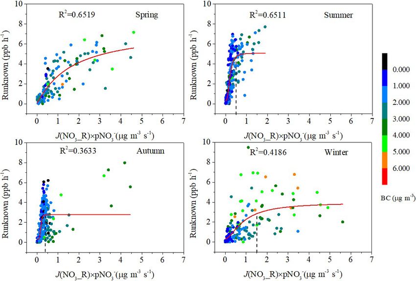
B. Hu et al.: Exploration of the atmospheric chemistry of nitrous acid                                                        375

shown). Both J (HONO) and UV peaked around noon,                   results were found in Hong Kong, which is also a coastal city
and the maximum of J (HONO) (2.02 × 10⁻³ s−1 ) and UV              (Xu et al., 2015). However, most previous studies have found
(55.62 W m−2 ) appeared at 13:00 LT on 11 March 2019, and          that the HONO concentration at night is significantly higher
12:00 LT on 14 August 2018, respectively. This area was            than that during the day (Wang et al., 2015; Liu et al., 2019a;
dominated by photochemical pollution, while particulate            D. Li et al., 2018; Elshorbany et al., 2009; Acker et al., 2006;
pollution was relatively light. No haze episodes occurred          Yu et al., 2009). The higher HONO in the daytime is likely
across four seasons with 111 d, because daily mass con-            due to the higher NOx or nitrate photolysis as discussed in
centration of PM2.5 was lower than the National Ambient            following section.
Air Quality Standard (Class II: 75 µg m−3 ). For O3 , 10              The ratio of HONO to NOx or the ratio of HONO to NO2
episodes occurred with 8 h maximum concentrations of               have been extensively applied to indicate heterogeneous con-
O3 exceeding the Class II: 160 µg m−3 . Maximum mixing             version of NO2 to HONO (Li et al., 2012; Liu et al., 2019a;
ratio of O3 was 113.81 ppb, occurring in the afternoon with        Zheng et al., 2020). Compared with the HONO / NO2 ra-
strong ultraviolet radiation (42.72 W m−2 ) and a low NO           tio, the HONO / NOx ratio can better avoid the influence
concentration (0.75 ppb) of titrating O3 . In general, the level   of primary emissions (Liu et al., 2019a). In this study, the
of pollutants in this area was relatively low. Campaign-           HONO / NOx ratios during the day were higher than those
averaged levels of NO2 , NO, NO−   3 , PM2.5 , O3 , and BC were    during the night, indicating that light promotes the conver-
14.99 ± 8.93 ppb, 5.80 ± 11.98 ppb, 5.59 ± 6.26 µg m−3 ,           sion of NOx to HONO. The highest daytime HONO / NOx
27.78 ± 17.95 µg m−3 ,          28.29 ± 21.14 ppb,          and    ratio was found in summer (0.072), followed in turn by au-
1.67 ± 0.97 µg m−3 , respectively. The maximum value               tumn (0.048), spring (0.034), and winter (0.023). The ele-
of HONO (3.51 ppb) appeared at 08:00 LT on 4 Decem-                vated HONO / NOx ratio in summer indicates a greater net
ber 2018. The high value of HONO was always accompanied            HONO production (Xu et al., 2015). The low HONO / NOx
by relative high values of NO and NO2 or PM2.5 , BC, and           ratio in winter can probably be ascribed to heavy emissions
NO−  3 . The average measured ambient HONO concentration           and high concentrations of NO in winter (Table 1). The
at the measurement site for all measurement periods was            HONO / NOx ratios during every season in Xiamen were
0.54 ± 0.47 ppb. The HONO concentration measured at this           in general higher than those found in studies of other cities,
site was comparable to those measured at other suburban            which indicates greater net HONO production in Xiamen.
sites (Liu et al., 2019a; Xu et al., 2015; Nie et al., 2015;          The diurnal patterns of HONO, NOx , HONO / NOx , and
Park et al., 2004), was obviously lower than those measured        J (NO2 ) averaged for every hour in each season are shown
at urban sites and industrial site (D. Li et al., 2018; Yu et      in Fig. 3. As shown in Fig. 3a, the HONO concentration
al., 2009; Hou et al., 2016; Qin et al., 2009; Wang et al.,        had similar diurnal variation patterns across the four sea-
2013; Shi et al., 2020; Spataro et al., 2013; Huang et al.,        sons. The maximum values of the HONO concentration were
2017; Wang et al., 2017), and was obviously higher than            1.12 ppb in winter, 1.03 ppb in summer, 0.98 ppb in spring,
those measured at a marine background (Wen et al., 2019),          and 0.65 ppb in autumn, and these occurred in the morn-
marine boundary layer (Ye et al., 2016), and remote coastal        ing rush hour (07:00–08:00 LT), which indicates that direct
region (Meusel et al., 2016), as shown in Table S1 in the          vehicle emissions may be a significant source of HONO.
Supplement.                                                        The contribution of direct vehicle emissions to HONO will
   As shown in Table 1, in the daytime (06:00–18:00 LT, in-        be quantified in Sect. 3.2. The HONO concentration re-
cluding 06:00 LT), the highest concentration of HONO was           duced rapidly from the morning rush hour to sunset, and
found in spring and summer (0.72 ppb), followed by win-            this was caused by rapid photolysis combined with increased
ter (0.61 ppb) and autumn (0.50 ppb). In short, the seasonal       height of the boundary layer. The minimum values of HONO
variation of HONO was well correlated with the season-             concentration were 0.47 ppb in spring, 0.23 ppb in winter,
ality of RH, with high RH in spring (84.21 %) and sum-             0.21 ppb in summer, and 0.14 ppb in autumn, and these ap-
mer (84.12 %), followed by winter (78.13 %) and autumn             peared at sunset, between 16:00 and 18:00 LT. The HONO
(69.55 %). In conditions of low RH, the adsorption rate of         concentration increased gradually after sunset, which indi-
NO2 is not as rapid as that of HONO, resulting in a reduction      cates that release from HONO sources exceeded its dry de-
in the conversion rate of NO2 to HONO and thus a reduction         position (Wang et al., 2017). There was a slight difference in
in the concentration of HONO (Stutz et al., 2004). This sea-       the diurnal variation of HONO between autumn and the other
sonal variation in HONO concentration was different from           seasons. A rapid reduction of HONO after the morning rush
those measured in Jinan (D. Li et al., 2018), Nanjing (Liu et      hour was found in spring, summer, and winter. In compari-
al., 2019a), and Hong Kong (Xu et al., 2015). The elevated         son, the HONO in autumn had an almost constant concen-
HONO concentrations in summer, when there is strong solar          tration between 07:00 and 11:00 LT because NOx decreased
radiation, suggests the existence of strong sources of HONO        slowly during this period.
and its important contribution to the production of OH radi-          As shown in Fig. 3b, NOx concentration followed an ex-
cals. Interestingly, the HONO concentration in the nighttime       pected profile in the four seasons, with peaks of 45.58 ppb
was lower than that in the daytime in all four seasons. Similar    in winter, 40.47 ppb in spring, 32.47 ppb in summer, and

https://doi.org/10.5194/acp-22-371-2022                                              Atmos. Chem. Phys., 22, 371–393, 2022
376                                                                                          B. Hu et al.: Exploration of the atmospheric chemistry of nitrous acid

Figure 2. Time series of relative humidity (RH), temperature (T ), J (HONO), UV, HONO, NO2 , NO, NO−
                                                                                                   3 , PM2.5 , O3 , and black car-
bon (BC) in Xiamen, China, in August, October, and December 2018 and March 2019. The missing data are mainly due to instrument
maintenance.

Table 1. Overview of the HONO and NOx average concentrations measured in Xiamen and comparison with other measurements.

    Location                            Date                                  HONO (ppb)            NO2 (ppb)           NOx (ppb)          HONO / NO2           HONO / NOx            Reference
                                                                               Day      Night      Day      Night      Day      Night       Day      Night        Day      Night
    Xiamen, China (suburban)            Aug 2018–Mar 2019                     0.63       0.46     13.6       16.3      20.9      19.9      0.061     0.028      0.046      0.024      This work
                                        Mar 2019 (spring)                     0.72       0.51     18.5       17.7      28.6      24.5      0.046     0.032      0.034      0.028
                                        Aug 2018 (summer)                     0.72       0.51     11.0       15.7      16.6      18.9      0.094     0.031      0.072      0.027
                                        Oct 2018 (autumn)                     0.50       0.33     11.4       14.3      14.1      15.1      0.060     0.023      0.048      0.022
                                        Dec 2018 (winter)                     0.61       0.52     15.8       18.3      28.0      23.1      0.036     0.026      0.023      0.022
    Jinan, China (urban)                Sep 2015–Aug 2016                     0.99       1.28     25.8       31.0      40.6      46.4      0.056     0.079      0.035      0.040      D. Li et al. (2018)
                                        Sep–Nov 2015 (autumn)                 0.66       0.87     23.2       25.4      37.5      38.0      0.034     0.049      0.022      0.034
                                        Dec 2015–Feb 2016 (winter)            1.35       2.15     34.6       41.1      64.8      78.5      0.047     0.056      0.031      0.034
                                        Mar–May 2016 (spring)                 1.04       1.24     25.8       35.8      36.0      47.3      0.052     0.046      0.041      0.035
                                        Jun–Aug 2016 (summer)                 1.01       1.20     19.0       22.5      25.8      29.1      0.079     0.106      0.049      0.060
    Nanjing, China (suburban)           Nov 2017–Nov 2018                     0.57       0.80     13.9       18.9      19.3      24.9      0.044     0.045      0.036      0.041      Liu et al. (2019a)
                                        Dec–Feb (winter)                      0.92       1.15     23.1       28.4      37.7      45.5      0.038     0.040      0.025      0.029
                                        Mar–May (spring)                      0.59       0.76     12.9       17.4      15.9      19.1      0.049     0.048      0.042      0.046
                                        Jun–Aug (summer)                      0.34       0.56      7.7       12.5       9.1      13.5      0.051     0.048      0.045      0.046
                                        Sep–Nov (autumn)                      0.51       0.81     13.4       18.9      17.7      25.1      0.035     0.044      0.029      0.039
    Hong Kong, China                    Aug 2011 (summer)                     0.70       0.66     18.1       21.8      29.3      29.3      0.042     0.031      0.028      0.025      Xu et al. (2015)
                                        Nov 2011 (autumn)                     0.89       0.95     29.0       27.2      40.6      37.2      0.030     0.034      0.021      0.028
                                        Feb 2012 (winter)                     0.92       0.88     25.8       22.2      48.3      37.8      0.035     0.036      0.020      0.025
                                        May 2012 (spring)                     0.40       0.33     15.0       14.7      21.1      19.1      0.030     0.022      0.022      0.019
    Guangzhou, China (urban)            Jun 2006                              2.00       3.50     30.0       20.0         –          –     0.067     0.175           –          –     Qin et al. (2009)
    Xi’an, China                        Jul–Aug 2015                          1.57       0.51     24.7       15.4         –          –     0.062     0.033           –          –     Huang et al. (2017)
    Santiago, Chile (urban)             Mar–Jun 2005                          1.50       3.00     20.0       30.0      40.0     200.0      0.075     0.100      0.038      0.015      Elshorbany et al. (2009)
    Rome, Italy (urban)                 May–Jun 2001                          0.15       1.00       4.0      27.2       4.2      51.2      0.038     0.037      0.024      0.020      Acker et al. (2006)
    Kathmandu, Nepal (urban)            Jan–Feb 2003                          0.35       1.74       8.6      17.9      13.0      20.1      0.041     0.097      0.027      0.087      Yu et al. (2009)
    Note: night (18:00–06:00 LT, including 18:00 LT); day (06:00–18:00 LT, including 06:00 LT). NOx = NO2 (IBBCEAS) + NO (Thermal 42i ). IBBCEAS measures both HONO and NO2 . The NO2 concentration is always
    overestimated by the Thermo Fisher 42i

.

Atmos. Chem. Phys., 22, 371–393, 2022                                                                                                         https://doi.org/10.5194/acp-22-371-2022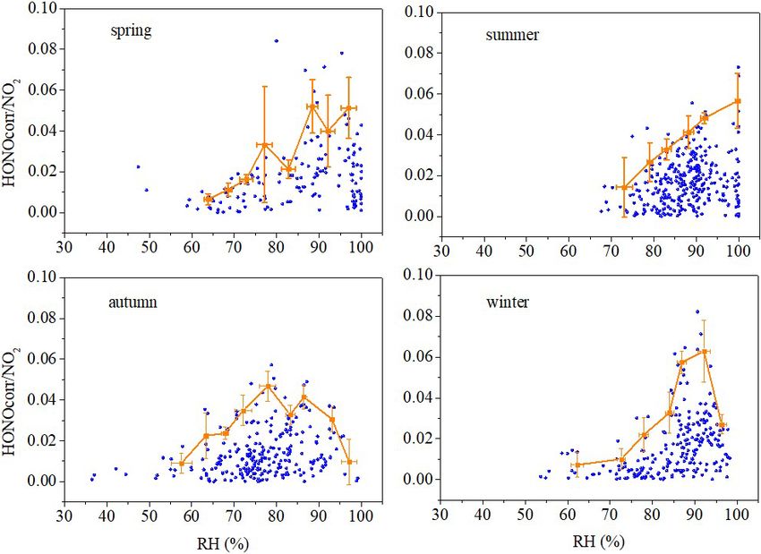
B. Hu et al.: Exploration of the atmospheric chemistry of nitrous acid                                                           377

Figure 3. Diurnal variations in (a) HONO, (b) NO (hollow markers and dashed lines) and NOx (solid markers/lines), (c) HONO / NOx , and
(d) J (NO2 ). The gray shading indicates nighttime (18:00–06:00 LT, including 18:00 LT).

20.07 ppb in autumn, each occurring in the morning rush              value indicates a high HONO production efficiency, which
hour at 10:00, 09:00, 08:00, and 07:00 LT, respectively. Af-         cannot be ascribed to NO2 conversion due to the weak cor-
ter these peaks, NOx decreased during the day in each sea-           relation between HONO and NO2 in summer. Furthermore,
son, probably due to photochemical transformation and in-            high HONO / NO2 ratios were accompanied by high J (NO2 )
creasing boundary-layer depth. The NOx concentrations then           in summer, which indicates that HONO formation during the
began to rise from their minima of 8.20 ppb in summer,               daytime is more likely to relate to light rather than Reac-
8.85 ppb in autumn, 18.10 ppb in winter, and 23.09 ppb in            tion (R5).
spring after 14:00, 13:00, 15:00, and 16:00 LT, respectively,
                                                                                           surf
which was caused by a combination of weak photochemical              NO2 + NO2 + H2 O −→ HONO + HNO3                             (R5)
transformation and reduction in the boundary-layer depth.
The NOx concentrations during winter and spring were sig-            However, the observed maxima can also be ascribed to
nificantly higher than those during autumn and summer. Both          sources independent from NOx concentration, such as soil
the maxima and minima of NOx appeared later in spring and            emissions (Su et al., 2011) and photolysis of particulate ni-
winter compared with summer and autumn.                              trate (Zhou et al., 2011; Ye et al., 2016), which are not in-
   It is possible to better describe the behavior of HONO us-        fluenced by the decrease in NOx concentration around noon.
ing the HONO / NOx ratio. The higher HONO / NOx ratio                A more specific discussion of daytime HONO sources con-
found at noon in the different seasons, especially in summer         sidering the photolysis of particulate nitrate will be given in
and autumn (Fig. 3c), indicates an additional daytime HONO           Sect. 3.4.3. The HONO emissions from soil were estimated
source (Liu et al., 2019a; Xu et al., 2015). It is worth noting      to be 2–5 ppb h−1 (Su et al., 2011). However, soil emission
that the maximum value of this ratio in summer (0.147) was           was a negligible source of HONO in this study since the sur-
significantly higher than the maximum in other seasons, es-          rounding soil is not used for agriculture, and this greatly re-
pecially in winter (0.034). Figure 3d shows that the value           duces the amount of HONO released due to the lack of a
of the HONO / NOx ratio increased with the photolysis rate           fertilization process (Su et al., 2011).
constant of NO2 in summer and autumn, suggesting that the
additional HONO source is probably correlated with light
(Xu et al., 2015; Wang et al., 2017; D. Li et al., 2018; Li
et al., 2012). The increase in the HONO / NO2 ratio dur-
ing the day can be seen more clearly in Fig. 4, and its high

https://doi.org/10.5194/acp-22-371-2022                                                 Atmos. Chem. Phys., 22, 371–393, 2022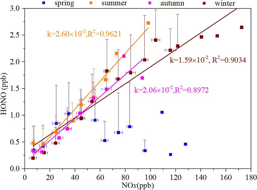
378                                                    B. Hu et al.: Exploration of the atmospheric chemistry of nitrous acid

Figure 4. Scatter plots of NO2 versus HONO color coded by J (NO2 ). The three dashed lines represent 10 %, 5 %, and 1 % ratios of
HONO / NO2 . Daytime was 06:00–18:00 LT, including 06:00 LT.

3.2   Direct vehicle emission of HONO                              from 0.64 to 0.92. The obtained 1HONO / 1NOx ratios (the
                                                                   linear slope of HONO with NOx ) ranged from 0.24 % to
                                                                   2.95 %, with an average value (±SD) of (1.45 ± 0.78) %.
The K+ levels were 0.26, 0.13, 0.14, and 0.24 µg m−3 for
                                                                   These 1HONO / 1NOx ratios have comparability to those
spring, summer, autumn, and winter, respectively. The K+
                                                                   obtained in Guangzhou (1.4 %, Qin et al., 2009; 1.8 %, Li et
levels during the four seasons were lower than 2 µg m−3 ,
                                                                   al., 2012) and Houston (1.7 %, Rappenglück et al., 2013) but
which indicated that biomass burning has little effect on
                                                                   are significantly higher than those measured in Jinan (0.53 %,
this site (Xu et al., 2019). Hence, only vehicle emis-
                                                                   D. Li et al., 2018) and Santiago (0.8 %, Elshorbany et al.,
sions were considered in this study. The consistent diur-
                                                                   2009). The types of vehicle engine, the use of catalytic con-
nal variations in HONO and NOx presented in Sect. 3.1
                                                                   verters, and different fuels will affect the vehicle emission
(Fig. 3) also indicate HONO emissions from local traffic.
                                                                   factors (Kurtenbacha et al., 2001). A potential reason for the
Five criteria were applied to choose cases that guaranteed
                                                                   relatively higher 1HONO / 1NOx values in our study is that
the presence of fresh plumes (Xu et al., 2015; Liu et al.,
                                                                   heavy-duty diesel vehicles pass by on the surrounding high-
2019a): (1) UV < 10 W m−2 ; (2) short-duration air masses
                                                                   way (Rappenglück et al., 2013). It is necessary to examine
(< 2 h); (3) HONO correlating well with NOx (R 2 > 0.60,
                                                                   the specific vehicle emission factors in target cities because
P < 0.05); (4) NOx > 20 ppb (highest 25 % of NOx value);
                                                                   of these differences in 1HONO / 1NOx ratios. Roughly as-
and (5) 1NO / 1NOx > 0.85. A total of 23 cases met these
                                                                   suming that NOx mainly arises from vehicle emissions, a
strict criteria for estimation of the HONO vehicle emission
                                                                   mean 1HONO / 1NOx value of 1.45 % was used as the
ratios. The slopes of scatter plots of HONO vs. NOx were
                                                                   emission factor in this study, and this value was adopted to
used as the emission factors.
                                                                   estimate the contribution of vehicle emissions Pemis to the
   A total of 23 vehicle emission plumes were summarized
                                                                   HONO concentration using
in Table 2, and these were used for estimation of the ve-
hicle emission ratios. These plumes were considered to be          Pemis = NOx × 0.0145.                                      (1)
truly fresh because the mean 1NO / 1NOx ratio (the lin-
ear slope of NO with NOx ) of the selected air masses was          We can then obtain the corrected HONO concentration
99 %. Vehicle plumes unavoidably mixing with other air             (HONOcorr ) for further analysis from the equation
masses resulted in the correlation coefficients (R 2 ) between
HONO and NOx varying among the cases, and these ranged             HONOcorr = HONO − Pemis .                                  (2)

Atmos. Chem. Phys., 22, 371–393, 2022                                                https://doi.org/10.5194/acp-22-371-2022
B. Hu et al.: Exploration of the atmospheric chemistry of nitrous acid                                                            379

                                                                        (1.50, Sörgel et al., 2011), Beijing (0.80; Wang et al., 2017),
                                                                        the eastern Bohai Sea (1.80 % h−1 , Wen et al., 2019), and
3.3     Nighttime heterogeneous conversion of NO2 to                    Kathmandu (1.40 % h−1 , Yu et al., 2009), but more than the
        HONO                                                            value obtained in Shandong (0.29 % h−1 , Wang et al., 2015).
                                                                                       C
                                                                        The highest CHONO      was found in summer, with a value of
3.3.1    Conversion rate of NO2 to HONO                                          −1
                                                                        0.55 % h , which will be explained in Sect. 3.3.2. Another
                                                                        study also found that the highest CHONOC     (1.00 % h−1 ) ap-
Nighttime HONOcorr concentrations can be estimated from
the heterogeneous conversion reaction (Meusel et al., 2016;             peared in summer (Wang et al., 2017).
Alicke, 2002; Su et al., 2008a). Although the mechanism of
the nighttime HONO heterogeneous reaction is unclear, the               3.3.2   The influence factors on HONO formation
                                             0
formula for the heterogeneous conversion (CHONO   ) of NO2
to HONO can be expressed as                                             The hydrolysis of NO2 on wet surfaces producing HONO is
                                                                        first-order affected by the concentration of NO2 (Finlayson-
 0          [HONOcorr ]t2 − [HONOcorr ]t1                               Pitts et al., 2003; Jenkin et al., 1988) and the absorption of
CHONO =                                          ,               (3)    water on the surfaces (Finlayson-Pitts et al., 2003; Kleffmann
                   (t2 − t1 ) × [NO2 ]
                                                                        et al., 1998). A scatter plot of HONOcorr / NO2 vs. RH is
where [NO2 ] is the mean value of NO2 concentration be-                 shown in Fig. 5. We calculated the top-five HONOcorr / NO2
tween t1 and t2 . Equation (4) has been suggested as a way to           ratios in every 5 % RH interval based on a method introduced
avoid the interference of direct emissions and diffusion (Su            in previous literature (Li et al., 2012; Stutz et al., 2004),
et al., 2008a):                                                         which will reduce the influence of those circumstances such
              [HONO ]                                                 as advection, the time of the night, and the surface density.
                        corr (t2 )      [HONOcorr ](t1 )
                                    −                         [X]       These averaged maxima and standard deviations are shown
  X                [X]t2                     [X](t1 )
CHONO    =                                                              in Fig. 5 as orange squares, except where data were sparse in
                                               [NO2 ] t
                           [NO ]
            (t2 − t1 ) 12 [X](t )2 + [X] ( 1 ) [X]
                                    2 (t )
                                                                        a particular 5 % RH interval.
                                      2               (t1 )
               [HONO ]                                                   As for autumn and winter, the influence of RH on
                         corr (t2 )        [HONOcorr ](t1 )
            2       [X]t2            −        [X](t1 )
                                                                        HONOcorr / NO2 can be divided into two parts. The RH pro-
         =                [NO ]              [NO2 ](t )
                                                             ,   (4)   moted an increase in HONOcorr / NO2 for RH values less
                                   2 (t2 )
             (t2 − t1 ) [X](t ) + [X] 1                                 than 77.96 % in autumn and 91.99 % in winter, which is
                             2           (t1 )
                                                                        in line with the reaction kinetics of Reaction (R5). How-
where [HONOcorr ]t , [NO2 ]t , and [X]t were the concentra-             ever, RH inhibits the conversion of NO2 to HONO when
tions of HONO, NO2 , and species used for normalization                 RH is higher than a turning point. According to many pre-
(including NO2 , CO, and black carbon in this study), respec-           vious studies, water droplets will be formed on the surface of
tively, at time t; X is the average concentration of reference          the ground or of aerosols when RH exceeds a certain value,
species between t1 and t2 ; and CHONOX     represents the con-          thus resulting in a negative dependence of HONOcorr / NO2
version rate normalized against reference species X (Su et              on RH (He et al., 2006; Zhou et al., 2007). A similar phe-
al., 2008a). There were 86 cases meeting the criteria. Such a           nomenon was also found in Guangzhou and in Shanghai
large number of cases contributes to the statistical analysis of        (70 %, Li et al., 2012; Wang et al., 2013) and in Kath-
the heterogeneity of HONO formation. The average values                 mandu and in Beijing (65 %, Yu et al., 2009; Wang et al.,
      0          NO2     CO , and C BC                      −1
of CHONO     , CHONO , CHONO           HONO were 0.48 % h ,             2017). However, in summer, RH appeared to promote the
          −1           −1                −1
0.46 % h , 0.46 % h , and 0.46 % h , respectively. The                  increase in HONOcorr / NO2 without a turning point, sug-
combined CHONO C     was 0.46 % h−1 . The average CHONO val-            gesting that HONO production at night in summer strongly
ues obtained using different normalization methods agreed               depends on RH. Another study also found a similar phe-
well. Therefore, an estimation value of 0.46 % h−1 should               nomenon in the summer in Guangzhou (Qin et al., 2009).
be suitable for the nighttime conversion rate from NO2 to               This phenomenon might be caused by water droplets being
HONO.                                                                   evaporated by high temperatures. This is the reason for the
   We also compared the conversion rates calculated in this                         C
                                                                        highest CHONO     in summer. As for spring, the relationship
study with other experiments. As shown in Table 3, CHONO  C             between HONOcorr / NO2 and RH is very complicated and
                                −1             −1
varied widely, from 0.29 % h to 2.40 % h , which may                    needs to be explored further in the future.
be due to the various kinds of land surface in the vari-                   It has been found that NH3 promoted hydrolysis of
ous environments. The CHONO C     in Xiamen is comparable to            NO2 and production of HONO and NH4 NO3 (Xu et al.,
those derived in Shanghai (0.70 % h−1 ; Wang et al., 2013),             2019; L. Li et al., 2018). The correlations between the
Jinan (0.68 % h−1 , D. Li et al., 2018), and Hong Kong                  HONOcorr / NO2 ratio, the NO−      3 / NO2 ratio, and the NH3
(0.52 % h−1 , Xu et al., 2015), less than the values calcu-             concentration in four seasons were examined to investigate
lated from most other sites, including Xinken (1.60 % h−1 ,             the influence of NH3 on HONO formation through pro-
Su et al., 2008a)), Guangzhou (2.40, Li et al., 2012), Spain            moting hydrolysis of NO2 . Only nighttime data with RH

https://doi.org/10.5194/acp-22-371-2022                                                   Atmos. Chem. Phys., 22, 371–393, 2022
380                                                       B. Hu et al.: Exploration of the atmospheric chemistry of nitrous acid

Table 2. Emission ratios of fresh vehicle plumes 1HONO / 1NOx .

                          Date             Time           1NO / 1NOx           R2    1HONO / 1NOx (%)
                          (yyyy/mm/dd)
                          2018/8/1         07:00–08:55            1.1621    0.6897                     2.17
                          2018/8/8         05:40–05:55            0.8727    0.8023                     2.69
                          2018/8/21        05:00–05:55            0.8571    0.7553                     1.14
                          2018/8/31        23:35–23:55            1.1861    0.8130                     1.18
                          2018/10/23       01:05–01:25            0.9893    0.6566                     1.27
                          2018/12/4        07:20–07:40            0.9594    0.8502                     1.11
                          2018/12/10       11:00–11:15            0.8778    0.6735                     1.79
                          2018/12/11       00:00–00:50            0.9424    0.6972                     0.58
                          2018/12/11       04:00–04:55            0.9652    0.7686                     2.12
                          2018/12/11       05:45–06:35            1.0243    0.6566                     0.84
                          2018/12/11       06:40–07:40            0.9992    0.7067                     1.59
                          2018/12/20       22:50–23:10            0.9811    0.7736                     0.97
                          2018/12/21       00:45–01:15            1.0029    0.8914                     1.54
                          2018/12/22       06:40–07:35            1.0194    0.7010                     2.36
                          2018/12/22       07:40–08:05            0.9932    0.7831                     2.94
                          2018/12/25       21:00–22:10            0.9573    0.8857                     1.64
                          2018/12/26       03:50–04:15             1.167    0.6540                     1.39
                          2018/12/26       06:45–07:45            0.9971    0.8463                     0.92
                          2018/12/26       07:55–08:25            0.9714    0.6919                     2.95
                          2018/12/27       04:50–05:30            0.9365    0.7265                     0.76
                          2019/3/6         07:30–08:05            1.0309    0.8283                     0.74
                          2019/3/9         07:50–08:05            0.9933    0.9203                     0.24
                          2019/3/9         12:00–12:55            0.9627    0.6444                     0.51

Figure 5. Scatter plots of nighttime HONOcorr / NO2 ratios versus RH. The average top-five HONOcorr / NO2 in every 5 % RH interval are
shown as orange squares, and the error bars show ±1 SD.

Atmos. Chem. Phys., 22, 371–393, 2022                                                   https://doi.org/10.5194/acp-22-371-2022
B. Hu et al.: Exploration of the atmospheric chemistry of nitrous acid 381
Table 3. Overview of the conversion frequencies from NO2 to HONO in Xiamen and comparisons with other studies.
Location Date Conversion rate Reference
(% h−1 )
Xiamen, China Aug 2018–Mar 2019 0.46 This study
Mar 2019 (spring) 0.46
Aug 2018 (summer) 0.55
Oct 2018 (autumn) 0.44
Dec 2018 (winter) 0.37
Xinken, China Oct–Nov 2004 1.60 Su et al. (2008b)
Jinan, China Sep 2015–Aug 2016 0.68 D. Li et al. (2018)
Mar–May 2016 (spring) 0.43
Jun–Aug 2016 (summer) 0.69
Sep–Nov 2015 (autumn) 0.75
Dec 2015–Feb 2016 (winter) 0.83
Guangzhou, China Jun 2006 2.40 Li et al. (2012)
Spain Nov–Dec 2008 1.50 Sörgel et al. (2011)
Beijing, China Sep 2015–July 2016 0.80 Wang et al. (2017)
Apr–May 2016 (spring) 0.50
Jun–Jul 2016 (summer) 1.00
Sep–Oct 2015 (autumn) 0.90
Jan 2016 (winter) 0.60
Shandong, China Nov 2013–Jan 2014 0.29 Wang et al. (2015)
Shanghai, China Aug 2010–Jun 2012 0.70 Wang et al. (2013)
Eastern Bohai Sea, China Oct–Nov. 2016 1.80 Wen et al. (2019)
Hong Kong, China Aug 2011–May 2012 0.52 Xu et al. (2015)
Kathmandu, Nepal Jan–Feb 2003 1.4 Yu et al. (2009)
above 80 % were chosen to avoid daytime rapid photoly- NO2 hydrolysis and HONO production in winter. All in all,
sis of HONO and enough water for NO2 quick hydrolysis NH3 might promote NO2 hydrolysis and HONO production
(Xu et al., 2019). As shown in Fig. 6, for summer, the cor- in spring and winter, whereas NH3 played a minor role in
relations between NH3 and the HONOcorr / NO2 ratio was HONO production in summer and autumn.
very poor and even negative (R = −0.0438), and the corre- As shown in Fig. S3, HONOcorr / NO2 reached a pseudo-
lation between the NO− 3 / NO2 ratio and NH3 was also neg- steady state from 03:00 to 06:00 LT every night. A corre-
ative (−0.2908). These results indicated that NH3 played a lation analysis of HONOcorr / NO2 with PM2.5 was carried
minor role in HONO production in summer. For autumn, out in the pseudo-steady state to understand the impact of
although the NO− 3 / NO2 ratio correlated well with NH3 aerosols on HONO production. Although we did not mea-
(R = 0.3965) in autumn, the HONOcorr / NO2 ratio had a sure the aerosol surface density, the aerosol mass concen-
negative correlation with NH3 (R = −0.1305), which also tration can be used to replace this parameter (Huang et al.,
indicated that NH3 played a minor role in HONO produc- 2017; Park et al., 2004; Cui et al., 2018). The positive cor-
tion in autumn. For spring, the correlation coefficient be- relation of HONOcorr with PM2.5 (R1 = 0.4987) (Fig. 7a)
tween the HONOcorr / NO2 ratio and the NH3 concentration may be a result of atmospheric physical processes such as
was the highest among the four seasons (0.3662), and the convergence and diffusion. Using the HONOcorr / NO2 ratio
correlation between the NO− 3 / NO2 ratio and the NH3 con- instead of a single HONO concentration for correlation anal-
centration was positive (0.1716). These phenomena proved ysis with PM2.5 reduced the impact of physical processes and
that NH3 might promote HONO and NH4 NO3 production indicated the extent of conversion of NO2 to HONO. There-
through promoting NO2 hydrolysis in spring. For winter, fore, it was more credible that HONOcorr / NO2 would be
positive correlations were found between NH3 and both moderately positively correlated with PM2.5 (R2 = 0.2331)
the HONO / NO2 ratio (R = 0.1718) and NO− 3 / NO2 ra- during the whole observation period (Fig. 7b). As denoted
tio (R = 0.2543), which indicated that NH3 might promote by larger green squares in the Fig. 7b, HONOcorr / NO2 cor-
https://doi.org/10.5194/acp-22-371-2022 Atmos. Chem. Phys., 22, 371–393, 2022382 B. Hu et al.: Exploration of the atmospheric chemistry of nitrous acid
Figure 6. The correlation between the NH3 concentration and HONO / NO2 ratio (upper) and the correlation between the NH3 concentration
and NO−
3 / NO2 (lower) in four seasons. The scatter points were colored by ambient RH values.
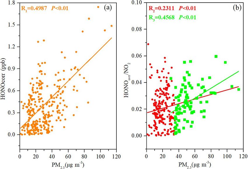
Atmos. Chem. Phys., 22, 371–393, 2022 https://doi.org/10.5194/acp-22-371-2022B. Hu et al.: Exploration of the atmospheric chemistry of nitrous acid 383
related well with PM2.5 when its concentration was higher of the next interval, and this accounts for changes in con-
than 35 µg m−3 (R3 = 0.4568). The larger the amount of centration levels (Sörgel et al., 2011). The parameter Ldep
HONO produced by the heterogeneous reaction of NO2 can be quantified by multiplying the dry deposition rate of
on the aerosol surface, the better the correlation between HONO by the observed HONO concentration
and then di-
ground
HONO / NO2 and PM2.5 (Cui et al., 2018; Wang et al., 2003; νHONO ×[HONO]
viding by the mixing layer height Ldep = H .
Hou et al., 2016; Li et al., 2012; Nie et al., 2015).
ground
A value of νHONO = 2 cm s−1 was used for the deposition
3.4 Daytime sources of HONO rate (Sörgel et al., 2011; Su et al., 2008a). Although the mix-
ing layer heights during spring, summer, autumn, and win-
3.4.1 Budget analysis of HONO
ter were 1074.4, 1173.8, 1494.6, and 1310.4 m, respectively
Having discussed the nighttime chemical behavior of (Gao, 1999), most HONO cannot reach the height of 200 m
HONO, we now concentrate on the daytime chemical behav- due to rapid photolysis of HONO during the daytime. There-
ior of HONO. Here, Runknown is used to stand for the rate fore, the mixing layer height 200 m was used to parameter-
of emission from unknown sources. The value of Runknown ize Ldep . In summarizing the known HONO sources, we in-
was estimated based on the balance between sources and cluded the nighttime heterogeneous production as a known
sinks due to its short atmospheric lifetime. The sources are source based on the assumption that the day continues in the
(1) oxidation of NO by OH (ROH+NO = kOH+NO [NO][OH]), same way as the night (Sörgel et al., 2011). The term Phete
(2) dark heterogeneous production (Phet ), and (3) direct ve- was parameterized by NO2 conversion at night using the for-
C
mula Phete = CHONO [NO2 ] (Alicke, 2002).
hicle emission (Pemis ); the sinks are (1) HONO photolysis
(Rphot = JHONO [HONO]), (2) oxidation of HONO by OH Figure 8 shows the contributions of each term in Eq. (7) to
(ROH+HONO = kOH+HONO [HONO][OH]), and (3) dry depo- the HONO budgets in different seasons. Photolysis of HONO
sition (Ldep ). The value of Runknown can then be calculated (Rphot ) formed the largest proportion of the sinks in all
according to four seasons, accounting for 87.85 %, 88.79 %, 88.15 %, and
86.71 % in spring, summer, autumn, and winter, respectively.
Runknown = JHONO [HONO] + kOH+HONO [HONO][OH] The value of Rphot in summer was the highest (3.60 ppb h−1 ),
1[HONO] followed by spring (3.08 ppb h−1 ), autumn (2.38 ppb h−1 ),
+ Ldep + − kOH+NO [NO][OH] and winter (2.26 ppb h−1 ). The oxidation of HONO by OH
1t
− Phet − Pemis , (5) contributed little to HONO sinks (2.77 % of all sinks). Dry
deposition (Ldep ) was also very small (9.35 % of all sinks).
where kOH+HONO = 6.0 × 10⁻¹² cm3 molecules−1 s−1 and As for known sources, ROH+NO was the main known source
kOH+NO = 7.4 × 10⁻¹² cm3 molecules−1 s−1 , values cited in all four seasons, wherein the largest proportion was found
from a previous study (Sörgel et al., 2011). The OH concen- in summer (64.44 %), followed by autumn (53.66 %), spring
tration ([OH]) was estimated in this study because no data (53.25 %), and winter (51.73 %). Direct emission was second
for this value were available. An improved empirical for- among the known sources, accounting for 38.36 %, 27.49 %,
mula, Eq. (6), was applied to estimate [OH] using the NO2 37.02 %, and 40.81 % in spring, summer, autumn, and winter,
and HONO concentrations and the photolysis rate constants respectively. Dark heterogeneous formation (Phete ) was al-
(J ) of NO2 , O3 , and HONO (Wen et al., 2019). Equation (6) most negligible in the daytime, accounting for approximately
fully considers the influence of photolysis and precursors on 8.31 % of known sources during the whole observation pe-
the concentration of [OH]. riod. As for unknown sources, these made up the largest pro-
portion of all sources found in summer (81.25 %), followed
[OH] = 4.1 × 10⁹ by autumn (73.99 %), spring (70.87 %) and winter (59.28 %).
J (O1 D)0.83 × J (NO2 )0.19 × (140 × NO2 + 1) It is worth noting that Runknown exhibited a maximum
+HONO × J (HONO) around noon in all seasons. A previous study in Wangdu (Liu
× (6)
0.41 × NO22 + 1.7 × NO2 + 1 + NO × kNO+OH et al., 2019b) also found that unknown sources of HONO
+HONO × kHONO+OH reached a maximum at midday, with the strongest photol-
ysis rates in summer. This strengthens the validity of the
During spring, summer, autumn, and winter, the average assumption that the missing HONO formation mechanism
midday OH concentrations were 8.86 × 10⁶ , 1.48 × 10⁷ , is related to a photolytic source (Michoud et al., 2014). In
1.36 × 10⁷ , and 6.19 × 106 cm−3 , respectively, which were the present study, the daily maximum Runknown value was
within the range of those obtained in other studies varying 4.51 ppb h−1 in summer, followed by 3.51 ppb h−1 in spring,
from 4 × 10⁶ to 1.7 × 107 cm−3 (Tan et al., 2017; Lu et al., 3.28 ppb h−1 in autumn, and 2.08 ppb h−1 in winter. Aver-
2013). age Runknown during the whole observation was 2.32 ppb h−1 ,
1[HONO]
1t is the observed change of HONO concentration which was almost at the upper–middle level of studies re-
(ppb s−1 ). The value of 1[HONO]
1t is the concentration differ- ported: 0.5 ppb h−1 in a forest near Jülich, Germany (Kleff-
ence between the center of one interval (1 min) and the center
https://doi.org/10.5194/acp-22-371-2022 Atmos. Chem. Phys., 22, 371–393, 2022384 B. Hu et al.: Exploration of the atmospheric chemistry of nitrous acid Figure 7. The correlation between PM2.5 and HONOcorr (a) and the correlation between PM2.5 and HONOcorr / NO2 (b). The squares depict PM2.5 ≥ 35 µg m−3 ; all scattered points are from the time when the ratio of HONOcorr / NO2 reached a pseudo-steady state each night (03:00–06:00 LT). Figure 8. Average diurnal variations of each source (> 0) and sink (< 0) of HONO in the four seasons. Atmos. Chem. Phys., 22, 371–393, 2022 https://doi.org/10.5194/acp-22-371-2022
B. Hu et al.: Exploration of the atmospheric chemistry of nitrous acid                                                        385

mann, 2005); 0.77 ppb h−1 at a rural site in the Pearl River        summer (Zhou et al., 2007; Li et al., 2012; Wang et al., 2017)
delta, China (Li et al., 2012); 1.04 ppb h−1 at a suburban site     using
in Nanjing, China (Liu et al., 2019a); ≈ 2 ppb h−1 in Xinken,                               Runknown × H
China (Su et al., 2008a); and 2.95 ppb h−1 in the urban atmo-       JNO− →HONO =                               ,               (7)
                                                                          3            f × [NO−3 ] × υNO− × td
sphere of Jinan, China (D. Li et al., 2018).                                                             3

                                                                    where JNO− →HONO is the rate of photolysis of NO−
                                                                                                                    3 to form
                                                                                  3
3.4.2   Exploration of possible unknown daytime sources             HONO, υNO− is the dry deposition rate of NO−     3 during the
                                                                                  3
According to the analyses in Sects. 3.1 and 3.4.1, the un-          period td , and f is the proportion of the surface exposed
known sources are likely to be related to light. It was in-         to the sun at midday. Here, we suppose that the surfaces
deed found that the unknown sources have a good corre-              involving NO−   3 were exposed to light by a factor f = 1/4,
lation with the parameters related to light. It was reported        taking mixing height H = 200 m and υNO− = 5 cm s−1
                                                                                                                    3
in previous studies that particulate nitrate photolysis is a        over td = 24 h. We use the mean midday value of
source of HONO (Ye et al., 2017, 2016; Scharko et al.,              Runknown = 9.72 µg m−3 h−1 and [NO−       3 ] = 10.35 µg m
                                                                                                                               −3

                                                                    in     spring     and                          −3
                                                                                             Runknown = 11.51 µg m h   −1    and
2014; Romer et al., 2018; McFall et al., 2018). We will
discuss the possibility of HONO being produced by pho-              [NO− 3 ] = 2.86  µg m −3 in summer. The photolysis rates

tolysis of particulate nitrate (J (NO3 _R) × pNO−                   JNO− →HONO derived from Eq. (8) were 4.83 × 10⁻⁵ s−1 and
                                                      3 ) at this         3
site in this section. There was a logarithmic relationship          2.07 × 10⁻⁴ s−1 for spring and summer, respectively. These
showing good correlation between Runknown (ppb h−1 ) and            values were in the range 6.2 × 10⁻⁶ to 5.0 × 10⁻⁴ obtained
J (NO−                −
       3 _R) × pNO3 (µg m
                              −3 s−1 ) in spring (R 2 = 0.6519)
                                                                    in a previous study (Ye et al., 2017), which indicated that
                   2
and summer (R = 0.6511), while relatively weak cor-                 particulate nitrate photolysis could be a likely source for the
relation was found in autumn (R 2 = 0.3633) and win-                missing daytime additional HONO formation in spring and
ter (R 2 = 0.4186) (Fig. 9). This result indicated that pho-        summer. The variability of JNO− →HONO may be caused by
                                                                                                     3
tolysis of particulate nitrate contributed more in spring           chemical composition, acidity, light-absorbing constituents,
and summer than in autumn and winter. In conditions of              and the optical and other physical properties of aerosols.
relatively lower J (NO3 _R) × pNO−      3 , Runknown increased
rapidly with increasing pNO−     3 concentration and its pho-       3.5       Parameterization of HONO
tolysis rate constant but reached a plateau after a criti-
cal value (J (NO3 _R) × pNO−     3 > 0.5 µg m
                                                −3 s−1 in sum-      Through an empirical parameterized formula, we can ex-
mer, J (NO3 _R) × pNO−    3 >  0.4 µg m −3 s−1 in autumn, and       plore an accurate parameterization method for HONO, dis-
J (NO3 _R) × pNO−    3 > 1.5 µg m
                                  −3 s−1 in winter). There was      cuss the main control factors for the HONO concentration
no obvious turning point in spring, but it could be seen that       and its chemical behavior, and quantify its main sources
the growth rate was declining. This indicated that in condi-        and key kinetic parameters. As mentioned in Sect. 3.1, the
tions that were relatively cleaner, the missing daytime source      HONO / NOx ratio is better than HONO / NO2 as an indi-
of HONO was limited by the pNO−        3 concentration and the      cator of HONO generation. In another study (Elshorbany et
photolysis rate constant. However, with enough particulate          al., 2012), data were collected from 15 field observations
nitrate providing sufficient precursor or enough light to stim-     all over the world to establish the correlation between the
ulate the reaction, the HONO production did not increase            HONO / NOx ratio and the HONO concentration in global
as J (NO3 _R) × pNO−    3 increased. Other generation mecha-        models. Therefore, we applied this method in this study to
nisms might play leading roles in the condition with enough         parameterize the HONO concentration. As shown in Fig. 10,
particulate nitrate or enough light. It was found in a previ-       the 1HONO / 1NOx ratios in the four seasons were close
ous study that heterogeneous soot photochemistry may con-           to the calculated value (0.02). However, there were sea-
tribute to the daytime HONO concentration (Monge et al.,            sonal variations in the slope, showing a maximum in sum-
2010). Black carbon (BC) values were used as a substitute           mer (2.60 × 10⁻² ), followed by autumn (2.06 × 10⁻² ), and
for soot values (Sörgel et al., 2011). When BC concentration        a minimum in winter (1.59 × 10⁻² ). Except for in spring,
was above 2.0 µg m−3 , the missing daytime source of HONO           HONO showed good correlation with NOx , with R 2 values
did not increase as J (NO3 _R) × pNO−    3 increased. We found      ranging from 0.8972 to 0.9621. Therefore, we used slopes
that the missing daytime source of HONO correlated bet-             of 2.60 × 10⁻² , 2.06 × 10⁻² , and 1.59 × 10⁻² to parameter-
ter with BC × UV (R = 0.9269, R = 0.6356) than with BC              ize the HONO concentrations in summer, autumn, and win-
(R = 0.4776, R = 0.6071) or UV (R = 0.8494, R = 0.4262)             ter, respectively. As for spring, though only a weak corre-
alone in autumn and winter (Fig. S4), probably related to the       lation between HONO and NOx was found, the majority of
conversion of NO2 to HONO on BC enhanced by light.                  the 1HONO / 1NOx ratios fluctuated round a slope of 0.02
   We discuss whether photolysis of particulate nitrate was         because concentrations of NOx greater than 60 ppb only ac-
able to provide enough additional HONO by estimating the            counted for 8.83 % of the data. Therefore, a slope of 0.02 was
rate of HONO production by nitrate photolysis in spring and         applied in spring to parameterize the HONO concentration.

https://doi.org/10.5194/acp-22-371-2022                                                 Atmos. Chem. Phys., 22, 371–393, 2022
You can also read