Variability and extremes: statistical validation of the Alfred Wegener Institute Earth System Model (AWI-ESM)
←
→
Page content transcription
If your browser does not render page correctly, please read the page content below
Geosci. Model Dev., 15, 1803–1820, 2022
https://doi.org/10.5194/gmd-15-1803-2022
© Author(s) 2022. This work is distributed under
the Creative Commons Attribution 4.0 License.

Variability and extremes: statistical validation of the Alfred
Wegener Institute Earth System Model (AWI-ESM)
Justus Contzen1,2 , Thorsten Dickhaus3 , and Gerrit Lohmann1,2
1 Alfred  Wegener Institute, Helmholtz Centre for Polar Marine Research, Bremerhaven, Germany
2 Department    of Environmental Physics, University of Bremen, Bremen, Germany
3 Institute for Statistics, University of Bremen, Bremen, Germany

Correspondence: Justus Contzen (justus.contzen@awi.de)

Received: 28 June 2021 – Discussion started: 29 July 2021
Revised: 21 December 2021 – Accepted: 28 January 2022 – Published: 3 March 2022

Abstract. Coupled general circulation models are of               ison of empirical cumulative distribution functions. These
paramount importance to quantitatively assessing the magni-       analyses can also be conducted over seasonal and annual
tude of future climate change. Usual methods for validating       averages (climatologies) or along latitudinal and longitudi-
climate models include the evaluation of mean values and          nal transects (Tapiador et al., 2012). The comparison of cli-
covariances, but less attention is directed to the evaluation     mate indices is also common in model validation (Sillmann
of extremal behaviour. This is a problem because many se-         et al., 2013; Zhang et al., 2011). While climate models are
vere consequences of climate change are due to climate ex-        able to reproduce many climate phenomena across the globe,
tremes. We present a method for model validation in terms         their reliability regarding extremes requires additional eval-
of extreme values based on classical extreme value theory.        uation. Changes in the intensity and frequency of extremes
We further discuss a clustering algorithm to detect spatial de-   have drawn much attention during recent decades (IPCC,
pendencies and tendencies for concurrent extremes. To illus-      2012; Rahmstorf and Coumou, 2011; Horton et al., 2016),
trate these methods, we analyse precipitation extremes of the     mainly due to their large impacts on the natural environment,
Alfred Wegener Institute Earth System Model (AWI-ESM)             economy and human health (Ciais et al., 2005; Kovats and
global climate model and from other models that take part         Kristie, 2006). For instance, the summer heatwave over Cen-
in the Coupled Model Intercomparison Project CMIP6 and            tral Europe in 2003 resulted in extensive forest fires, crop
compare them to the reanalysis data set CRU TS4.04. The           yield reductions and fatalities (de Bono et al., 2004; Vanden-
clustering algorithm presented here can be used to determine      torren et al., 2004). During the 20th and early 21st century,
regions of the climate system that are then subjected to a fur-   the frequency of high-temperature extremes increased in Eu-
ther in-depth analysis, and there may also be applications in     rope (Dong et al., 2017), even after the apparent levelling off
palaeoclimatology.                                                of global mean temperatures after 2000 (Trenberth and Fa-
                                                                  sullo, 2013), and a similar development has been observed
                                                                  for precipitation extremes (Fischer and Knutti, 2016). Due to
                                                                  the inherent nature of extreme events, their evolution differs
1   Introduction                                                  from that of the mean and the variance (Schär et al., 2004;
                                                                  IPCC, 2012) and also depends on the strength of the events
Coupled general circulation models are frequently utilised        themselves (Myhre et al., 2019).
to quantitatively assess the magnitude of future climate             In particular, the concurrent occurrence of climate ex-
change. Validating these models by simulating different cli-      tremes at different locations may have especially large im-
mate states is essential for understanding the sensitivity of     pacts on agriculture (Toreti et al., 2019), human societies and
the climate system to both natural and anthropogenic forc-        economies (Jongman et al., 2014), and the climate system it-
ing. Usual methods for validating climate models include the      self (Zscheischler et al., 2014). Large-scale climate extremes
evaluation of mean values and covariances and the compar-

Published by Copernicus Publications on behalf of the European Geosciences Union.
1804                                      J. Contzen et al.: Variability and extremes: statistical validation of the AWI-ESM

can furthermore cause serious problems for insurance and            The resulting clusters for model and observational data are
reinsurance companies (Mills, 2005). For these reasons, an          compared and used to analyse the ability of the climate model
increasing amount of research is being conducted on multi-          to reproduce spatial dependencies of precipitation extremes.
variate analysis of extremes with a focus on their concurrent          In this article, our main focus is on the AWI-ESM, and
appearance (Shaby and Reich, 2012; Dombry et al., 2018;             we present our methods using data from this model. We also
Kornhuber et al., 2020; Ionita et al., 2021a), and new tools        present a measure for the model accuracy in regard to ex-
have been created for the analysis of extremes in climate           tremal precipitation and apply it to a set of different CMIP6
models (Weigel et al., 2021).                                       models. In the main text, results will be discussed for the
    A particular challenge for the analysis of extreme events       AWI-ESM and for the model identified as having the best
is the fact that extreme events are typically rare and that it is   model accuracy. In the Supplement to this paper, the results
therefore difficult to build informative statistics based solely    for the other CMIP6 models investigated are presented.
on the extreme events themselves. Two common approaches                Model validation in terms of precipitation extremes is al-
are used to overcome this issue: peaks over threshold and           ready an active research topic. Tabari et al. (2016) investi-
block maxima. In the peaks-over-threshold approach, a fixed         gate the performance of global and regional climate models
threshold is selected. The distribution of the data exceed-         using the peaks-over-threshold approach. An evaluation of
ing this threshold can then be approximated by a generalised        regional and global climate models using extreme precipita-
Pareto distribution if some additional assumptions are ful-         tion indices is conducted by Bador et al. (2020), revealing a
filled (see McNeil et al., 2015, chap. 7.2, for more details).      tendency for stronger extremes in regional models. A similar
The peaks-over-threshold approach is frequently applied in          result was obtained by Mahajan et al. (2015) by comparing
climatology and hydrology (Acero et al., 2011; Fowler and           climate model and observational precipitation data over the
Kilsby, 2003; Kiriliouk et al., 2019). The block-maxima ap-         United States using GEV distributions. Timmermans et al.
proach, on the other hand, follows the idea of splitting the        (2019) conduct pairwise comparisons of the precipitation ex-
time axis into blocks of a sufficiently large size and inves-       tremes of numerous gridded observation-based data sets and
tigating the block-wise maxima of the data. Under suitable          find considerable differences between the data sets, espe-
conditions, the distribution of these block-wise maxima can         cially in mountainous regions. Precipitation extremes over
be approximated by a generalised extreme value (GEV) dis-           India are investigated by Mishra et al. (2014) using GEV
tribution for large sample sizes.                                   distributions and comparisons of indices with a focus on
    In this work, we will evaluate the performance of the           changes over time.
fully coupled Alfred Wegener Institute Earth System Model              It is also not a new approach to apply clustering algorithms
(AWI-ESM1.1LR) (Shi et al., 2020; Lohmann et al., 2020;             to climate data. For example, it has been used to define cli-
Ackermann et al., 2020) in terms of its accuracy regarding          mate zones in the United States (Fovell and Fovell, 1993) and
variability and extremes of precipitation, putting special fo-      globally (Zscheischler et al., 2012) and to find regions with
cus on spatially concurrent precipitation extremes. Our main        similar trends in their climatic change over Europe (Carvalho
questions are whether the model is able to accurately repro-        et al., 2016). Those analyses focus on mean values and on
duce extreme events in different regions and whether spatial        their temporal differences, respectively, while we apply clus-
dependencies and concurrent extremal events are modelled            tering specifically to uncover connections regarding climate
adequately. We compare model data from a historical run of          extremes.
the AWI-ESM to the global precipitation reanalysis data set            The article is structured as follows. After introducing the
CRU TS4.04 (Harris et al., 2020b). We start with investigat-        data sets in Sect. 2, we present the methods used in Sect. 3.
ing variability and extremes locally using empirical statisti-      The results from their application to the data are presented
cal parameters and by fitting a GEV distribution to annual          in Sect. 4. A section on conclusions and discussions finalises
precipitation maxima. Afterwards, following an approach by          the article.
Bernard et al. (2013), we use a clustering algorithm to group
spatio-temporal climate data into different spatial regions
based on their similarity in terms of extremal behaviour and        2   Data
the concurrency of their extremes. This clustering is based
on the theory of max-stable copulae, which has been used            The observational data are reanalysed monthly precipitation
in prior work to investigate spatial dependence of extreme          data in mm over land (excluding Antarctica) from the CRU
precipitation events, for example in Bargaoui and Bárdossy          TS4.04 data set (Harris et al., 2020b; University of East An-
(2015); Zhang et al. (2013); Qian et al. (2018). In those pa-       glia Climatic Research Unit, 2020) with data ranging from
pers, an analysis of bivariate distributions is performed. In       1901 to 2019. We restrict the timeframe to the years 1930
our work, we first construct for each pair of locations a mea-      to 2014 in order to have a sufficiently large area with non-
sure for their similarity in terms of extremes. This measure is     missing data and to be consistent with the climate model
then used as a basis for the clustering algorithm to group the      data. The grid size is 0.5 × 0.5◦ , and the data have been ob-
data into spatial regions of comparable extremal behaviour.         tained by interpolating observations from more than 4000

Geosci. Model Dev., 15, 1803–1820, 2022                                             https://doi.org/10.5194/gmd-15-1803-2022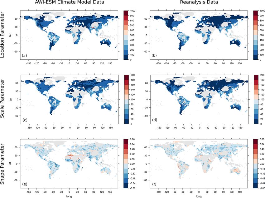
J. Contzen et al.: Variability and extremes: statistical validation of the AWI-ESM 1805
weather stations using angular distance weighting. At some by the Earth System Grid Federation (ESGF; Cinquini et al.,
locations and time points, no data from nearby weather sta- 2014).
tions were available to use for interpolation. In these cases, In our analysis, we restrict the timeframe of the model
the creators of the CRU TS4.04 data set used a value from data to the years 1930 to 2014, as in the observational data.
a climatology instead. These climatology values are not very We investigate monthly precipitation (the sum of convective
informative in terms of extremes and using too many of them precipitation and large-scale precipitation) in millimetres per
would distort the analyses; therefore, all grid points with month. We use bilinear interpolation to scale the reanalysis
more than 5 % climatology values and all grid points with data to the grid of the atmospheric component of the cli-
at least 12 consecutive months of climatology values are ex- mate model and take into account only those interpolated
cluded from our analysis. This results in the exclusions of grid points that correspond to locations with given observed
large regions in northern and central Africa, Indonesia, cen- data, excluding the oceans and the regions with incomplete
tral Asia, and at the poles. In the figures showing geographi- data mentioned above.
cal data in this paper, these regions are coloured in grey. The
climate model used is the coupled model AWI-ESM1.1LR.
It is based on the AWI Earth System Model (AWI-ESM1), 3 Methods
which consists of the AWI Climate Model (Sidorenko et al.,
3.1 Univariate analysis
2015; Rackow et al., 2018), but with interactive vegetation.
The model is comprised of the atmosphere model ECHAM6 In this subsection, the time series of each spatial location
(Stevens et al., 2013), which is run with the T63L47 setup (henceforth referred to as grid point) is investigated sepa-
(i.e. a horizontal resolution of 1.85 × 1.85◦ and 47 verti- rately, and all operations and analyses described are therefore
cal layers) and the ocean–sea ice model FESOM1.4 (Wang conducted for each grid point. Since the focus of this work is
et al., 2014), which employs an unstructured grid, allowing not on evaluating the effects of longtime trends, we apply a
for varying resolutions from 20 km around Greenland and seasonal–trend decomposition using Loess (Cleveland et al.,
in the North Atlantic to around 150 km in the open ocean 1990) on the data and subtract the trend from the data but add
(CORE2 mesh). The land surface processes are computed by the mean value of the trend, resulting in data for which we
the land surface model JSBACH2.11 (Reick et al., 2013). The assume temporal stationarity. Following this, as a first com-
model considers the surface runoff toward the coasts, deploy- parison between the data sets, we investigate differences in
ing a hydrological discharge model that also includes fresh- the empirical mean and empirical standard deviation of the
water fluxes by snowmelt (Hagemann and Dümenil, 1997). annually maximised precipitation data.
AWI-ESM1 has been extensively used and described in the The theoretical foundation for the application of the
context of palaeoclimate changes and changes in the recent GEV distribution is as follows. For a random variable X
and future climate (Shi et al., 2020; Lohmann et al., 2020; with an unknown probability distribution, we investigate
Ackermann et al., 2020; Niu et al., 2021). The historical run the distribution of the maximum of independent and iden-
is documented in Danek et al. (2020) and has been directly tically distributed (i.i.d.) copies X1 , . . ., Xn of it: Y (n) :=
used in Ackermann et al. (2020) and Keeble et al. (2021). maxi=1,...,n (Xi ). We assume that for suitable normalising se-
Furthermore, the model takes part in CMIP6/PMIP4 activi- quences an >0 and bn , Y (n) converges in distribution if n
ties (Brierley et al., 2020; Brown et al., 2020; Otto-Bliesner tends to infinity:
et al., 2021; Kageyama et al., 2021a, b).
The Coupled Model Intercomparison Project (CMIP), Y (n) − bn D
coordinated by the Working Group on Coupled Mod- → H.
− (1)
an
elling (WGCM) of the World Climate Research Programme
(WCRP) has the goal of supporting and facilitating the anal- In this case, as shown by Fréchet (1927), Fisher and Tippett
ysis of climate model data by providing a set of common (1928), and Gnedenko (1943), the distribution of Y (n) can be
standards regarding the formatting and availability of model approximated by a GEV distribution for a large (fixed) value
output. Additionally, in order to enhance model comparabil- of n. This distribution depends on three parameters, called
ity, all models participating in CMIP are required to run a set location (µ), scale (σ >0) and shape (γ ), and its cumulative
of standardised experimental setups (Diagnostic, Evaluation distribution function is given by
and Characterization of Klima experiments; DECK experi- x−µ
exp − exp − σ γ =0
ments) and a simulation of the historical climate from 1850 Fµ,σ,γ (x) = − 1 (2)
exp −max 0, 1 + γ x−µ
γ
to 2014 (the historical simulations we also use in our analy- σ γ 6= 0.
sis). CMIP is divided into different phases, reflecting the ad-
vancements of climate modelling; the current phase (CMIP6) The GEV distribution has widely been used as a model for
started in 2016. More information on CMIP can be found in block-wise maximised data (for example, Coles et al., 2003;
Eyring et al. (2016). The model outputs are made available Onwuegbuche et al., 2019; Villarini et al., 2011). Follow-
ing this approach, we group our monthly precipitation data
https://doi.org/10.5194/gmd-15-1803-2022 Geosci. Model Dev., 15, 1803–1820, 2022
1806                                      J. Contzen et al.: Variability and extremes: statistical validation of the AWI-ESM

from observations and climate model into 1-year block max-          quantiles. Using these notations, we define
ima and fit a GEV distribution to the block-wise maxima at                      1 X
each grid point. When selecting a block size, a bias–variance       AWQD :=            cos (lat(g)) ·
                                                                               |G| g∈G
tradeoff has to be taken into account. For a low block size,
the resulting parameter estimates tend to be biased because                      q̂0.95,mod (g) − q̂0.95,obs (g) .                  (3)
the convergence to the GEV distribution holds only asymp-
totically. A high block size, on the other hand, will lead to a     3.2   Comparison of spatial distributions
limited amount of block-wise maxima that can be analysed
and therefore to a higher variance in the estimates (see Mc-        To compare the spatial distributions of climate extremes,
Neil et al., 2015, chap. 7). In our case, we have a relatively      we introduce a hierarchical clustering algorithm (using av-
small block size of 12 (months per year) and 90 block-wise          erage linking) to determine regions with similar extremal
maxima (years of investigation).                                    behaviour. This approach is similar to the idea proposed in
   To estimate the distribution parameters, we use the method       Bernard et al. (2013). The hierarchical clustering is based on
of probability-weighted moments developed by Hosking                concepts from extreme value statistics that will be discussed
(1985) as implemented in the R package “EnvStats” of Mil-           in the following.
lard and Kowarik (2013). As shown by Hosking et al. (1985),            Assume that two real-valued random variables (X, Y )
this method yields estimators with a relatively low variance        have a copula function C: [0,1] × [0,1] → [0,1], mean-
and bias compared to the maximum likelihood approach, es-           ing that their joint distribution function can be written in
pecially for small- and medium-sized samples. We test the           terms of the copula and the marginal distribution functions
goodness of fit using a one-sample Kolmogorov–Smirnov               as FX,Y (x, y) = C(FX (x), FY (y)) for all x, y ∈ R. Thus, if
(KS) test at a 5 % significance level. The null hypothesis of       (X, Y ) is the weak limit of block-wise maxima of a sequence
the test is that the annually maximised data follow the GEV         of i.i.d. two-dimensional variables when the block size goes
distribution having the probability-weighted moments esti-          to infinity (a similar condition as in Sect. 3.1 but extended to
mates as distribution parameters.                                   two-dimensional random variables), it follows that X and Y
   We also use the parametric bootstrap method with 2500            are (jointly) GEV distributed. It also follows that the copula
resamples to compute 95 % confidence intervals for each             must fulfil C(ut , v t ) = C t (u, v) for all u, v ∈ [0, 1] and t>0
GEV parameter and for the 95 % quantiles of the distribu-           (see McNeil et al., 2015, Theorem 7.44 and 7.45). Such a
tions. Confidence intervals for the GEV parameters based on         copula is called max-stable, and it can be written as follows:
asymptotic normality also exist for the probability-weighted

                                                                                                                 ln u
moments estimators, but they have a high bias and variance          C(u, v) = exp (ln u + ln v) AX,Y                         ,       (4)
                                                                                                             ln u + ln v
if the shape parameter is far away from zero, as shown by
Hosking et al. (1985). In our data, such a value is estimated       which uses a function AX,Y : [0,1] → [ 21 , 1] called
for the shape parameter for several time series, and compar-        the Pickands dependence function (Pickands, 1981). The
isons between the confidence intervals based on bootstrap           function AX,Y is convex and satisfies max(w, 1 − w) ≤
and those based on asymptotic normality also confirmed              AX,Y (w) ≤ 1 for all w ∈ [0, 1]. The extremal coefficient is
large differences in these cases. For the sake of methodolog-       now defined as 2 times its value at the point 0.5:
ical consistency (and because we also use the bootstrap for         θX,Y := 2 · AX,Y (0.5).                                         (5)
the confidence intervals of the 95 % quantiles), we calculated
the GEV parameter confidence intervals using bootstrap for          The extremal coefficient takes its minimal possible value of
all time series. Since this method is quite time-consuming, it      1 if X and Y are comonotonic (meaning specifically that it
could also be appropriate to choose the method of confidence        holds θX,X = 1 for all X). The maximal possible value of
interval calculation based on the estimated shape parameter         2 is obtained if X and Y are stochastically independent. To
value.                                                              estimate the extremal coefficient, we use the madogram esti-
   To compare the performance of different CMIP6 models,            mator as described in Ribatet et al. (2015) and Cooley et al.
we introduce average weighted quantile difference (AWQD)            (2006) and rewrite θX,Y as
as a measure for the accuracy of the extremal precipitation.                  1 + 2νX,Y
For this measure, the absolute differences between model            θX,Y =              ,                                           (6)
                                                                              1 − 2νX,Y
and observational 95 % GEV quantiles, weighted with the co-
sine of the latitude, are averaged. The weighting accounts for      with the madogram νX,Y = 21 E[|FX (X) − FY (Y )|]. The
the fact that the grid cells do not have an equal size for all      madogram can be estimated by replacing FX and FY
grid points, and the average is taken because of the different      with their empirical counterparts. For a data sample
model resolutions. Let G denote the set of grid points. For         (x1 , y1 ), . . ., (xn , yn ), we then obtain
g ∈ G, let q̂0.95,mod (g) and q̂0.95,obs (g) denote the estimated                        n X  n
                                                                                  1     X
                                                                    ν̂X,Y =                     (1x ≤x − 1yj ≤yi ) ,                (7)
                                                                              2n(n + 1) i=1 j =1 j i

Geosci. Model Dev., 15, 1803–1820, 2022                                               https://doi.org/10.5194/gmd-15-1803-2022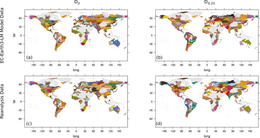
J. Contzen et al.: Variability and extremes: statistical validation of the AWI-ESM                                                 1807

and consequently define an estimator                                  Chan (2004) is to find a point from which on the growth
                                                                      rate of the dissimilarity measure increases considerably. It
          1 + 2ν̂X,Y                                                  can then be expected that the clusters up to this point com-
θ̂X,Y =              .                                         (8)
          1 − 2ν̂X,Y                                                  bine rather similar data points, whereas combining the data
                                                                      points to larger clusters would yield artificial results. To de-
Hierarchical clustering algorithms require a dissimilar-              termine such a point of change, first a suitable range of the
ity function D : G × G → R that must fulfil D(g1 , g2 ) =             number of clusters is selected. For our example, we consider
D(g2 , g1 ) ≥ 0 and D(g1 , g1 ) = 0 for all grid points g1 , g2 ∈     different ranges, starting with 10 clusters and having no more
G (for an introduction to hierarchical clustering algorithms,         than 550 clusters. For each possible point of change c in this
see Murtagh and Contreras, 2012). Based on the properties             range, the horizontal axis of the graph is divided into the two
of the extremal coefficient discussed above, we define such a         parts to the left and the right of that point, and a linear regres-
dissimilarity function as follows:                                    sion line is fitted to each of the two partial graphs. The root-
                                                                      mean-squared errors (RMSEs) of the two regression lines are
D0 (g1 , g2 ) := θ̂X,Y − 1,                                    (9)
                                                                      weighted with the number of points involved in the regres-
with X and Y representing the GEV distributions at the grid           sion analysis and summed up. The point of change with the
points g1 and g2 , respectively.                                      minimal combined RMSE is chosen as the suitable cluster
   Note that the extremal coefficient is invariant under rank         number. As an alternative method, we set the number of clus-
transformations and that it does not depend on the values of          ters to the highest possible number such that a fixed thresh-
the GEV parameters of the marginal distributions. In fact, in         old dissimilarity between clusters is not exceeded (threshold
Ribatet et al. (2015); Cooley et al. (2006), it was only used         method). This number can easily be read off of the evaluation
in the special case of margins following a GEV(1, 1, 1) dis-          graph.
tribution. It may be desirable to also include the dissimilarity
of the marginal distributions in the clustering. As a further
generalised dissimilarity measure we propose                          4   Results

                                                                      We start with calculating the empirical mean and standard

                                             1
Dλ (g1 , g2 ) := (1 − λ) D0 (g1 , g2 ) + λ     dµ (g1 , g2 ) +        deviation of the annually maximised data for each grid point,
                                             3
                                                                     as can be seen in Fig. 1. In most regions, similar mean val-
                  1                1
                    dσ (g1 , g2 ) + dγ (g1 , g2 ) ,            (10)   ues can be observed. A notable overestimation of the annual
                  3                3                                  maxima of monthly precipitation by the climate model takes
                                                                      place in the Himalayas and along the western coasts of the
where λ ∈ [0, 1] is a weighting parameter and dµ (g1 , g2 ) :=
     |µ̂g1 −µ̂g2 |                                                    Americas. Underestimation occurs most prominently in the
                     ∈ [0, 1] is the normalised distance be-
maxh1 ,h2 ∈G |µ̂h1 −µ̂h2 |                                            Amazon region and parts of Central America, as well as in
tween the location parameter estimates at the grid points g1          Bangladesh and East Asia. Looking at the standard devia-
and g2 (analogous for dσ and dγ ). Instead of an equal weight-        tion, a similar pattern to that of the empirical mean can be
ing, it would also be possible to use different weights for dµ ,      observed, but it has a stronger tendency for underestimation,
dσ and dγ , but the selection of a set of weights that is clearly     which also occurs in India and the northern part of Australia.
better suited to describing GEV distribution dissimilarity is         In Fig. 2a and b, quantile–quantile plots (Q–Q plots) of the
difficult. It could be a good idea to put more weight on the          empirical mean and standard deviation are displayed. The
shape parameter since this parameter describes the heavy-             quantiles of the empirical mean are generally similar, but the
tailedness of the distribution and therefore the strength of          highest quantiles show a strong discrepancy. Regarding the
its extremes relative to the non-extreme values. On the other         standard deviation, this tendency is much more pronounced,
hand, we will see in the next section that the uncertainty in         corresponding to the larger areas of underestimation of em-
the shape parameter estimation is considerably higher than            pirical standard deviation we identified in Fig. 1. The differ-
the uncertainty in the estimation of the other two parameters,        ence in empirical mean and the difference in empirical stan-
at least for our data, which would speak against weighting            dard deviation are plotted against each other in Fig. 2c). It
shape parameter differences too strongly.                             is visible that in many cases overestimation (underestima-
   To choose a suitable number of clusters, we consider an            tion) of the empirical mean also corresponds to overestima-
approach by Salvador and Chan (2004) called the L method.             tion (underestimation) of the empirical standard deviation.
In each step of the hierarchical clustering, the two clusters         A similar case of heteroscedasticity has also been noted in
with minimal dissimilarity are combined; therefore, we can            Lohmann (2018) when investigating Holocene climate.
plot the number of clusters versus the dissimilarity between             As pointed out by Katz and Brown (1992), the frequency
them, resulting in a graph called the evaluation graph. The           of extreme events is strongly influenced by changes (or, in
dissimilarity between clusters necessarily grows as the to-           this case, misestimation) in the mean and in the variance of a
tal number of clusters is reduced. The idea of Salvador and           distribution. Therefore, an overestimation or underestimation

https://doi.org/10.5194/gmd-15-1803-2022                                                 Geosci. Model Dev., 15, 1803–1820, 2022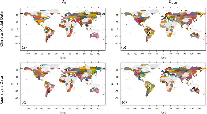
1808                                       J. Contzen et al.: Variability and extremes: statistical validation of the AWI-ESM

Figure 1. The empirical mean (a, c, e) and empirical standard deviation (b, d, f) of the annual maxima of monthly precipitation of the
AWI-ESM model data set (a, b) and the CRU TS4.04 reanalysis data set (c, d) and their difference (model data minus reanalysis data) (e, f).
Values exceeding the scale limits are truncated. Values are given in millimetres per month.

of extremes can be expected in certain regions based on the             can likewise obtain the similarity between the anomalies of
results in Figs. 1 and 2.                                               scale parameters and empirical standard deviations. For the
   When fitting the GEV distributions to the data and apply-            location parameter, we observe large differences quite of-
ing KS tests to check the goodness of fit, the hypothesis that          ten, and the parameters estimated for one data set seldom
the data follow a GEV distribution with the estimated pa-               fall into the confidence interval derived from the other data
rameters is not rejected for almost all grid points in both the         set. The estimated scale parameters are covered more often
observational and climate model data, except for in parts of            by the confidence intervals derived from the other data set,
the Sahara and some isolated points.                                    although there are also large regions with a high difference
   The three GEV parameters estimated are location, scale               in the two estimates. The estimated shape parameters are
and shape, with location and scale very roughly correspond-             covered by the confidence intervals at many locations, but
ing to mean and variance, and the shape parameter yielding              it needs to be noted that the estimator of the shape param-
information about the degree of heavy-tailedness. The esti-             eter is known to be sensitive to small variations in the data.
mated parameter values are shown in Fig. 4. In Fig. 5, the              Therefore, the confidence intervals calculated using the para-
differences between model and observational parameters are              metric bootstrap tend to be large and not particularly infor-
shown. Shaded areas are areas in which the model parameter              mative. In Fig. 6, the anomalies of the 95 % upper quantiles
falls into the 95 % confidence interval of the corresponding            of the estimated GEV distributions are depicted, again with
observation parameter and vice versa. We can observe a sim-             shaded areas indicating quantiles lying within the confidence
ilarity between the anomaly of the location parameters and              levels determined using a parametric bootstrap. Climate ex-
the anomaly of the empirical means discussed above, and we              tremes are most strongly overestimated by the model in the

Geosci. Model Dev., 15, 1803–1820, 2022                                                  https://doi.org/10.5194/gmd-15-1803-2022
J. Contzen et al.: Variability and extremes: statistical validation of the AWI-ESM                                              1809

                                                                     Table 1. The number of clusters for the AWI-ESM climate model
                                                                     and observational data determined with the L Method (m data) and
                                                                     the threshold method (h data) for different ranges and thresholds
                                                                     and for the dissimilarity measures D0 (a) and D0.25 (b).

                                                                                 (a)
                                                                                 D0           AWI-ESM       Observations
                                                                                 m = 250           64            146
                                                                                 m = 300          148            148
                                                                                 m = 400          200            296
                                                                                 m = 500          234            291
                                                                                 h = 0.85         143            127
                                                                                 h = 0.825        188            177
                                                                                 h = 0.8          232            221
                                                                                 h = 0.775        280            254
                                                                                 (b)
                                                                                 D0.25        AWI-ESM       Observations
                                                                                 m = 250          187            102
                                                                                 m = 300          165            142
                                                                                 m = 400          223            140
                                                                                 m = 500          232            265
                                                                                 h = 0.675        118            109
                                                                                 h = 0.65         165            167
                                                                                 h = 0.625        219            220
                                                                                 h = 0.6          281            265

                                                                        The results of the L method seem to depend rather strongly
                                                                     on the data set investigated and the value of m (compare the
                                                                     results for m = 250 and m = 300 for measure D0 ), making
                                                                     this method less suitable for the comparison of two data sets.
Figure 2. Quantile–quantile (Q–Q) plots comparing the empirical
                                                                     The threshold method generally predicts a similar but (in
mean values (a) and the empirical standard deviations (b) of the
annually maximised monthly precipitation of the CRU TS4.04 re-
                                                                     most cases) slightly lower cluster number for observational
analysis data set and the AWI-ESM model data set. The deviance of    data than for climate model data. In Fig. 7, the clusters for
the empirical mean and standard deviation are plotted against each   both data sets are depicted using the threshold method for
other in (c). Values are given in millimetres per month.             dissimilarity measure D0 with threshold h = 0.825 and for
                                                                     dissimilarity measure D0.25 with threshold h = 0.65.
                                                                        To exemplify the differences and similarities in the cluster-
mountainous regions of the Himalayas, the Andes and the              ings, we have a closer look at Europe in the D0 clusterings.
Rocky Mountains. An underestimation of climate extremes              In the model data, there is one cluster covering western Spain
takes place most notably in the Amazon region and parts of           and Portugal, one cluster covering eastern Spain, and one
eastern Asia. This corresponds well to the regions of over-          cluster consisting of southern France and Italy. Great Britain
estimation and underestimation of the empirical means and            and Denmark are in the same cluster, and the northern parts
standard deviations and the implications of such misestima-          of France together with Belgium and the Netherlands are in
tions discussed above.                                               another. One cluster covers Germany and Switzerland, and in
   We apply the hierarchical clustering algorithms using the         eastern Europe we see several clusters covering larger areas
two dissimilarity measures D0 and D0.25 as introduced in the         in a longitudinal direction, e.g. one cluster over Poland, one
previous section. The numbers of clusters determined using           over Ukraine, and one over Turkey and Greece. The clusters
the L method with selected cluster ranges (from 10 to a max-         in the observational data set show a slightly different pic-
imal number of clusters m) and using the threshold method            ture. Here, the whole Iberian Peninsula is in one cluster, and
with selected threshold dissimilarities h are documented in          one large cluster extends over northern France, Belgium, the
Table 1.                                                             Netherlands, Germany and the western parts of Poland. On
                                                                     the other hand, Great Britain and Denmark are now in two
                                                                     separate clusters. Regarding other parts of the world, it is

https://doi.org/10.5194/gmd-15-1803-2022                                                 Geosci. Model Dev., 15, 1803–1820, 2022
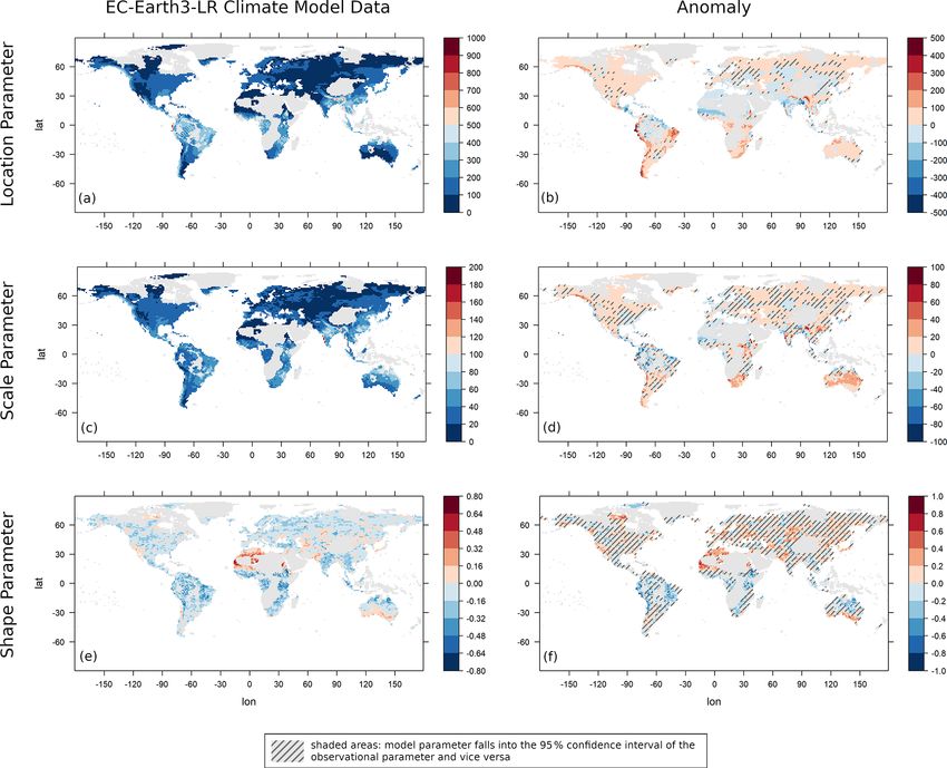
1810                                      J. Contzen et al.: Variability and extremes: statistical validation of the AWI-ESM

Figure 3. The p values of Kolmogorov–Smirnov tests for the hypothesis that the data follow a GEV distribution with parameters estimated
using probability-weighted moments. Test results for the AWI-ESM climate model (a) and for the CRU TS4.04 reanalysis data (b).

Figure 4. The estimated GEV parameters location (a, b), scale (c, d) and shape (e, f) for the AWI-ESM climate model data (a, c, e) and
reanalysis data (b, d, f). Values exceeding the scale limits are truncated. Values are given in millimetres per month.

Geosci. Model Dev., 15, 1803–1820, 2022                                                https://doi.org/10.5194/gmd-15-1803-2022
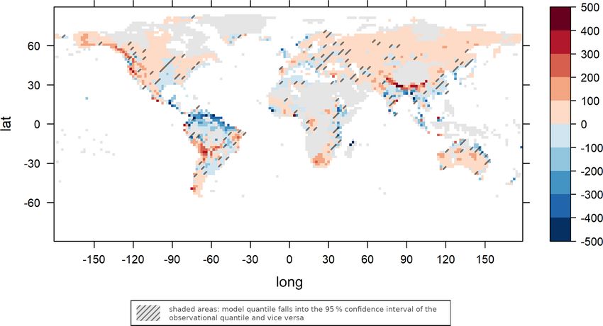
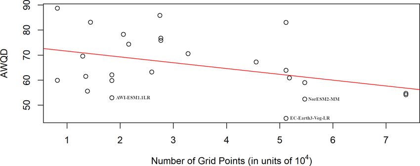
J. Contzen et al.: Variability and extremes: statistical validation of the AWI-ESM                                              1811

Figure 5. Difference between AWI-ESM model and observational GEV parameter estimates: location parameter (a), scale parameter (b) and
shape parameter (c). Values exceeding the scale limits are truncated. Values are given in millimetres per month.

worth noting that in all four clusterings a large cluster cover-     full table of the models and their AWQDs is provided in the
ing the Sahara (or at least all parts of it for which there are      Supplement to this paper. In Fig. 8, the AWQDs are plotted
observations available) can be identified. There are no clus-        against the model resolution (the total number of model grid
ters extending over two regions that are very far apart from         points in units of 104 ). A linear regression (shown as a red
each other, and in general clusters tend to cover more area in       line; intercept: 73.310; slope: −2.368) indicates that models
the longitudinal direction than in the latitudinal one.              with a higher resolution have a tendency to describe extremal
   For the AWI-ESM, we calculated an AWQD of 52.98,                  precipitation better. A test of the significance of the slope pa-
making it the third best of all 27 CMIP6 models analysed. A          rameter (null hypothesis of the slope parameter being equal

https://doi.org/10.5194/gmd-15-1803-2022                                               Geosci. Model Dev., 15, 1803–1820, 2022
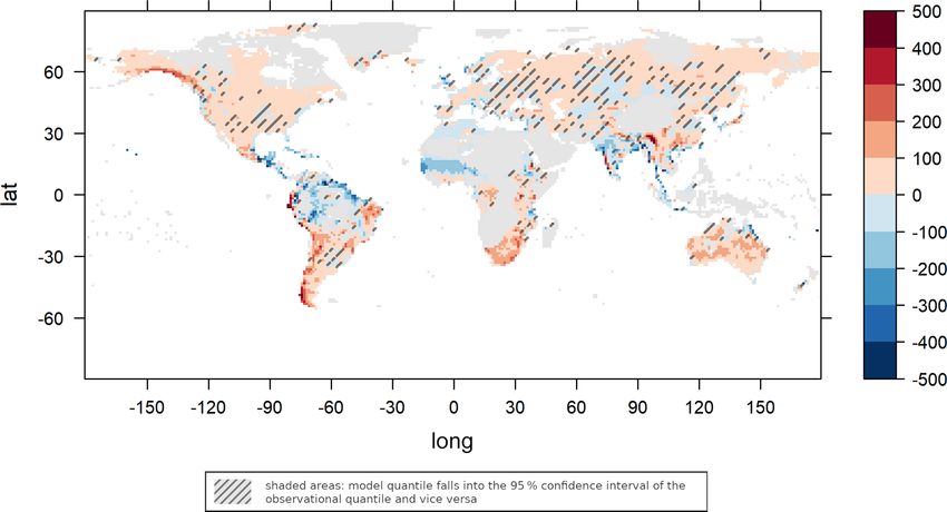
1812                                       J. Contzen et al.: Variability and extremes: statistical validation of the AWI-ESM

Figure 6. Difference between the 0.95 quantiles of the estimated GEV distribution for AWI-ESM model and observational data. Values
exceeding the scale limits are truncated. Values are given in millimetres per month.

Figure 7. Clustering of AWI-ESM model data (a, b) and observational data (c, d) with the dissimilarity measure D0 and threshold h = 0.825
(a, c) and with the dissimilarity measure D0.25 and threshold h = 0.65 (b, d).

to zero) was significant at the 5 % level with a p value of            the estimated GEV parameters and anomalies are shown in
0.0357. The best model in terms of the AWQD is the high-               Fig. 9. The differences in the 95 % quantiles are depicted
resolution model EC-Earth3-Veg-LR (EC-Earth Consortium,                in Fig. 10. The numbers of clusters determined using the
2020) with a value of 44.71. We will now discuss results for           L method and the threshold method are found in Table 2,
this model in more detail, while results for the other models          and images of clusterings are shown in Fig. 11. Q–Q plots
can be found in the Supplement. For the EC-Earth3-Veg-LR,              and plots of KS tests are similar to the corresponding plots

Geosci. Model Dev., 15, 1803–1820, 2022                                                 https://doi.org/10.5194/gmd-15-1803-2022
J. Contzen et al.: Variability and extremes: statistical validation of the AWI-ESM                                                     1813

Figure 8. The average weighted quantile difference (AWQD) of the 27 CMIP6 models considered plotted against the model resolution
(number of model grid points in units of 104 ). The linear regression line (intercept 73.310, slope −2.368) is shown in red.

Figure 9. GEV parameters estimated using the EC-Earth3-Veg-LR climate model (a, c, e) and their anomaly compared to the reanalysis GEV
parameters (b, d, f). The GEV parameters are location (a, b), scale (c, d) and shape (e, f). Values exceeding the scale limits are truncated.
Values are given in millimetres per month.

https://doi.org/10.5194/gmd-15-1803-2022                                                     Geosci. Model Dev., 15, 1803–1820, 2022
1814                                      J. Contzen et al.: Variability and extremes: statistical validation of the AWI-ESM

Figure 10. Difference in the 0.95 quantiles for the estimated GEV distribution from EC-Earth3-Veg-LR model and the observational data.
Values exceeding the scale limits are truncated. Values are given in millimetres per month.

Figure 11. Clustering of the EC-Earth3-Veg-LR model data (a, b) and the observational data (c, d) with the dissimilarity measure D0 and
threshold h = 0.825 (a, c) and with dissimilarity measure D0.25 and threshold h = 0.65 (b, d).

for the AWI-ESM and can be found in the Supplement to                 is in general higher than for the AWI-ESM, in part proba-
this paper. The EC-Earth3-Veg-LR model predicts climate               bly due to the higher model resolution (320 × 160 compared
extremes better than AWI-ESM in the Himalayas and in the              to 192 × 96). Note that this increased resolution is also the
Amazon region (cf. Fig. 6 and 10), while it overestimates             reason for the different values for the cluster numbers of the
precipitation extremes more strongly than the AWI-ESM at              reanalysis data in Tables 1 and 2 because in each case reanal-
the western coast of South America. The number of clusters            ysis data were interpolated to the climate model resolution.

Geosci. Model Dev., 15, 1803–1820, 2022                                                https://doi.org/10.5194/gmd-15-1803-2022
J. Contzen et al.: Variability and extremes: statistical validation of the AWI-ESM                                              1815

Table 2. The number of clusters for the EC-Earth3-Veg-LR climate      we can also identify larger regions of overestimation and un-
model and the observational data determined with the L method (m      derestimation of empirical means and standard deviations by
data) and the threshold method (h data) for different ranges and      the climate model. These misestimations often go hand in
thresholds and for the dissimilarity measures D0 (a) and D0.25 (b).   hand with a similar misestimation of the standard deviation
                                                                      (heteroscedasticity), but for the standard deviation a stronger
        (a)                                                           tendency for underestimation can be observed. Misestima-
        D0            EC-Earth3-Veg-LR       Observations             tions of mean and standard deviations translate into a mises-
        m = 250                76                89                   timation of extreme values, and this can be confirmed by the
        m = 300               141                 90                  comparison of the fitted GEV distribution parameters and the
        m = 400               181                 94                  0.95 quantiles derived from them. The shape parameter, in-
        m = 500               184                272                  dicative of the heavy-tailedness of the distribution, is in gen-
        h = 0.85              173                145                  eral similar between model and observational data, but be-
        h = 0.825             224                186                  cause of the difficulties in reliably estimating this parameter
        h = 0.8               299                240                  from data (that are in turn a result of the rareness of extreme
        h = 0.775             366                272                  events in the data), these results have to be taken with cau-
                                                                      tion.
        (b)
        D0.25         EC-Earth3-Veg-LR       Observations                The cluster analysis based on spatial dependencies and the
                                                                      occurrence of concurrent extremes shows that there is gener-
        m = 250               113                 67                  ally a good agreement between identified clusters. The num-
        m = 300               117                 67                  ber of clusters is also similar in general, with a slight ten-
        m = 400               129                154
                                                                      dency for a higher cluster number in the model data. Since
        m = 500               146                282
                                                                      it is mostly large-scale weather events and teleconnections
        h = 0.675             131                116                  contributing to concurrent climate extremes, this may indi-
        h = 0.65              203                166                  cate that the basic physical behaviour underlying them is in
        h = 0.625             276                225                  general well captured by the AWI-ESM. Further analyses can
        h = 0.6               358                279                  be conducted to investigate the reasons for different cluster-
                                                                      ings over selected regions in detail.
                                                                         In addition to the AWI-ESM, several other CMIP6 mod-
When again comparing the clusters over Europe using the D0            els are also analysed. A comparison of the model accuracy,
dissimilarity measure, it can be observed that in the western         measured using an averaged quantile difference, shows a ten-
part of Europe model and observational clusters are similar in        dency for higher-dimensional models to capture extremal be-
general, with only slight differences over the Iberian Penin-         haviour better.
sula and with an area covering southern France and northern              In this work, a clustering algorithm based on bivariate ex-
Italy that is in one cluster in the model data and in two dif-        tremal coefficients is used to perform a spatial analysis of
ferent clusters in the observational data. In eastern Europe          extreme values. Extremal coefficients are also used to model
and Scandinavia, the differences between the clusterings are          multivariate spatial distributions of extremal precipitation us-
larger, and thus it is more difficult to see correspondences.         ing max-stable processes. This method was first developed
The general remarks that have been made about the cluster-            by Smith (1990) and Schlather (2002) and was then extended
ings while discussing the AWI-ESM data also apply here.               by Opitz (2013) and Ribatet et al. (2015), and it has been used
                                                                      successfully to model precipitation over Switzerland (Rib-
                                                                      atet, 2017). The models based on max-stable processes as-
5   Conclusions                                                       sume spatial stationarity (i.e. the spatial dependence between
                                                                      two points depends only on their distance). This assump-
We presented approaches and methods to validate climate               tion is justifiable for small regions like Switzerland, but it
model outputs by comparing their extremal behaviour to the            makes the models in their present form unsuitable for global
extremal behaviour of observational data. To illustrate these         data. Castro-Camilo and Huser (2020) created a model for
methods, we compared precipitation extremes between the               the spatial distributions of extreme tail dependencies based
AWI-ESM and the CRU TS4.04 data set of reanalysed ob-                 on factor copulae, allowing them to use the relaxed assump-
servations. After an analysis of empirical statistical parame-        tion of local spatial stationarity and therefore to apply their
ters, we fitted the data to GEV distributions and analysed the        model to the whole contiguous United States. From the area
differences in estimated parameters. Following this, we con-          of parametric copulae, vine copulae have also been employed
tinued with an analysis of spatial concurrence of extremes            to model precipitation data by Vernieuwe et al. (2015) and
based on a hierarchical clustering approach and a dissimilar-         by Nazeri Tahroudi et al. (2021). A further possibility is the
ity measure derived from bivariate copula theory. While the           application of non-parametric multivariate copulae. Marcon
empirical statistics are similar for many parts of the world,         et al. (2014) used an estimator based on Bernstein polyno-

https://doi.org/10.5194/gmd-15-1803-2022                                                Geosci. Model Dev., 15, 1803–1820, 2022
1816 J. Contzen et al.: Variability and extremes: statistical validation of the AWI-ESM
mials to model the common distribution of up to seven vari- Competing interests. The contact author has declared that neither
ables in their analysis of French precipitation data. Copulae they nor their co-authors have any competing interests.
based on Bernstein polynomials are also used in multivariate
extreme value analysis with a focus on multiple testing (Neu-
mann et al., 2019). In global climate models, the number of Disclaimer. Publisher’s note: Copernicus Publications remains
dimensions is much higher than seven, and thus the method neutral with regard to jurisdictional claims in published maps and
by Marcon et al. (2014) is not directly transferable. institutional affiliations.
The clustering approach presented here focuses on the
comparison of extremal events at different locations, thereby
Acknowledgements. The authors are grateful to Manfred Mudelsee
supplementing the analyses of climate extremes that are of-
for constructive discussions and helpful suggestions. The authors
ten focused on extremes at a specific location (Zhang et al., also would like to thank GMD editor Julia Hargreaves and the edi-
2011). An application to daily data that has been annually torial team, as well as the reviewers Anna Kiriliouk and Qingxiang
or seasonally maximised is also possible but is beyond the Li, for their useful and constructive feedback. We acknowledge the
scope of this paper. In order to investigate extreme precipita- World Climate Research Programme, which, through its Working
tion within the area covered by one cluster in more detail, Group on Coupled Modelling, coordinated and promoted CMIP6.
the spatially stationary max-stable models or the copulae- We thank the climate modelling groups for producing and mak-
based models mentioned above could be employed. Most of ing available their model output, the Earth System Grid Federation
the clusters cover only a small region, therefore spatial sta- (ESGF) for archiving the data and providing access to them, and the
tionarity might be a reasonable assumption, although it is not multiple funding agencies that support CMIP6 and ESGF.
a direct consequence of the data being in the same cluster. In
addition to model validation, the definition of regions with
concurrent extremes may turn out to be useful for assess- Financial support. Justus Contzen is funded through the
Helmholtz School for Marine Data Science (MarDATA) (grant
ments of risks in an economical context and for insurance. It
no. HIDSS-0005). Gerrit Lohmann receives funding through
needs to be noted, however, that extremes in climate models “Ocean and Cryosphere under climate change” in the Program
and in gridded reanalysis data sets tend to be damped because “Changing Earth – Sustaining our Future” of the Helmholtz Society
of the spatial averaging performed during the creation of the and PalMod through the Bundesministerium für Bildung und
data (Bador et al., 2020). Another possible field of applica- Forschung (grant no. 01LP1917A).
tion is palaeoclimatology. The spatial distribution of precip-
itation extremes is known to have changed markedly in the The article processing charges for this open-access
past (Lohmann et al., 2020; Ionita et al., 2021b), and cluster- publication were covered by the Alfred Wegener Institute,
ing based on climate models could be used to generalise the Helmholtz Centre for Polar and Marine Research (AWI).
sparse existing palaeoclimatic data to larger regions.
Review statement. This paper was edited by Julia Hargreaves and
Code and data availability. The CRU TS4.04 reanaly- reviewed by Qingxiang Li and Anna Kiriliouk.
sis data are available at https://catalogue.ceda.ac.uk/uuid/
89e1e34ec3554dc98594a5732622bce9 (Harris et al., 2020a).
The AWI-ESM climate model data are available under
https://doi.org/10.22033/ESGF/CMIP6.9328 (Danek et al.,
2020), and the EC-Earth3-Veg-LR model data can be found References
under https://doi.org/10.22033/ESGF/CMIP6.4702 (EC-Earth
Consortium, 2021). The software code (in R) used for the analyses Acero, F. J., García, J. A., and Gallego, M. C.: Peaks-
is provided in the Supplement to this paper. over-Threshold Study of Trends in Extreme Rainfall
over the Iberian Peninsula, J. Climate, 24, 1089–1105,
https://doi.org/10.1175/2010JCLI3627.1, 2011.
Supplement. The supplement related to this article is available on- Ackermann, L., Danek, C., Gierz, P., and Lohmann, G.: AMOC
line at: https://doi.org/10.5194/gmd-15-1803-2022-supplement. Recovery in a Multicentennial Scenario Using a Coupled
Atmosphere-Ocean-Ice Sheet Model, Geophys. Res. Lett., 47,
e2019GL086810, https://doi.org/10.1029/2019GL086810, 2020.
Bador, M., Boé, J., Terray, L., Alexander, L. V., Baker, A., Bel-
Author contributions. The initial concept was created by TD and
lucci, A., Haarsma, R., Koenigk, T., Moine, M.-P., Lohmann,
GL. JC led the writing of the paper and implemented the statisti-
K., Putrasahan, D. A., Roberts, C., Roberts, M., Scoccimarro,
cal data diagnostics. TD contributed to statistical methodology. GL
E., Schiemann, R., Seddon, J., Senan, R., Valcke, S., and
contributed to the climatological analysis. All authors read and ap-
Vanniere, B.: Impact of Higher Spatial Atmospheric Reso-
proved the manuscript.
lution on Precipitation Extremes Over Land in Global Cli-
mate Models, J. Geophys. Res.-Atmos., 125, e2019JD032184,
https://doi.org/10.1029/2019JD032184, 2020a.
Geosci. Model Dev., 15, 1803–1820, 2022 https://doi.org/10.5194/gmd-15-1803-2022J. Contzen et al.: Variability and extremes: statistical validation of the AWI-ESM 1817 Bargaoui, Z. and Bárdossy, A.: Modeling short duration extreme Coles, S., Pericchi, L. R., and Sisson, S.: A fully probabilistic ap- precipitation patterns using copula and generalized maximum proach to extreme rainfall modeling, J. Hydrol., 273, 35–50, pseudo-likelihood estimation with censoring, Adv. Water Re- https://doi.org/10.1016/S0022-1694(02)00353-0, 2003. sour., 84, 1–13, https://doi.org/10.1016/j.advwatres.2015.07.006, Cooley, D., Naveau, P., and Poncet, P.: Variograms for spatial 2015. max-stable random fields, in: Dependence in Probability and Bernard, E., Naveau, P., Vrac, M., and Mestre, O.: Clustering of Statistics, edited by: Bertail, P., Soulier, P., and Doukhan, P., Maxima: Spatial Dependencies among Heavy Rainfall in France, Springer, New York, 373–390, https://doi.org/10.1007/0-387- J. Climate, 26, 7929–7937, https://doi.org/10.1175/JCLI-D-12- 36062-X, 2006. 00836.1, 2013. Danek, C., Shi, X., Stepanek, C., Yang, H., Barbi, D., Brierley, C. M., Zhao, A., Harrison, S. P., Braconnot, P., Williams, Hegewald, J., and Lohmann, G.: AWI AWI-ESM1.1LR C. J. R., Thornalley, D. J. R., Shi, X., Peterschmitt, J.-Y., Ohgaito, model output prepared for CMIP6 CMIP historical, Ver- R., Kaufman, D. S., Kageyama, M., Hargreaves, J. C., Erb, M. sion 20200212, Earth System Grid Federation [data set]„ P., Emile-Geay, J., D’Agostino, R., Chandan, D., Carré, M., https://doi.org/10.22033/ESGF/CMIP6.9328, 2020. Bartlein, P. J., Zheng, W., Zhang, Z., Zhang, Q., Yang, H., de Bono, A., Giuliani, G., Kluser, S., and Peduzzi, P.: Impacts of Volodin, E. M., Tomas, R. A., Routson, C., Peltier, W. R., Otto- summer 2003 heat wave in Europe, UNEP/DEWA/GRID, Europ. Bliesner, B., Morozova, P. A., McKay, N. P., Lohmann, G., Environ. Alert. Bull., 2, 1–4, 2004. Legrande, A. N., Guo, C., Cao, J., Brady, E., Annan, J. D., Dombry, C., Ribatet, M., and Stoev, S.: Probabilities of Con- and Abe-Ouchi, A.: Large-scale features and evaluation of the current Extremes, J. Am. Stat. Assoc., 113, 1565–1582, PMIP4-CMIP6 midHolocene simulations, Clim. Past, 16, 1847– https://doi.org/10.1080/01621459.2017.1356318, 2018. 1872, https://doi.org/10.5194/cp-16-1847-2020, 2020. Dong, B., Sutton, R. T., and Shaffrey, L.: Understanding the rapid Brown, J. R., Brierley, C. M., An, S.-I., Guarino, M.-V., Steven- summer warming and changes in temperature extremes since the son, S., Williams, C. J. R., Zhang, Q., Zhao, A., Abe-Ouchi, mid-1990s over Western Europe, Clim. Dynam., 48, 1537–1554, A., Braconnot, P., Brady, E. C., Chandan, D., D’Agostino, https://doi.org/10.1007/s00382-016-3158-8, 2017. R., Guo, C., LeGrande, A. N., Lohmann, G., Morozova, P. EC-Earth Consortium: EC-Earth-Consortium EC-Earth3- A., Ohgaito, R., O’ishi, R., Otto-Bliesner, B. L., Peltier, W. Veg-LR model output prepared for CMIP6 CMIP R., Shi, X., Sime, L., Volodin, E. M., Zhang, Z., and Zheng, historical, EC-Earth [data set], Version 20200217, W.: Comparison of past and future simulations of ENSO in https://doi.org/10.22033/ESGF/CMIP6.4707, 2020. CMIP5/PMIP3 and CMIP6/PMIP4 models, Clim. Past, 16, EC-Earth Consortium: EC-Earth-Consortium EC-Earth-3- 1777–1805, https://doi.org/10.5194/cp-16-1777-2020, 2020. CC model output prepared for CMIP6 CMIP histori- Carvalho, M., Melo-Gonçalves, P., Teixeira, J., and Rocha, cal, EC-Earth [data set], Earth System Grid Federation, A.: Regionalization of Europe based on a K-Means https://doi.org/10.22033/ESGF/CMIP6.4702, 2021. Cluster Analysis of the climate change of tempera- Eyring, V., Bony, S., Meehl, G. A., Senior, C. A., Stevens, B., tures and precipitation, Phys. Chem. Earth, 94, 22–28, Stouffer, R. J., and Taylor, K. E.: Overview of the Coupled https://doi.org/10.1016/j.pce.2016.05.001, 2016. Model Intercomparison Project Phase 6 (CMIP6) experimen- Castro-Camilo, D. and Huser, R.: Local Likelihood Estimation tal design and organization, Geosci. Model Dev., 9, 1937–1958, of Complex Tail Dependence Structures, Applied to U.S. Pre- https://doi.org/10.5194/gmd-9-1937-2016, 2016. cipitation Extremes, J. Am. Stat. Assoc., 115, 1037–1054, Fischer, E. and Knutti, R.: Observed heavy precipitation increase https://doi.org/10.1080/01621459.2019.1647842, 2020. confirms theory and early models, Nat. Clim. Change, 6, 986– Ciais, P., Reichstein, M., Viovy, N., Granier, A., Ogée, J., Al- 991, https://doi.org/10.1038/nclimate3110, 2016. lard, V., Aubinet, M., Buchmann, N., Bernhofer, C., Carrara, Fisher, R. A. and Tippett, L. H. C.: Limiting forms of A., Chevallier, F., De Noblet, N., Friend, A. D., Friedlingstein, the frequency distribution of the largest or smallest mem- P., Grünwald, T., Heinesch, B., Keronen, P., Knohl, A., Krin- ber of a sample, Math. Proc. Cambridge, 24, 180–190, ner, G., Loustau, D., Manca, G., Matteucci, G., Miglietta, F., https://doi.org/10.1017/S0305004100015681, 1928. Ourcival, J. M., Papale, D., Pilegaard, K., Rambal, S., Seufert, Fovell, R. G. and Fovell, M.-Y. C.: Climate zones of the G., Soussana, J. F., Sanz, M. J., Schulze, E. D., Vesala T., and Conterminous United States defined using cluster analy- Valentini, R.: Europe-wide reduction in primary productivity sis, J. Climate, 6, 2103–2135, https://doi.org/10.1175/1520- caused by the heat and drought in 2003, Nature, 437, 529–533, 0442(1993)0062.0.CO;2, 1993. https://doi.org/10.1038/nature03972, 2005. Fowler, H. J. and Kilsby, C. G.: Implications of changes in sea- Cinquini, L., Crichton, D., Mattmann, C., Harney, J., Ship- sonal and annual extreme rainfall, Geophys. Res. Lett., 30, 1720, man, G., Wang, F., Ananthakrishnan, R., Miller, N., Denvil, https://doi.org/10.1029/2003GL017327, 2003. S., Morgan, M., Pobre, Z., Bell, G. M., Doutriaux, C., Fréchet, M.: Sur la loi de probabilité de l’écart maximum, Ann. Soc. Drach, R., Williams, D., Kershaw, P., Pascoe, S., Gonza- Polon. Math., 6, 93–116, 1927. lez, E., Fiore, S., and Schweitzer, R.: The Earth System Gnedenko, B.: Sur la distribution limite du terme max- Grid Federation: An open infrastructure for access to dis- imum d’une série aléatoire, Ann. Math., 44, 423–453, tributed geospatial data, Future Gener. Comp. Sy., 36, 400–417, https://doi.org/10.2307/1968974, 1943. https://doi.org/10.1016/j.future.2013.07.002, 2014. Hagemann, S. and Dümenil, L.: A parametrization of the lateral Cleveland, R., Cleveland, W., McRae, J., and Terpenning, I.: STL: waterflow for the global scale, Clim. Dynam., 14, 17–31, 1997. A seasonal-trend decomposition procedure based on loess, J. Off. Harris, I. C., Jones, P. D., and Osborn, T.: CRU TS4.04: Cli- Stat., 6, 3–33, 1990. matic Research Unit (CRU) Time-Series (TS) version 4.04 https://doi.org/10.5194/gmd-15-1803-2022 Geosci. Model Dev., 15, 1803–1820, 2022
You can also read