Cape Verde Frontal Zone in summer 2017: lateral transports of mass, dissolved oxygen and inorganic nutrients - Ocean Science
←
→
Page content transcription
If your browser does not render page correctly, please read the page content below
Ocean Sci., 17, 769–788, 2021
https://doi.org/10.5194/os-17-769-2021
© Author(s) 2021. This work is distributed under
the Creative Commons Attribution 4.0 License.

Cape Verde Frontal Zone in summer 2017: lateral transports
of mass, dissolved oxygen and inorganic nutrients
Nadia Burgoa1 , Francisco Machín1 , Ángel Rodríguez-Santana1 , Ángeles Marrero-Díaz1 ,
Xosé Antón Álvarez-Salgado2 , Bieito Fernández-Castro3 , María Dolores Gelado-Caballero4 , and Javier Arístegui5
1 Departamento   de Física, Universidad de Las Palmas de Gran Canaria, Las Palmas de Gran Canaria, Spain
2 Departamento   de Oceanografía, CSIC Instituto de Investigacións Mariñas, Vigo, Spain
3 Ocean and Earth Science, University of Southampton, Southampton, United Kingdom
4 Departamento de Química, Universidad de Las Palmas de Gran Canaria, Las Palmas de Gran Canaria, Spain
5 Instituto de Oceanografía y Cambio Global, Universidad de Las Palmas de Gran Canaria, Las Palmas de Gran Canaria, Spain

Correspondence: Nadia Burgoa (nadia.burgoa@ulpgc.es)

Received: 3 October 2020 – Discussion started: 5 November 2020
Revised: 10 May 2021 – Accepted: 14 May 2021 – Published: 11 June 2021

Abstract. The circulation patterns in the confluence of the      ern (NW) Africa (Ekman, 1923; Tomczak, 1979; Hughes and
North Atlantic subtropical and tropical gyres delimited by the   Barton, 1974; Hempel, 1982). In the central water level (from
Cape Verde Front (CVF) were examined during a field cruise       100 to 650–700 m depth) within this domain, the Cape Verde
in summer 2017. We collected hydrographic data, dissolved        Frontal Zone (CVFZ) extents from Cape Blanc to the Cabo
oxygen (O2 ) and inorganic nutrients along the perimeter of a    Verde (Cape Verde) islands as a northeast–southwest bound-
closed box embracing the Cape Verde Frontal Zone (CVFZ).         ary between subtropical and tropical waters (Zenk et al.,
The detailed spatial (horizontal and vertical) distribution of   1991). In addition, the coastal upwelling front (CUF) along
water masses, O2 and inorganic nutrients in the CVF was an-      the Mauritanian coast, until Cape Blanc (the Cape Verde
alyzed, allowing for the independent estimation of the trans-    Peninsula) in summer (winter), separates stratified oceanic
ports of these properties in the subtropical and tropical do-    waters and more homogeneous slope waters in the CVB (Be-
mains down to 2000 m. Overall, at surface and central levels,    nazzouz et al., 2014a, b; Pelegrí and Benazzouz, 2015a).
a net westward transport of 3.76 Sv was observed, whereas        These two frontal systems also act as a dynamic source of
at intermediate levels, a net 3 Sv transport northward was ob-   mesoscale and submesoscale variability related to interleav-
tained. We observed O2 and inorganic nutrient imbalances         ing mixing processes and filaments associated with the CUF
in the domain consistent with O2 consumption and inorganic       (Pérez-Rodríguez et al., 2001; Martínez-Marrero et al., 2008;
nutrient production by organic matter remineralization, re-      Capet et al., 2008; Thomas, 2008; Meunier et al., 2012;
sulting in a net transport of inorganic nutrients to the ocean   Hosegood et al., 2017).
interior by the circulation patterns.                               The northern side of the CVFZ is mainly occupied by an
                                                                 ensemble of subtropical waters, generically denominated as
                                                                 “Eastern North Atlantic Central Water” (ENACW), which
                                                                 flows southward transported by the Canary Current (CC).
1   Introduction                                                 Once the CC approaches the CVFZ, it turns offshore as the
                                                                 North Equatorial Current (NEC) (Stramma, 1984), giving
The Cape Verde Basin (CVB) is located on the eastern             rise to a shadow zone of poorly ventilated waters (Luyten
boundary of the North Atlantic Ocean, at the meeting point of    et al., 1983). Additionally, long-lived eddies generated down-
the subtropical and tropical domains. This area is influenced    stream of the Canary Islands (Sangrà et al., 2009; Barceló-
by the North Atlantic subtropical gyre (NASG; Stramma            Llull et al., 2017) significantly contribute to the westward cir-
and Siedler, 1988), the North Atlantic tropical gyre (NATG;      culation within the CVB (Sangrà et al., 2009). Between the
Siedler et al., 1992) and the upwelling region off northwest-

Published by Copernicus Publications on behalf of the European Geosciences Union.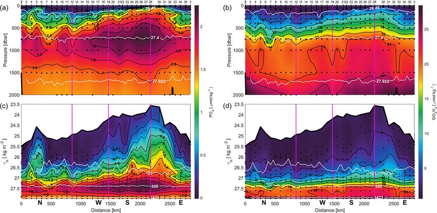
770                                                                N. Burgoa et al.: Cape Verde Frontal Zone in summer 2017

Canary Islands and Cape Blanc, the steady trade winds force          ical processes (Pelegrí and Benazzouz, 2015b). The main
a permanent upwelling (Benazzouz et al., 2014a), which in            biogeochemical processes are related to the availability of
turn triggers an intense southward coastal jet, the Canary           organic matter, O2 and inorganic nutrients in the source re-
Upwelling Current (CUC) (Pelegrí et al., 2005, 2006). Be-            gions and also to remineralization processes; conversely, the
low the CUC and over the continental slope, the Poleward             main physical processes are associated with both the vertical
Undercurrent (PUC) flows northward with remarkable inten-            link between surface and subsurface waters and with the lat-
sity (Barton, 1989; Machín and Pelegrí, 2009; Machín et al.,         eral transports in subsurface waters (Peña-Izquierdo et al.,
2010).                                                               2015; Pelegrí and Benazzouz, 2015b). As a consequence,
   The South Atlantic Central Water (SACW) is the main wa-           the O2 and inorganic nutrient concentrations may vary de-
ter mass on the southern side of the CVFZ. The SACW is               pending on the interplay between the local rate of organic
formed in the subtropical South Atlantic, and it largely mod-        matter remineralization and the rate of water supply (Pelegrí
ifies its thermohaline features along its complex path north-        and Benazzouz, 2015b). In other words, the different dynam-
ward to the CVB (Peña-Izquierdo et al., 2015). The northern          ics between subtropical and tropical regions separated by the
branch of the North Equatorial Countercurrent becomes the            CVFZ, and between oceanic and upwelling regions separated
Cape Verde Current (CVC) at the African slope, carrying the          by the CUF, establish distinct biogeochemical domains with
SACW (Peña-Izquierdo et al., 2015; Pelegrí et al., 2017). The        substantial differences in their O2 and inorganic nutrient pat-
CVC flows anticlockwise around the Guinea Dome (GD)                  terns at the CVB. Over the last 2 decades, several authors
to the southern part of the CVFZ (Peña-Izquierdo et al.,             have focused on the O2 and inorganic nutrient distribution,
2015; Pelegrí et al., 2017). A seasonal pattern has been doc-        considering both the physical properties of water masses and
umented, whereby the GD intensifies in summer as a result            the dynamical processes involved at varying scales (Pelegrí
of the northward penetration of the Intertropical Converge           et al., 2006; Machín et al., 2006; Pastor et al., 2008; Álvarez
Zone (ITCZ) (Siedler et al., 1992; Castellanos et al., 2015).        and Álvarez-Salgado, 2009; Peña-Izquierdo et al., 2012; Pas-
In addition, the northward flow along the African coast also         tor et al., 2013; Peña-Izquierdo et al., 2015; Hosegood et al.,
intensifies in summer due to the relaxation of the trade winds       2017; Burgoa et al., 2020).
south of Cape Blanc, so the Mauritanian Current (MC) and                Here, we address the circulation patterns and the physical
the PUC increase their northward progression to just south of        processes behind the distribution of O2 and inorganic nutri-
Cape Blanc (Siedler et al., 1992; Lázaro et al., 2005).              ents at the dynamically complex CVFZ. To achieve this goal,
   The meeting of southward-flowing CC/CUC with                      we used field observations obtained during the FLUXES-I
northward-flowing PUC/MC leads to a confluence at the                cruise and applied an inverse model to estimate the mass
CVFZ, which fosters the offshore export of mass and seawa-           transports. Additional methods are applied to assess the wa-
ter properties, with its maximum strength in summer (Pastor          ter masses’ distribution both horizontally and with depth (to
et al., 2008). Subtropical and tropical waters exported along        extend the classical definition of the CVF) in order to consis-
the CVFZ exhibit distinct physical–chemical properties.              tently separate the tropical and subtropical sides.
The ENACW is a relatively young, salty and warm water
mass with low nutrient and high oxygen concentrations.
The SACW is an older water mass that is fresher and colder           2     Data and methodology
than the ENACW, and it is largely modified while traveling
through tropical regions; hence, the SACW at the CVFZ is a           2.1    The oceanographic cruise
nutrient-rich and oxygen-poor water mass (Tomczak, 1981;
Zenk et al., 1991; Pastor et al., 2008; Martínez-Marrero             The FLUXES (Carbon Fluxes in a Coastal Upwelling Sys-
et al., 2008; Pastor et al., 2012; Peña-Izquierdo et al., 2015).     tem – Cape Blanc, NW Africa) project included two cruises
The CVF drives nutrient-rich SACW into the southeastern              during 2017 labeled as FLUXES-I and FLUXES-II. The
edge of the nutrient-poor NASG – a process that boosts an            FLUXES-I cruise provided the dataset to conduct the ana-
area of high primary productivity offshore, as revealed by           lyzes presented in this paper. It was carried out from 14 July
the giant filament at Cape Blanc (Gabric et al., 1993; Pastor        to 8 August 2017 aboard the R/V Sarmiento de Gamboa. A
et al., 2013).                                                       grid of 35 stations was selected to form a closed box (pink
   Intermediate levels (∼ 700–1500 m depth) are essentially          dots, Fig. 1). At each station, we sampled the water col-
occupied by modified Antarctic Intermediate Water (AAIW),            umn with a SBE 38 rosette sampler equipped with 24 Niskin
a relatively fresh and cold water mass with high inorganic           bottles of 12 L volume. Temperature, conductivity and oxy-
nutrient and low O2 concentrations. At this latitude, AAIW           gen were measured with a vertical resolution of 1 dbar down
flows northward at 700–1100 m depth along the eastern mar-           to at least 2000 m by means of a CTD SBE 911+. The
gin of both the NASG and NATG (Machín et al., 2006;                  average distance between neighboring CTD (conductivity–
Machín and Pelegrí, 2009; Machín et al., 2010).                      temperature–depth) stations was about 84 km. Shallow sta-
   The distribution of O2 and inorganic nutrients below the          tions 1 and 29 were discarded from the analysis. The sample
euphotic layer is determined by biogeochemical and phys-             grid was split into four transects: the northern transect (N)

Ocean Sci., 17, 769–788, 2021                                                            https://doi.org/10.5194/os-17-769-2021
N. Burgoa et al.: Cape Verde Frontal Zone in summer 2017                                                                           771

                                                                        2.2   Supplementary datasets

                                                                        The Ekman transport through the boundaries of the domain
                                                                        was estimated with daily global wind field observations pro-
                                                                        duced with the Advanced SCATterometer (ASCAT) installed
                                                                        on the EUMETSAT MetOp satellite. This dataset presents a
                                                                        spatial resolution of 0.25 ◦ (Bentamy and Fillon, 2012) and
                                                                        is made available by CERSAT (ftp://ftp.ifremer.fr/ifremer/
                                                                        cersat/products/gridded/MWF/L3/ASCAT/Daily/, last ac-
                                                                        cess: 2 September 2017). Freshwater flux was calculated
                                                                        from the average rates of evaporation and precipitation ex-
                                                                        tracted from the Weather Research and Forecasting model
                                                                        (WRF; Powers et al., 2017) and is provided with a spatial
                                                                        resolution of 0.125 ◦ and a temporal resolution of 12 h.
                                                                           The climatological mean depths of the Neutral Density
                                                                        field during the summer season were evaluated from the cli-
                                                                        matological temperature and salinity fields extracted from
                                                                        the World Ocean Atlas 2018 (WOA18; Locarnini et al., 2018;
                                                                        Zweng et al., 2018). WOA18 was also used to produce a cli-
Figure 1. CTD rosette sampling stations (pink dots) and XBT sam-        matological Neutral Density field during the summer season
ple locations (blue dots) during the FLUXES-I cruise. WOA sta-          to estimate a climatological geostrophic velocity field. Sum-
tions are represented by green dots. Time-averaged wind stress dur-     mer WOA18 nodes were used to extend the N and S tran-
ing the cruise is also represented, with the inset arrow denoting the   sects up to the African coast (green dots, Fig. 1). Finally, two
scale (shown with half of the original spatial resolution).             WOA stations were selected to apply the methodology devel-
                                                                        oped in this paper in order to unveil the vertical location of
                                                                        the CVF (see Sect. 2.4, Fig. 2).
spanned zonally from station 2 to 12 at 23◦ N; the western                 The SEALEVEL_GLO_PHY_L4_REP_OBSERVATIONS
transect (W) was located at 26◦ W from station 12 to 19; the            _008_047 product issued by the Copernicus Ma-
southern transect (S) at 17.5◦ N extended from station 19 to            rine Environment Monitoring Service (CMEMS;
28; the eastern transect (E) closed the box at approximately            http://marine.copernicus.eu, last access: 4 April 2019)
18.6◦ W from station 28 to 3.                                           provided the Level 4 Sea Surface Height (SSH) and derived
   A second observational dataset consisted of 39 expendable            variables as surface geostrophic currents, measured by
bathythermograph probes (XBT-T5, Lockheed Martin Sippi-                 multi-satellite altimetry observations over the global ocean
can, USA) deployed between most CTD stations (blue dots,                with a spatial resolution of 0.25 ◦ . These data captured
Fig. 1). WinMK21 acquisition software was set up to sam-                the mesoscale structures and were helpful to validate the
ple down to 2000 m – a sampling aided by a reduced boat                 near-surface geostrophic field produced by the inversion.
speed during XBT deployment (5 kn). Some XBTs (12, 19,                     GLORYS         12V1      (GLOBAL_REANALYSIS_PHY
30, 31, 38, 39 and 40) were discarded due to malfunction                _001_030) outputs from 25 years, also issued by CMEMS,
during recording.                                                       were used to estimate a summer climatology for the velocity
   Practical salinity (SP ; UNESCO, 1985) was calibrated af-            field, temperature and salinity, with a horizontal resolution of
ter analyzing 51 water samples with a Portasal model 8410A              1/12 ◦ at 50 standard depths. Specifically, the climatological
salinometer, attaining an accuracy and precision within the             salinity was used to present the CVF spatial distribution
values recommended by the World Ocean Circulation Exper-                within the domain (see Sect. 3.2, Fig. 10a).
iment (WOCE). An oxygen sensor SBE 43 was interfaced                       Data treatments (in situ, operational and modeling), in-
with the CTD system during the cruise, and these observa-               terpolations with Data-Interpolating Variational Analysis
tions were later calibrated with 417 in situ samples, provid-           (DIVA, Troupin et al., 2012), graphical representations,
ing a final precision of ± 0.53 µmol kg−1 .                             and the inverse model were coded in MATLAB (MAT-
   Regarding dissolved inorganic nutrients (nitrates, NO3 ;             LAB, 2019). Finally, the Smith–Sandwell bathymetry V19.1
phosphates, PO4 ; and silicates, SiO4 H4 ), 419 water samples           (Smith and Sandwell, 1997) was used in all maps and full-
were collected in Niskin bottles and transferred to 25 mL               depth vertical sections.
polyethylene bottles. These samples were frozen at −20 ◦ C
before their analysis using a segmented flow Alliance Fu-               2.3   Merged hydrographic dataset
tura analyzer following the colorimetric methods proposed
by Grasshoff et al. (1999).                                             A high-resolution in situ temperature field (T ) was produced
                                                                        after merging the CTD and XBT profiles. The remaining

https://doi.org/10.5194/os-17-769-2021                                                                Ocean Sci., 17, 769–788, 2021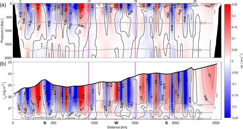
772                                                                   N. Burgoa et al.: Cape Verde Frontal Zone in summer 2017

Figure 2. (a) Map showing the two selected WOA stations in the ENACW (red) and SACW (blue) domains. (b) T –S diagram with the
average salinity for each depth (in the range from 100 to 650 m) shown using black dots between the profiles of the northern and southern
WOA stations. Observations at the same depths are connected by a straight line. (c) Linear, quadratic and cubic fits for depth versus salinity
with the quadratic fit equation.

variables were interpolated to this same new high-resolution             2.4    Tracking the Cape Verde Front
grid to perform additional data treatments.
   SP , O2 , NO3 , PO4 and SiO4 H4 were optimally interpolated           One of the main goals of our study was to estimate the lateral
with DIVA at each transect independently. Before carrying                fluxes on the tropical and subtropical sides of the Cape Verde
out these interpolations, DIVA was applied to the T sup-                 Front. For this, we first had to uncover the location of the
pressing one XBT profile from each transect to validate the              front – both with respect to depth and along its spatial dis-
method. In fact, the interpolated values had a relative error            tribution – within the domain. The classical definition places
< 3.5 % in 75 % of cases. This allows one to set the signal-             the CVF where isohaline 36 meets the 150 m isobath. Here,
to-noise ratio (λ) and the horizontal and vertical correlation           we have developed a method to extend this definition ver-
lengths (Lx and Ly ). Hence, the interpolations of the remain-           tically as follows: two climatological profiles from WOA18
ing hydrological and biogeochemical variables were carried               representative of the ENACW and SACW consistent with the
out with the following parameters: λ = 4, Lx = 110–135 km                definitions given by Tomczak (1981) were selected (Fig. 2a).
and Ly = 50 m. Despite the fact that each variable behaves               Those selected climatological profiles provide an average re-
differently depending on its physical, chemical or biological            lationship between SP , θ and depth, which reveals that the
nature, the correlation scales were considered the same due              traditional definition of the front is based on a salinity value
to the limitation of the sampling resolution. DIVA provided              (36) that indeed corresponds to equal contributions (50 %)
error maps for the gridded fields of each variable which al-             of the ENACW and SACW at 150 m depth. Following the
lowed us to check their accuracy and spatial distribution. A             same reasoning of equal contributions, we calculated the cli-
total of 75 % of the interpolated values of SP and O2 had a rel-         matological salinity that would define the front location at
ative error ≤ 3.5 %. Due to the lower sampling resolution of             standard depths from 100 to 650 m (Fig. 2b).
NO3 , PO4 and SiO4 H4 , their interpolated values had higher                Finally, three linear, quadratic and cubic relationships be-
errors. Between 70 % and 75 % of the interpolated values had             tween salinity and depth were used to infer the salinity that
a relative error ≤ 5.7 %.                                                would define the front location at any given depth. The
   Once the interpolations were performed, Absolute Salinity             quadratic relationship was finally chosen due to its tight fit
(SA ; McDougall et al., 2012) and potential and conservative             to observations (R 2 = 0.998) keeping the polynomial order
temperatures (θ and 2, respectively; McDougall and Barker,               as low as possible (Fig. 2c). Thus, the front location could
2011) were calculated (IOC et al., 2010). In addition, Neutral           be uncovered at the depths occupied by the three layers of
Density (γn ; Jackett and McDougall, 1997) was used as the               central waters (CW).
density variable.

Ocean Sci., 17, 769–788, 2021                                                                   https://doi.org/10.5194/os-17-769-2021
N. Burgoa et al.: Cape Verde Frontal Zone in summer 2017                                                                       773

2.5   Water masses’ distribution                                    ports and the freshwater flux. The reference-level velocity
                                                                    field was then used to estimate the absolute water mass trans-
An optimum multiparameter method (OMP; Karstensen and               port through each transect of the cruise (Martel and Wunsch,
Tomczak, 1998) was used to quantify the contribution to             1993; Paillet and Mercier, 1997; Ganachaud, 2003a; Machín
the observations of the following water types: upper and            et al., 2006; Pérez-Hernández et al., 2013; Hernández-Guerra
lower North Atlantic Deep Water (UNADW and LNADW,                   et al., 2017; Fu et al., 2018; Burgoa et al., 2020).
respectively), Labrador Sea Water (LSW), Mediterranean                 The cruise was carried out over 25 d – a time lag large
Water (MW), AAIW, Subpolar Mode Water (SPMW),                       enough for the structures to evolve during the sampling. This
SACW at 12 ◦ C and 18 ◦ C (SACW12 and SACW18),                      time lag is not generally an issue that would introduce a rel-
ENACW at 12 and 15 ◦ C (ENACW12 and ENACW15),                       evant bias in the calculations; however, in this case, we have
and Madeira Mode Water (MMW). The hydrographic                      a closed volume composed of four hydrographical legs, so
variables used for the analysis were θ , SP , SiO4 H4 , and NO      trying to connect the eastern section with the northern one
(NO = O2 +RN ·NO−     3 , where RN = 1.4 is the stoichiometric      might introduce a large bias in the observations and, con-
ratio of organic matter remineralization; Anderson and              sequently, in the geostrophic velocity field. Hence, to avoid
Sarmiento, 1994; Broecker, 1974). The reference values of           any imbalances induced by the temporal evolution of the sys-
these variables in the source region of each water type were        tem, the volume is closed with land instead of with the east-
extracted from the literature (Pérez et al., 2001; Álvarez          ern transect. To do so, WOA18 climatological nodes were
and Álvarez-Salgado, 2009; Lønborg and Álvarez-Salgado,             used to extend the N and S transects eastward (green dots
2014) and WOA13 (Locarnini et al., 2013; Zweng et al.,              in Fig. 1), where the climatological summer mean of GLO-
2013; Garcia et al., 2014a, b). A linear system of normalized       RYS was also included at the reference level. Therefore, the
and weighted equations for θ , SP , SiO4 H4 , NO and mass           geostrophic velocities at the reference level were modified
conservation was solved to obtain the water type proportions        with the inversion in the N, W and S transects, whereas those
in the observations. Considering the measurement error,             velocities kept their initial climatological summer mean val-
the relative conservative nature and the variability in each        ues from GLORYS in transect E.
variable, the weights assigned to the balance of SiO4 H4 , NO,         The model was made up of eight layers bounded by the
θ and SP were 1, 2, 10 and 10, respectively. A weight of 100        free surface and eight isoneutrals (26.46, 26.85, 27.162,
was imposed on the mass conservation equation assuming              27.40, 27.62, 27.82, 27.922 and 27.962 kg m−3 ), reproduced
the mass was fully conserved. On the other hand, in order           essentially from those defined by Ganachaud (2003a) for the
to solve this undetermined system of equations, the water           North Atlantic Ocean (Fig. 3). The inverse model consid-
types were grouped in a maximum of four according to                ered mass conservation and salinity anomaly conservation
oceanographic criteria. In this way, the unknowns were re-          per layer and also over the whole water column (Ganachaud,
duced from 11 to 5 with the following groups of water types:        2003b). Heat anomaly was introduced only in the deepest
(1) MW–LSW–UNADW–LNADW, (2) SPMW–AAIW–                              layer where it was also considered conservative. Salinity and
MW–LSW, (3) SACW12–ENACW12–SPMW–AAIW,                               heat were added as anomalies to improve the conditioning of
(4) SACW18–ENACW15–SACW12–ENACW12 and (5)                           the model and reduce the linear dependency between equa-
MMW–SACW18–ENACW15. Surface waters (< 100 dbar)                     tions (Ganachaud, 2003b). Therefore, the inverse model was
were excluded from the analysis due to their nonconservative        composed of 19 equations (9 for mass conservation, 9 for
behavior. This OMP with high determination coefficients             salt anomaly conservation and 1 for heat anomaly conserva-
(R 2 > 0.97) and low standard errors of the residuals of θ , SP ,   tion). Those equations were solved using a Gauss–Markov
SiO4 H4 and NO realistically reproduced the thermohaline            estimator for 69 unknowns, comprised of 65 reference-level
and chemical fields during FLUXES-I (Valiente et al., 2021).        velocity adjustments, 3 unknowns for the Ekman transport
                                                                    adjustments (one per transect) and 1 unknown for the fresh-
2.6   Inverse model setup                                           water flux.
                                                                       It was necessary to provide the uncertainties related to the
The lateral geostrophic velocities were calculated at the           noise of the equations (Rnn ) and the unknowns (Rxx ) a pri-
boundaries of the volume closed by hydrographic stations.           ori in order to solve this undetermined system. Rnn and Rxx
Geostrophic velocities were referenced to γn = 27.82 kg m−3         values are compiled in Table 1. The noise of each equa-
(∼ 1333 m, Fig. 3). As an initial guess, the velocities at the      tion depends on the layer thickness, the density field and
reference level were those estimated from the climatological        the variability in the velocity field (Ganachaud, 1999, 2003b;
summer mean provided by GLORYS.                                     Machín et al., 2006). Thus, an analysis of the velocity vari-
   An inverse box model (Wunsch, 1978) was then applied             ability was performed in the mean depths of the eight lay-
to estimate a set of unknowns based on the assumption of            ers. The velocity variance at each layer was estimated from
mass, salt and heat conservation within a closed volume.            summer months in the 25 years of GLORYS data. These
The unknowns in the system are an adjustment of the ini-            variances were transformed into transport uncertainty val-
tial reference-level velocities, an adjustment of Ekman trans-      ues by multiplying by density and the vertical area of the

https://doi.org/10.5194/os-17-769-2021                                                            Ocean Sci., 17, 769–788, 2021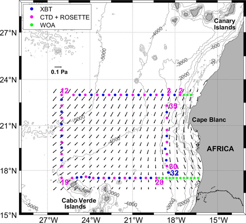
774 N. Burgoa et al.: Cape Verde Frontal Zone in summer 2017
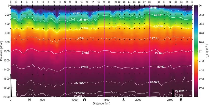
Figure 3. γn vertical section during the FLUXES-I cruise produced with the CTD–XBT merged dataset. White dashed isoneutrals limit the
different water type layers. The direction chosen for the representation of the transects is the course of the vessel. Distance is calculated with
respect to the first station (2). The section is divided as follows: transect N from east to west (from station 2 to 12), transect W from north
to south (from station 12 to 19), transect S from west to east (from station 19 to 28) and transect E from south to north (from station 28 to
3). The northwestern, southwestern and southeastern corners are indicated by three vertical pink lines at stations 12, 19 and 28, respectively.
The sampling points of dissolved oxygen and inorganic nutrients used in this work are represented by black dots.
section involved (Rnn in Table 1). The uncertainty assigned Table 1. A priori noise of equations corresponding to the surface
to the total mass conservation equation was the sum of the water (SW), central water (CW), intermediate water (IW) and deep
uncertainties from the eight mass conservation equations. water (DW) levels and uncertainties of all unknowns of the inverse
The equations for salt and heat anomaly conservation de- model.
pend on the uncertainty of the mass transport, on the variance
of these properties and, specifically, on the layer considered Water levels Rnn [Sv2 ]
(Ganachaud, 1999; Machín, 2003). Therefore, the uncer- SW and CW [2.13–3.3]2
tainties for salt and heat anomaly equations were estimated IW [2.88–3.49]2
as follows (Ganachaud, 1999; Machín, 2003): Rnn (Cq) = DW [1.70]2
a ×var(Cq )×Rnn (mass(q)), where Rnn (Cq) was the uncer-
Unknowns Rxx
tainty in the anomaly equation of the property (salt or heat
anomaly); var(Cq ) was the variance of this property; a was Velocities [10−4 –10−3 ]2 [ms−1 ]2
a weighting factor (4 in the heat anomaly, 1000 in the salt Ekman transports [10−5 –10−4 ]2 [Sv2 ]
anomaly and 106 in the total salt anomaly); q was a given Freshwater flux 0.0042 [Sv2 ]
equation corresponding to a given layer. These variability es-
timates were then included in the inverse model as the a priori
uncertainty of the noise of equations in terms of variances of
variability in the wind stress. An uncertainty of 50 % of the
mass, salt anomaly and heat anomaly transports.
initial value of the freshwater flux, which was 0.0935 Sv, was
The variance of the velocities in the reference level was
also considered (Ganachaud, 1999; Hernández-Guerra et al.,
used as a measure of the a priori uncertainty for these un-
2005; Machín et al., 2006). The Ekman transports, the fresh-
knowns. These variances were also calculated from the sum-
water flux and their uncertainties (Rxx in Table 1) were added
mer months’ velocities provided by GLORYS (Rxx in Ta-
to the inverse model in the shallowest layer for mass and salt
ble 1).
anomaly as well as in the total mass transport and total salt
The initial Ekman transports were estimated from the av-
anomaly transport equations.
erage wind stress during the days of the cruise. A 50 % un-
Dianeutral transfers between layers were considered to be
certainty was assigned to the initial estimate of Ekman trans-
negligible compared with other sources of lateral transports,
ports, related to the errors in their measurements and to the
so they were not included in the inversion. Furthermore, the
Ocean Sci., 17, 769–788, 2021 https://doi.org/10.5194/os-17-769-2021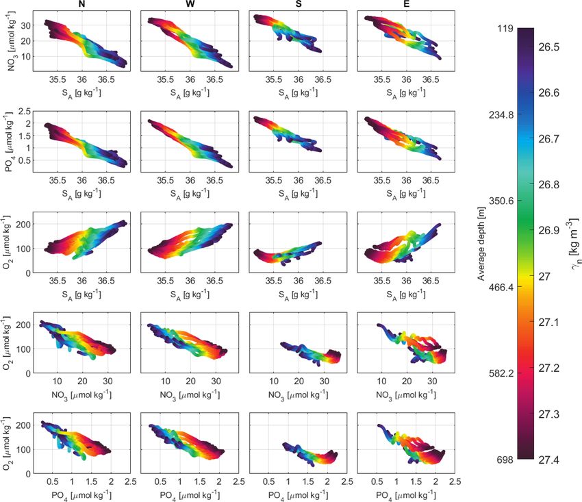
N. Burgoa et al.: Cape Verde Frontal Zone in summer 2017 775
inverse model only works with information from the box In IW, the O2 distribution was quite uniform in all tran-
boundaries and cannot be used to provide any spatial details sects, presenting a slight increase with depth. With respect to
of dianeutral fluxes for a given interface between layers, just inorganic nutrients, their concentrations in transect N were
an average value for the whole interface (Burgoa et al., 2020). lower than in the remaining transects, which were occupied
The resulting absolute geostrophic velocity field allowed by a larger amount of AAIW. Indeed, the largest NO3 and
us to calculate transports of O2 and inorganic nutrients. PO4 concentrations were registered as being associated with
Those transports were obtained by multiplying their con- AAIW at around 1000 m in transects S and E (Figs. 6, 7).
centration by mass transports, so their concentrations were Finally, in the deepest layer, high concentrations of O2 and
initially interpolated to the positions where the absolute inorganic nutrients were found. Specifically, the highest con-
geostrophic velocities were estimated. centrations of SiO4 H4 were recorded in this deepest layer.
The hydrological and biogeochemical characteristic of the
water masses are summarized in Figs. 8 and 9, where the re-
3 Results lationships between in situ measurements of SA , O2 , NO3
and PO4 are displayed. These property–property distribu-
3.1 Hydrography and water masses
tions might be used to define the characteristic values of the
The main water masses sampled during FLUXES-I were the water masses in the domain (Emery, 2001). In CW, inverse
ENACW (merging the MMW, ENACW15 and ENACW12) tight relationships are obtained for NO3 and PO4 with SA ,
and the SACW (SACW18 and SACW12) below the mixing whereas the relationship is direct and looser for O2 with SA .
layer and above 700 m; the modified AAIW and MW from In IW, the relationships between NO3 and PO4 with SA are
700 up to 1700 m; and the North Atlantic Deep Water (the much less defined, with an “S”-like pattern. In all cases, the
LSW and UNADW) below 1600 m (Figs. 3, 4, 5; Zenk et al., relationships between O2 and NO3 or O2 and PO4 are rather
1991; Martínez-Marrero et al., 2008; Pastor et al., 2012). tight and inverse.
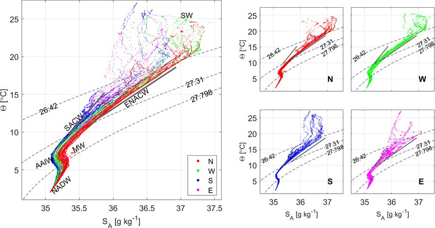
2−SA definitions proposed by Tomczak (1981) for the salty The previous distributions are presented from a large-scale
and warm ENACW and the fresh and cold SACW (straight perspective. A second reading of the dataset might be per-
lines in Fig. 4) were used to identify CW in all transects: formed, emphasizing the role played by mesoscale struc-
the main water mass sampled in transects N and W was the tures. For instance, an intrathermocline anticyclonic eddy
ENACW (∼ 36.15 g kg−1 at 300 m), whereas the SACW was centered in station 4 was detected in 2, SA , O2 , NO3 and
dominant in transect S (∼ 35.65 g kg−1 at 300 m). Both the PO4 (Figs. 5, 6, 7). On the other side, the CVF was also de-
ENACW and SACW were registered along transect E. Wa- tected in transects S and E as a sharp transition in all proper-
ter masses were also well defined at intermediate levels, with ties (Figs. 5, 6, 7). In particular, O2 presented two remarkable
colder and fresher AAIW over warmer and saltier MW. MW minimum values of 60 µmol kg−1 between 100 and 150 m
was sampled mainly in transect N and in smaller proportions when the frontal area was crossed (Fig. 6). Just below these
in the northern part of transects E and W, whereas the AAIW O2 minima, the local maxima of NO3 , PO4 and SiO4 H4 were
was the main water mass recorded in transects S, E and W recorded (Figs. 6, 7).
(Fig. 4).
Figure 3 presents the high-resolution γn field once the 3.2 Cape Verde Front
XBTs were considered. The upper four layers transported
surface waters (SW, first layer above 26.46 kg m−3 ) and The CVF has historically been defined at only one depth,
CW (between 26.46 and 27.40 kg m−3 ); intermediate wa- where isohaline 36 (or 36.15 g kg−1 , Burgoa et al., 2020) in-
ters (IW) flowed along the next three layers between 27.40 tersects isobath 150 m (Zenk et al., 1991). Following that def-
and 27.922 kg m−3 , whereas deep waters (DW) flowed in the inition, the CVF could be located during FLUXES-I between
deepest layer below 27.922 kg m−3 . stations 23 and 24 in transect S, where 1SA > 0.70 g kg−1
The overall distributions of O2 , NO3 , PO4 and SiO4 H4 at and 12 > 1.92 ◦ C were observed between both sides of the
CW were highly variable and closely related to the location front; CVF was also detected between stations 33 and 34 in
of the different water masses. In transects N and W, where transect E with lower 1SA > 0.30 g kg−1 and 12 > 1.10 ◦ C
ENACW was dominant, the O2 concentrations were higher values (Fig. 5).
than in transects S and E where SACW was found, with min- The method developed in this paper to estimate the ver-
imum O2 values lower than 60 µmol kg−1 at 300 m (Fig. 6). tical location of the front depicted a complex spatial distri-
In contrast, the concentrations of the three inorganic nutri- bution (Fig. 10). The CVF is represented by several isoha-
ents in these last two transects were higher than in transects lines associated with specific depths. These isohalines un-
N and W at CW levels, with concentrations of around 27– veil that the front was almost completely vertical in tran-
30 µmol kg−1 for NO3 , 1.5–1.7 µmol kg−1 for PO4 and 7.5– sect E, while in the southwestern corner it presented a no-
9.9 µmol kg−1 for SiO4 H4 at 300 m depth (Figs. 6, 7). table slope with its surface end located south of its deep end.
Hence, the front was oriented from northeast to southwest
at near-surface layers, whereas it presented a roughly east–
https://doi.org/10.5194/os-17-769-2021 Ocean Sci., 17, 769–788, 2021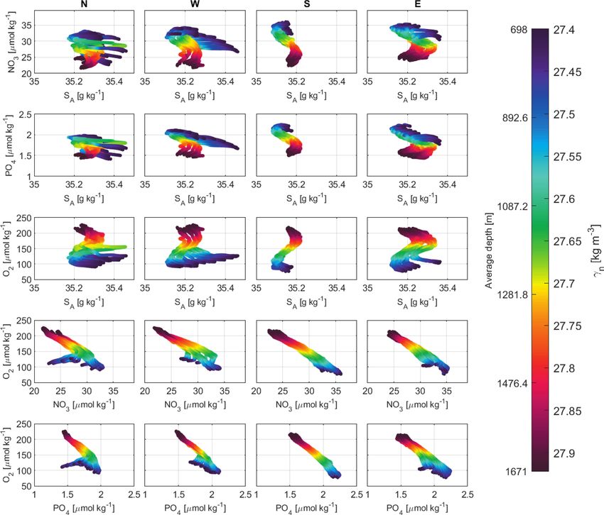
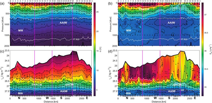
776                                                                    N. Burgoa et al.: Cape Verde Frontal Zone in summer 2017

Figure 4. 2 − SA diagrams during the FLUXES-I cruise. The different water masses in the northern (N, red dots), western (W, green
dots), southern (S, blue dots) and eastern (E, pink dots) transects for surface waters (SW), North Atlantic Central Water (ENACW), South
Atlantic Central Water (SACW), modified Antarctic Intermediate Water (AAIW), Mediterranean Water (MW) and North Atlantic Deep
Water (NADW). Potential density anomaly contours (gray dashed lines) equivalent to 26.46, 27.4 and 27.922 kg m−3 isoneutrals delimit the
surface, central, intermediate and deep water levels. Straight lines represent the 2 − SA relationship for ENACW and SACW equivalent to
that proposed by Tomczak (1981).

Figure 5. Sections of 2 (a, c) and SA (b, d) with respect to depth (upper line) and γn (lower line) during the FLUXES-I cruise. The direction
chosen for the representation is the same as in Fig. 3. The northwestern, southwestern and southeastern corners are indicated by three vertical
pink lines at stations 12, 19 and 28, respectively. In depth sections, the isoneutrals that delimit the surface, central, intermediate and deep
water are represented by white contours. In γn sections, the depths of 150, 698 and 1671 m are also shown. The sampling points for dissolved
oxygen and inorganic nutrients used in this work are represented by black dots. Sections are only estimated with the CTD–XBT merged
dataset.

Ocean Sci., 17, 769–788, 2021                                                                   https://doi.org/10.5194/os-17-769-2021
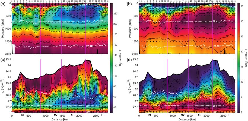
N. Burgoa et al.: Cape Verde Frontal Zone in summer 2017                                                                                        777

Figure 6. Sections of O2 (a, c) and NO3 (b, d) with respect to depth (upper line) and γn (lower line) during the FLUXES-I cruise. The
direction chosen for the representation is the same as in Fig. 3. The northwestern, southwestern and southeastern corners are indicated by
three vertical pink lines at stations 12, 19 and 28, respectively. In depth sections, the isoneutrals that delimit the surface, central, intermediate
and deep water are represented by white contours. In γn sections, the depths of 150, 698 and 1671 m are also shown. The sampling points of
O2 and NO3 used in this work are represented by black dots.

Figure 7. Sections of PO4 (a, c) and SiO4 H4 (b, d) with respect to depth (upper line) and γn (lower line) during the FLUXES-I cruise. The
direction chosen for the representation is the same as in Fig. 3. The northwestern, southwestern and southeastern corners are indicated by three
vertical pink lines at stations 12, 19 and 28, respectively. In depth sections, the isoneutrals which delimit the surface, central, intermediate
and deep water are represented by white contours. In γn sections, the depths of 150, 698 and 1671 m are also shown. The sampling points of
PO4 and SiO4 H4 used in this work are represented by black dots.

https://doi.org/10.5194/os-17-769-2021                                                                          Ocean Sci., 17, 769–788, 2021
778 N. Burgoa et al.: Cape Verde Frontal Zone in summer 2017
Figure 8. Scatterplots of in situ observations of NO3 (first row), PO4 (second row) and O2 (third row) (in µmol kg−1 ) with respect to SA and
γn (in color with an approximate scale of the average depths) in the north (N, first column), west (W, second column), south (S, third column)
and east (E, fourth column) transects for CW layers. In the fourth and fifth rows, scatterplots of NO3 –O2 and PO4 –O2 in four transects for
the CW layers are shown.
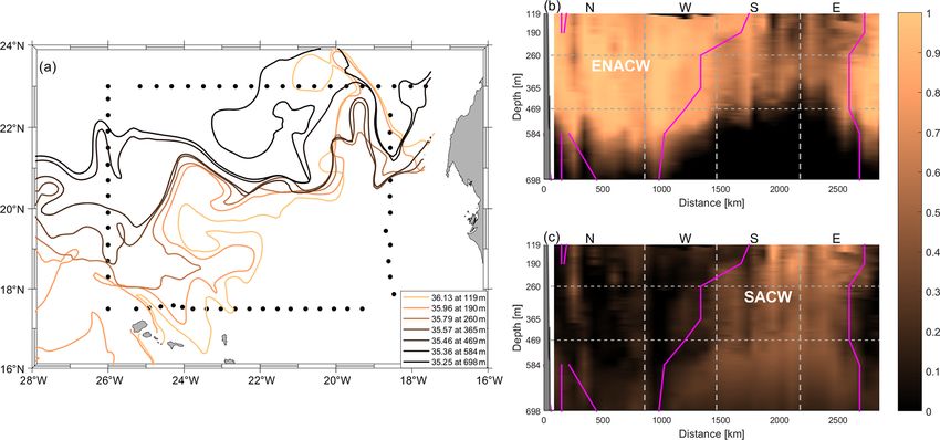
west orientation at 698 m depth (Fig. 10a). On the other hand, mainly associated with the first and third layers (black line in
the CVF location presented with this methodology is indi- Fig. 11b), likely related to mesoscale structures undersam-
cated along the transects (pink lines), revealing a remarkable pled during the cruise.
match with the distributions of the maximum contributions Large transports are obtained in the entire water column.
of ENACW (MMW–ENACW15–ENACW12) and SACW In the two shallowest layers, the mass exchange is basically
(SACW18–SACW12) estimated with the OMP (Fig. 10b, c). from north and south to the west, carrying some 3.4 Sv. In the
third and fourth layers, transports continued entering from
3.3 Inverse model solution the south, whereas transports reversed in the N and W tran-
sects, flowing a total of some 1 Sv. At IW levels, the esti-
The inverse model provided absolute geostrophic veloci- mated transports were moderately high and northward, with
ties for transects N, W and S, extended to the coast with more than 3 Sv that entered through the W and S transects. At
WOA nodes. Mass transports were then evaluated to esti- DW levels, the integrated mass transports were around 1 Sv,
mate the mass imbalance within the closed box. Figure 11 maintaining the IW levels’ scheme.
presents the mass transports accumulated along transects N, The results obtained from the inversion are compared with
W and S, grouped by different water levels (panel a); the fig- two independent databases: transports from altimetry and
ure also shows the transports integrated per layer and tran- transports from the GLORYS numerical model (Fig. 12).
sect (panel b). Note that positive (negative) values repre- These transports are calculated by multiplying the velocity at
sent outward (inward) transports from (to) the closed box the surface by the vertical area covered by the first layer in the
(1 Sv = 109 kg s−1 ). The mass transport imbalance in ev- inverse model. Accordingly, in the case of the inverse model
ery water level was roughly zero once it was accumulated we have used the accumulated mass transports in the first
along the box, indicating that the mass was highly conserved layer. The overall transport structure is rather similar for all
(Fig. 11a). An imbalance was observed in the net transport
Ocean Sci., 17, 769–788, 2021 https://doi.org/10.5194/os-17-769-2021N. Burgoa et al.: Cape Verde Frontal Zone in summer 2017 779 Figure 9. Scatterplots of in situ observations of NO3 (first row), PO4 (second row) and O2 (third row) (in µmol kg−1 ) with respect to SA and γn (in color with an approximate scale of the average depths) in the north (N, first column), west (W, second column), south (S, third column) and east (E, fourth column) transects for IW layers. In the fourth and fifth rows, scatterplots of NO3 –O2 and PO4 –O2 in four transects for the IW layers are shown. Figure 10. (a) Location of the front at the 36.07, 35.88, 35.67, 35.43, 35.31, 35.2 and 35.08 isohalines, corresponding to average depths of 119, 190, 260, 365, 469, 584 and 698 m, equivalent to 26.46, 26.63, 26.85, 26.98, 27.162, 27.28 and 27.40 kg m−3 , respectively. Vertical sections of the three layers of CW with the percentages of ENACW (b) and SACW (c), and the front location superimposed by pink lines. The direction chosen for the representation is the same as in Fig. 3. The northwestern, southwestern and southeastern corners are indicated by three vertical gray dashed lines. Three layers are also separated by two horizontal gray dashed lines. https://doi.org/10.5194/os-17-769-2021 Ocean Sci., 17, 769–788, 2021
780                                                                     N. Burgoa et al.: Cape Verde Frontal Zone in summer 2017

                                                                          Figure 12. Accumulated mass transports in the first layer of SW
                                                                          estimated along the N, W and S transects (without WOA stations)
                                                                          with altimetry-derived geostrophy (red line), inversion (with GLO-
                                                                          RYS data as reference velocities, black line) and the GLORYS field
                                                                          (blue line). Negative (positive) values indicate inward (outward)
                                                                          transports, as in Fig. 11. The northwestern and southwestern cor-
                                                                          ners (at stations 12 and 19) are indicated by vertical dashed lines.

                                                                          the largest velocities are mainly found in the upper 200–
                                                                          300 m depth.
                                                                             This velocity field helps to identify several mesoscale fea-
Figure 11. (a) Accumulated mass transports per SW, CW, IW and
                                                                          tures captured during the cruise. Besides the intrathermo-
DW levels, and (b) mass transports integrated per north, west and
                                                                          cline anticyclonic eddy located between stations 3 and 5, an-
south transect, estimated by the inverse model during the FLUXES-
I cruise (including WOA stations in transects N and S). Negative          other cyclonic eddy was centered between stations 5 and 7,
(positive) values indicate inward (outward) transports in both plots.     next to the first eddy. Transect N was also crossed by a sec-
Mass conservation in the whole domain close to the coast is shown         ond anticyclonic eddy between stations 9 and 12. The main
by the black line. The northwestern and southwestern corners are          mesoscale structures sampled in transect W were a meander
indicated by vertical dashed lines at stations 12 and 19 in the ac-       between stations 15 and 18 and an intrusion found between
cumulated mass transports (a). The horizontal bars in each layer          stations 18 and 19, which actually entered the box through
represented by the net mass transport are the errors estimated by the     the southwestern corner. A second part of this intrusion is
inverse model (b).                                                        observed in transect S, where it entered the box between sta-
                                                                          tions 19 and 20 and left between stations 20 and 21. From
                                                                          stations 22 to 26, some additional meandering was observed
three cases, in particular between the inverse model and the              along transect S. A cyclonic eddy had a notable negative ve-
altimetry. GLORYS might not be recovering the mesoscale                   locity in the middle part of transect S centered at station 27.
signal, and its low response to this variability is likely caus-
ing it to deviate from the other two databases. In all cases,             3.5   Inorganic nutrient and O2 transports
the final imbalance is quite similar – about 1.5–2 Sv.
                                                                          The transports (integrated per water level and transect) for
3.4   Geostrophic velocity                                                O2 , NO3 , PO4 and SiO4 H4 are presented in Fig. 14 and com-
                                                                          piled in Table 2. At IW and DW levels, the transports for all
The previous result is now applied to present the geostrophic             properties are nearly balanced and may be described as a net
velocities along the three transects developed to perform                 northward transport with contributions from the western and
the inverse model. Figure 13 displays the absolute velocity               southern transects.
field perpendicular to each transect with a geographic crite-                However, the transports at the SW and CW levels present
ria (positive velocities are northward and eastward). The ab-             an imbalanced distribution that can not be fully related to
solute velocity field might be described as alternating vertical          imbalances in the mass transports, as mass transports are
cells with velocities in the range from −0.25 to 0.25 m s−1 ;             nearly balanced at those water levels. Transports present a

Ocean Sci., 17, 769–788, 2021                                                                   https://doi.org/10.5194/os-17-769-2021
N. Burgoa et al.: Cape Verde Frontal Zone in summer 2017 781
Table 2. Mass transports and their errors (in Sv), and transports of O2 , NO3 , PO4 and SiO4 H4 (in kmol s−1 ) with their errors relative to
mass transport for SW, CW, IW and DW across the northern, western, southern and eastern transects for the FLUXES-I cruise (with WOA
stations). Positive (negative) values indicate outward (inward) transports. The total row of each inorganic nutrient or O2 is its integrated
transport throughout the whole water column. The last column is the maladjustment or imbalance of each water level.
Transport Water level North West South Imbalance
SW −1.80 ± 0.75 2.32 ± 0.79 −0.89 ± 0.59 −0.37 ± 1.24
CW −0.03 ± 1.49 1.44 ± 1.62 −1.49 ± 1.73 −0.08 ± 2.80
CW [Sv] IW 3.43 ± 2.54 −1.52 ± 2.73 −1.87 ± 2.55 0.05 ± 4.52
DW 0.99 ± 0.99 −0.62 ± 1.07 −0.06 ± 1.04 0.31 ± 1.79
Total 2.59 ± 3.19 1.62 ± 3.44 −4.31 ± 3.31 −0.09 ± 5.74
SW −480.79 ± 198.59 379.80 ± 129.89 −40.79 ± 27.09 −141.77 ± 225.46
CW −166.13 ± 764.92 71.14 ± 79.95 −131.51 ± 152.72 −226.49 ± 489.00
O2 [kmol s−1 ] IW 603.63 ± 446.28 −296.60 ± 530.85 −283.33 ± 387.17 23.70 ± 794.27
DW 223.75 ± 222.64 −141.27 ± 244.20 −15.25 ± 263.23 67.23 ± 222.93
Total 180.46 ± 222.42 13.08 ± 27.77 −470.88 ± 361.33 −277.34 ± 975.37
SW −7.39 ± 3.05 22.54 ± 7.71 14.65 ± 9.73 29.80 ± 47.39
CW 32.64 ± 150.30 42.88 ± 48.19 19.22 ± 22.32 94.74 ± 204.5
NO3 [kmol s−1 ] IW 89.91 ± 66.47 −41.65 ± 74.55 −43.90 ± 60.00 4.36 ± 242.61
DW 22.56 ± 22.45 −13.97 ± 24.15 −2.06 ± 35.47 6.53 ± 21.70
Total 137.72 ± 169.74 9.80 ± 20.81 −12.09 ± 9.28 135.43 ± 476.30
SW −0.45 ± 0.18 1.47 ± 0.50 1.01 ± 0.67 2.04 ± 3.24
CW 2.02 ± 9.32 2.59 ± 2.91 1.32 ± 1.53 5.94 ± 12.82
PO4 [kmol s−1 ] IW 5.83 ± 4.31 −2.47 ± 4.42 −2.70 ± 3.69 0.65 ± 36.36
DW 1.45 ± 1.44 −0.91 ± 1.56 −0.08 ± 1.37 0.46 ± 1.53
Total 8.85 ± 10.91 0.69 ± 1.47 −0.45 ± 0.35 9.09 ± 31.96
SW −3.63 ± 1.50 7.30 ± 2.50 4.59 ± 3.05 8.27 ± 13.15
CW 20.68 ± 95.22 16.00 ± 17.98 7.00 ± 8.13 43.68 ± 94.29
SiO4 H4 [kmol s−1 ] IW 74.49 ± 55.07 −33.46 ± 59.88 −34.98 ± 47.80 6.05 ± 336.72
DW 25.70 ± 25.57 −14.76 ± 25.52 −2.26 ± 38.92 8.68 ± 28.71
Total 117.24 ± 144.50 −24.92 ± 52.92 −25.65 ± 19.68 66.67 ± 234.49
distribution where O2 enters the box through transects N by Wanninkhof (2014), using an average wind speed for the
and S; a lower amount of O2 leaves the box through tran- whole domain (U , in m s−1 ) and the Schmidt number (Sc)
sect W, revealing a net O2 decay within the box. The high- for O2 to estimate the gas transfer velocity (k, in cm h−1 ) as
est O2 transports are obtained at the SW levels, as a com- k = 0.251 < U 2 > (Sc/660)−0.5 . We then estimated the av-
bined effect of large velocities and high O2 concentration in erage apparent oxygen utilization (AOU); the O2 transport
the photosynthetic layer in contact with the atmosphere. Fi- from the sea surface to the atmosphere is also estimated as
nally, the pattern in the transports’ distribution is quite the F = −kAOUA/1000, where A is the surface area of the do-
same for NO3 , PO4 and SiO4 H4 : nutrients leave the domain main (m2 ). These calculations provide an O2 export to the
through transects N, W and S, with a tiny amount entering atmosphere of 113.54 kmol s−1 . This number indicates that
the box through transect N at the SW and CW levels. The the total O2 consumption within the box is 163.8 kmol s−1 ,
lowest transports for inorganic nutrients are obtained in the as the lateral transport integrated for the whole sampled wa-
SW layer, as a consequence of nutrient depletion within the ter column was −277.34 kmol s−1 . On the other hand, the
photic layer, whereas the highest transports are observed at inorganic nutrient positive balances indicate that the domain
CW and IW levels. A large imbalance is obtained at CW lev- is producing inorganic nutrients, likely as a consequence of
els, providing a net nutrient increase within the box at CW remineralization below the photic layer; the nutrient import
levels. from the atmosphere is considered negligible compared with
Biogeochemical budgets can be obtained for the entire wa- lateral transports, according to climatological values reported
ter column once we have produced the net lateral transports by Fernández-Castro et al. (2019). Hence, this domain would
of O2 and inorganic nutrients (Table 2). To do so, we first be acting as an heterotrophic box, as revealed by the net oxy-
still need to estimate the O2 exchange between the sea sur- gen consumption, with remineralization of N, P and Si below
face and the atmosphere. We have proceeded as documented the photic layer.
https://doi.org/10.5194/os-17-769-2021 Ocean Sci., 17, 769–788, 2021782 N. Burgoa et al.: Cape Verde Frontal Zone in summer 2017 Figure 13. Sections of the absolute geostrophic velocity perpendicular to each transect with respect to depth (a) and γn (b) during the FLUXES-I cruise (including WOA stations). The velocity sign was selected on geographic criteria (positive sign northward and eastward). The direction chosen for the representation is the same as in Fig. 3. The zero contour line is the thick black line. The northwestern and southwestern corners are indicated by vertical pink lines at stations 12 and 19. In depth sections, the isoneutrals that delimit the surface, central, intermediate and deep water are represented by gray contours. In γn sections, the depths of 150, 698 and 1671 m are also shown. Figure 14. O2 , NO3 , PO4 and SiO4 H4 transports (in kmol s−1 ) integrated per water-type level (SW, CW, IW and DW) in the north (N, pink line), west (W, green line) and south (S, blue line) transects during the FLUXES-I cruise (including WOA stations). The black line represents the net transport of each biochemical variable. See Table 2 to check the O2 , NO3 , PO4 and SiO4 H4 transports’ values in each layer per transect. Negative (positive) values indicate inward (outward) transports, as in Fig. 11. Ocean Sci., 17, 769–788, 2021 https://doi.org/10.5194/os-17-769-2021
N. Burgoa et al.: Cape Verde Frontal Zone in summer 2017                                                                           783

4   Discussion

We have presented the dynamics related to the water masses
and their O2 and inorganic nutrient content in the transition
between the eastern NASG and the NATG during summer
2017. The water masses’ distribution in the CVFZ during
FLUXES-I is consistent with that documented previously
(Hernández-Guerra et al., 2005; Pastor et al., 2012; Peña-
Izquierdo et al., 2012; Burgoa et al., 2020): a latitudinal
change between the ENACW and SACW below the mix-
ing layer and above 700 m was detected from north to south
(Pelegrí et al., 2017), while a second latitudinal transition
was observed in IW between AAIW and MW from south
to north (Zenk et al., 1991), with AAIW being the dominant
water mass. The characteristic of these water masses are con-
ditioned by their origin and the path followed on their way
to the CVB. While transects N and S present well-defined
water masses, transects W and E reflect a water masses tran-
sition between transects N and S. The upwelling filaments
off the coast of Cape Blanc are examples of mesoscale and          Figure 15. Mass (109 kg s−1 ), O2 , NO3 , PO4 and SiO4 H4 trans-
submesoscale structures associated with the frontal systems.       ports (in kmol s−1 ) integrated per water-type level (SW, CW, IW
(Meunier et al., 2012; Lovecchio et al., 2018; Appen et al.,       and DW) through transect E during the FLUXES-I cruise. Eastward
2020). The ENACW and SACW property distributions pre-              transports were defined as positive. The O2 (PO4 ) transport is rep-
sented in Figure 8 compare well with those reported by Pas-        resented as being divided (multiplied) by 10.
tor et al. (2008) and Pelegrí and Benazzouz (2015b). At IW
levels, the variability is mainly related to the AAIW flowing
                                                                   Table 3. Total imbalances of mass, O2 , NO3 , PO4 and SiO4 H4
northward to the Canary Islands basin (Machín and Pelegrí,         transports in the subtropical and tropical areas separated by the CVF
2009; Machín et al., 2010). The shadow zone documented             at the three CW layers. All imbalances are estimated from the inte-
by Kawase and Sarmiento (1985) and the development of              grated transports from each respective side of the front and consid-
an oxygen minimum zone (OMZ) within the CW and IW                  ering transports between WOA stations.
levels was centered in transect S between 100 and 800 m
depth with its core around 400 m between isoneutrals 27.1            Transport                      Subtropical             Tropical
and 27.3 kg m−3 (Karstensen et al., 2008; Brandt et al., 2015;                                       imbalance            imbalance
Thomsen et al., 2019). That distribution matches well with
                                                                     CW [Sv]                      0.56 ± 1.47        −0.63 ± 1.68
the one provided by Peña-Izquierdo et al. (2015), with high
                                                                     O2 [kmol s−1 ]          −153.12 ± 714.98      −73.38 ± 134.08
concentrations of NO3 and PO4 .
                                                                     NO3 [kmol s−1 ]           46.68 ± 133.26        47.07 ± 99.62
   A major contribution from this paper is the development of        PO4 [kmol s−1 ]             2.88 ± 11.36          3.05 ± 6.20
an extended version of the classical methodology applied to          SiO4 H4 [kmol s−1 ]       23.37 ± 109.32        20.32 ± 44.14
locate the CVF. Following the definitions of the SACW and
ENACW reported by Tomczak (1981) and the interpretation
of the CVFZ by Zenk et al. (1991), the front 3-D structure
from 150 to 650 m depth has been produced by combining             the front. The CVF also influenced its adjacent waters, as ob-
in situ and GLORYS data (Fig. 10). Fist of all, we would           served, for example, in the minima of O2 and the maxima of
like to highlight the consistency between the results produced     NO3 and PO4 sampled just below 150 m in the tropical side
from the in situ observations compared to the results from the     of the front, which might be indicating a local remineraliza-
GLORYS model. The front spatial disposition reveals that           tion (Fig. 6) (Thomsen et al., 2019).
the CVF is a complex meandering front with several associ-            The main limitations in the present analyzes were related
ated mesoscale features, showing a variable geographical ori-      to the high relative importance of mesoscale features in the
entation at different depths (Barton, 1987; Martínez-Marrero       domain. These features modify the thermohaline field with
et al., 2008; Pastor et al., 2008, 2012). The vertical distribu-   an intensity capable of inducing transports of approximately
tion of the CVF enables the interpretation of the imbalances       the same order of magnitude as those related to the large-
in lateral transports of mass, O2 and inorganic nutrients at       scale circulation (Volkov et al., 2008; Zhang et al., 2014).
both sides of the front (Table 3). The predominance (lack) of      On the one hand, if the mesoscale field is undersampled, it
SACW (ENACW) in transect S suggests that the CVF may               might induce large imbalances when quantifying the large-
be functioning as a barrier against lateral transports across      scale transports. On the other hand, the important dynam-

https://doi.org/10.5194/os-17-769-2021                                                              Ocean Sci., 17, 769–788, 2021
You can also read