Conditional simulation of spatial rainfall fields using random mixing: a study that implements full control over the stochastic process - HESS
←
→
Page content transcription
If your browser does not render page correctly, please read the page content below
Hydrol. Earth Syst. Sci., 25, 3819–3835, 2021
https://doi.org/10.5194/hess-25-3819-2021
© Author(s) 2021. This work is distributed under
the Creative Commons Attribution 4.0 License.

Conditional simulation of spatial rainfall fields
using random mixing: a study that implements
full control over the stochastic process
Jieru Yan1, , Fei Li1, , András Bárdossy2 , and Tao Tao1
1 Collegeof Environmental Science and Engineering, Tongji University, Shanghai, China
2 Institute
          for Modelling Hydraulic and Environmental Systems, Department of Hydrology and Geohydrology,
University of Stuttgart, Stuttgart, Germany
 These authors contributed equally to this work.

Correspondence: Tao Tao (taotao@tongji.edu.cn)

Received: 29 January 2021 – Discussion started: 2 February 2021
Revised: 10 May 2021 – Accepted: 30 May 2021 – Published: 2 July 2021

Abstract. The accuracy of spatial precipitation estimates            radar–gauge merging techniques: ordinary Kriging, Kriging
with relatively high spatiotemporal resolution is of vital im-       with external drift, and conditional merging, and the sensitiv-
portance in various fields of research and practice. Yet the         ity of the approach to two factors – the number of rain gauges
intricate variability and intermittent nature of precipitation       and the random error in the radar estimates – is analysed in
make it very difficult to obtain accurate spatial precipitation      the same experimental context.
estimates. Radars and rain gauges are two complementary
sources of precipitation information: the former are inaccu-
rate in general but are valid indicators of the spatial pattern
                                                                     1   Introduction
of the rainfall field; the latter are relatively accurate but lack
spatial coverage. Several radar–gauge merging techniques             Precipitation is one of the most important factors in hydrol-
that can provide spatial precipitation estimates have been           ogy and meteorology. The accuracy of spatial precipitation
proposed in the scientific literature. Conditional simulation        estimates with relatively high spatiotemporal resolution is
has great potential to be used in spatial precipitation estima-      of vital importance in various fields of research and prac-
tion. Unlike commonly used interpolation methods, condi-             tice, such as the promotion of meteorological and hydrolog-
tional simulation yields a range of possible estimates due to        ical monitoring, forecasting performed to enhance our abil-
its Monte Carlo framework. However, one obstacle that ham-           ity to cope with natural disasters, the study of climate trends
pers the application of conditional simulation in spatial pre-       and variability, and the management of water resources (Yil-
cipitation estimation is the need to obtain the marginal distri-     maz et al., 2005; Michaelides et al., 2009; Jiang et al., 2012;
bution function of the rainfall field with sufficient accuracy.      Liu et al., 2017). Yet, unlike many other hydrometeorologi-
In this work, we propose a method to obtain the marginal             cal variables such as temperature and humidity, precipitation
distribution function from radar and rain gauge data. A con-         occurs intermittently in space and time, i.e. nonrainy areas
ditional simulation method, random mixing (RM), is used to           occur amidst rainy areas, and dry periods occur amidst wet
simulate rainfall fields. The radar and rain gauge data used         periods (Kumar and Foufoula-Georgiou, 1994). The intricate
in the application of the proposed method are derived from           spatiotemporal variability and intermittent nature of precip-
a stack of synthetic rainfall fields. Due to the full control        itation make it very difficult to obtain accurate spatial pre-
over the stochastic process, the accuracy of the estimates           cipitation estimates (Emmanuel et al., 2012; Cristiano et al.,
is verified comprehensively. The results from the proposed           2017).
approach are compared with those from three well-known

Published by Copernicus Publications on behalf of the European Geosciences Union.
3820                                       J. Yan et al.: Conditional simulation of spatial rainfall fields using random mixing

   Rain gauges – the only devices that directly measure pre-           number, simulation can provide a better solution by yield-
cipitation on the ground surface – are still considered the            ing a range of possible outcomes. In the context of merging
most reliable source of precipitation information in hydrol-           radar and rain gauge data, simulation is often performed un-
ogy. However, rain gauges are only available at limited lo-            der constraints (such as equality constraints at rain gauge lo-
cations. The representativeness of gauge observations for              cations or the field pattern indicated by radar). There are sev-
the entire precipitation field is therefore limited. Significant       eral methods that simulate spatially random fields using cer-
research has shown that precipitation estimation based on              tain covariance functions in Gaussian space, such as turning
gauge observations suffers from degraded levels of accuracy            bands simulation, LU-decomposition-based methods, and se-
during storms with increased rainfall intensities, when con-           quential Gaussian simulation (Mantoglou and Wilson, 1982;
vective processes are significant (Adams, 2016). Meteoro-              Deutsch and Journel, 1998; Chilès and Delfiner, 2000; Lan-
logical radar, on the other hand, is a superb tool for measur-         tuéjoul, 2002). Studies on conditional simulation of rainfall
ing spatial patterns of reflectivity at the altitude of the mea-       fields are, however, rare. One of the major obstacles that
surement. Yet radar-based precipitation estimation can be              hampers the application of conditional simulation in spatial
problematic due to various sources of errors, e.g. variations          precipitation estimation is the need to obtain the marginal
in the vertical profile reflectivity (VPR), static/dynamic clut-       distribution function of the rainfall field with sufficient ac-
ter, signal attenuation, anomalous propagation of the beam,            curacy. This distribution function is needed to transform the
and uncertainty about the Z–R relationship (see Doviak and             simulated Gaussian fields to rainfall fields of interest, as the
Zrnić, 1993; Collier, 1999; Fabry, 2015, for details). Despite        simulation is normally embedded in Gaussian space. Given
these various potential error sources, radar-based precipita-          this, in the present paper, we propose a method to obtain the
tion estimation is still, however, considered a valid indicator        distribution function from radar and rain gauge data.
of precipitation patterns (Méndez Antonio et al., 2009; Yan               Here, the method we employ to simulate rainfall fields is
et al., 2020). In summary, radars and rain gauges are two              random mixing (RM), which was first proposed by Bárdossy
complementary sources of precipitation information: the for-           and Hörning (2016) to solve inverse modelling problems
mer are inaccurate in general but are valid indicators of the          encountered when modelling groundwater flow and trans-
spatial pattern of the rainfall field; the latter are relatively ac-   port. RM uses the concept employed in the gradual defor-
curate but lack spatial coverage.                                      mation (GD) approach described in Hu (2000): that a con-
   Considering the pros and cons of the two sources of                 ditional field of interest can be obtained as a linear combi-
precipitation information, many radar–gauge merging tech-              nation of unconditional random fields. However, unlike GD,
niques to obtain spatial precipitation estimates have been de-         RM is targeted and flexible enough to be able to incorporate
veloped in recent years. Wang et al. (2013) grouped these              different kinds of constraints (linear or nonlinear), and the
techniques into two categories: bias reduction techniques              utilization of spatial copulas in the description of the under-
and error variance minimization techniques. Bias reduction             lying dependence structure enables the dependence structure
techniques attempt to correct the bias of radar rainfall es-           and marginal distribution to be treated separately.
timates using rain gauge observations. This class of tech-                The radar and rain gauge data used when applying the
niques has a long history; they range from the earliest mean           proposed approach in this study are derived from a stack of
field bias correction schemes where a single correction fac-           synthetic rainfall fields. Compared to commonly used verifi-
tor is applied to the entire radar field (e.g. Wilson, 1970)           cation methods (e.g. leave-n-out cross-validation, where the
to later local bias correction schemes where spatially dis-            accuracy of the estimates is verified at limited locations), the
tributed correction factors are applied (e.g. Brandes, 1975;           accuracy of the estimates is verified more comprehensively
James et al., 1993; Michelson and Koistinen, 2000). Error              in this study, as the synthetic data used allows full control
variance minimization techniques attempt to eliminate the              over the stochastic process. The results from the proposed
bias of radar rainfall estimates while minimizing the vari-            approach are compared with those from several well-known
ance between radar and rain gauge measurements. Repre-                 radar–gauge merging techniques: ordinary Kriging, Kriging
sentatives of this class include the Bayesian data combina-            with external drift, and conditional merging. Finally, the sen-
tion scheme (Todini, 2001), Kriging-based techniques such              sitivity of the proposed approach to two factors – the number
as conditional merging (Sinclair and Pegram, 2005), Krig-              of rain gauges and the random error in the radar estimates –
ing with external drift (Hengl et al., 2003; Haberlandt, 2007;         is analysed.
Velasco-Forero et al., 2009), and co-Kriging (Schuurmans                  This paper is divided into six parts. After this introductory
et al., 2007; Sideris et al., 2014).                                   section, the methodology of RM is elaborated in Sect. 2. Sec-
   In addition to the two categories mentioned above, there is         tion 3 describes the data used in this study. Section 4 com-
a class of methods that simulate spatial random fields under           pares the results from the proposed approach with those ob-
the Monte Carlo framework. The logic behind the use of such            tained from other techniques and analyses the sensitivity of
methods is straightforward. When faced with uncertainty                the approach. Section 5 describes the scope and assumptions
during the process of making a forecast or estimation, rather          of the approach and discusses the limitations of this study.
than replacing the uncertain variable with a single average

Hydrol. Earth Syst. Sci., 25, 3819–3835, 2021                                           https://doi.org/10.5194/hess-25-3819-2021
J. Yan et al.: Conditional simulation of spatial rainfall fields using random mixing                                                   3821

Section 6 draws conclusions and presents the outlook for the
proposed approach.

2     Methodology

2.1    CDF of the rainfall field

As described in the “Introduction”, one of the major obsta-
cles to the application of conditional simulation in spatial
precipitation estimation is obtaining the cumulative distri-
bution function of the rainfall field (rainfall CDF hereafter)
                                                                      Figure 1. Light grey: the empirical CDFs obtained by linearly join-
with sufficient accuracy. The rainfall CDF is needed to trans-
                                                                      ing (rk , uk ) points after the two quality control steps, with one CDF
form the simulated Gaussian fields to rainfall fields of inter-       highlighted by the black dashed line. Red: the true rainfall CDF.
est. In this subsection, an algorithm to compute the rainfall         Note that the empirical CDFs shown here are computed from the
CDF from radar and rain gauge data is proposed. The algo-             synthetic data as described in Sect. 3.
rithm is as follows:

    1. Estimate the spatial intermittency of the rainfall field as               of the radar estimates, the Spearman rank correla-
       the ratio of the number of dry pixels to the total num-                   tion of rk and uk can be less than 1. Namely, the
       ber of pixels in the radar estimates Rr . We denote the                   two datasets have different orders; for example, the
       estimated spatial intermittency by u0 .                                   largest rain gauge observation does not correspond
                                                                                 to the largest radar quantile. To maintain a consis-
    2. Transform the radar estimates Rr to nonexceedance
                                                                                 tent order, the values in rk and uk that remain after
       probabilities (termed quantiles hereafter), which results
                                                                                 applying the first item are sorted in ascending order.
       in a quantile map. Due to the intermittent nature of pre-
       cipitation, all the dry pixels in Rr are transformed to u0          Note that both of these consistencies (consistency at ze-
       (i.e. u0 is the smallest value in the quantile map).                ros and consistency in order) are good indicators of the
                                                                           mismatch between radar and rain gauge data. A signifi-
    3. Determine the gauge-respective quantiles in the radar               cant mismatch – e.g. the collocation of a dry pixel with
       quantile map, which are denoted by uk for k = 1, . . . , K.         a 5 mm rainfall record, or a low Spearman’s rank corre-
       The two datasets – the rain gauge observations rk and               lation (say ρr < 0.8) – can lead to unreliable estimates.
       the gauge-respective quantiles uk – form K pairs (rk ,
       uk ). Perform the following quality control steps for            4. After performing the quality control steps, it is assumed
       these pairs:                                                        that the set of points (rk , uk ) are distributed without bias
                                                                           around the true CDF; see the empirical CDF obtained by
         – Check the consistency at zeros and remove the pair              linearly joining the points in Fig. 1. The rainfall CDF
           whenever a zero is encountered, i.e. rk = 0 or uk =             is obtained by fitting a theoretical CDF model under
           u0 . In the ideal case where the radar estimates per-           the condition that the fitted CDF becomes positive at
           fectly represent the pattern of the rainfall field, zero        the point (0, u0 ). The estimated rainfall CDF is denoted
           gauge observations and the smallest quantile u0                 by G(·) hereafter.
           should coexist. However, in practice, there are var-
           ious factors that can reduce the representativeness           In the above algorithm, the radar data provide a hint about
           of the radar-indicated field pattern. A zero gauge         the representativeness of the rain gauge data. For example,
           observation could be collocated with a quantile that       has the extreme of the rainfall field been properly sampled
           is slightly larger than u0 , and a dry pixel could be      by the gauges? If not, to what extent has the extreme been
           collocated with a gauge observation that is slightly       underestimated by the samples (rain gauge observations)?
           larger than 0 mm. The consistency at zeros is an im-       One could answer this question by checking the maximum
           portant indicator of the mismatch between the radar        value among the gauge-respective radar quantiles. Similarly,
           and rain gauge data, though none of the zeros in the       one could also find the answers to questions such as whether
           two datasets are used in the computation of the rain-      the samples are uniformly distributed in terms of the quantile
           fall CDF.                                                  range or whether they just gather around the lower/higher
                                                                      range of the rainfall field. Without the additional informa-
         – Maintain consistency in order. In the ideal case de-
                                                                      tion provided by radar, one would probably assign evenly
           scribed in the previous item, the pairs (rk , uk ) rep-
                                                                      distributed quantiles to the rain gauge observations, as usu-
           resent K points that are exactly on the rainfall CDF.
                                                                      ally done in the acquisition of the empirical CDF.
           However, due to the degraded representativeness

https://doi.org/10.5194/hess-25-3819-2021                                           Hydrol. Earth Syst. Sci., 25, 3819–3835, 2021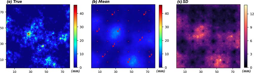
3822                                         J. Yan et al.: Conditional simulation of spatial rainfall fields using random mixing

2.2    Prepare the constraints

The simulation is embedded in Gaussian space; hence, the
constraints should be transformed to the standard normal
marginal (normalized Gaussian). Specifically, we consider
the following three constraints:

 1. The equality constraints at rain gauge locations, when
    defined in terms of the standard normal marginal, mean
    that the simulated values at the rain gauge locations
    should equal the values mapped from the rain gauge ob-
    servations rk :
                                                                      Figure 2. The blue lines denote the empirical variograms evaluated
                  −1                                                  from 1000 truncated Gaussian fields; the 95 % confidence interval
      Z (xk ) = 8      (G (rk )) for k = 1, . . ., K,         (1)
                                                                      is marked by the black dashed lines. The red line denotes the true
      where Z is the simulated Gaussian field, xk denotes the         variogram used to generate the continuous Gaussian fields. Note
                                                                      that the continuous Gaussian field is truncated at z0 = 8−1 (0.36).
      rain gauge location, and G(·) and 8(·) denote the rain-
      fall CDF and the CDF of the standard normal distribu-
      tion, respectively.                                               3. The pattern of the simulated field should resemble that
 2. The simulated Gaussian field Z should preserve a given                 of the radar estimates as closely as possible. This repre-
    correlation function obtained from the transformed                     sents an optimization problem, and the goal is to maxi-
    radar estimates, i.e.                                                  mize the Pearson correlation coefficient of the simulated
                                                                           field Z and the reference field Zr0 , i.e.
      Zr0 = 8−1 (G (Rr )) .                                   (2)
                                                                           O(Z) = ρ Z, Zr0 → max,

                                                                                                                                  (3)
      The problem here is that one can only obtain a trun-
      cated Gaussian field Zr0 from the radar estimates Rr , as             where Z is the simulated Gaussian field, Zr0 is obtained
      all the dry pixels in Rr are converted to z0 = 8−1 (u0 ),             from the radar estimates as defined in Eq. (2), and ρ(·) is
      where u0 is the spatial intermittency. The sill of the cor-           the Pearson correlation coefficient. The same problem
      relation function evaluated from Zr0 is reduced due to                arises: Z is continuous whereas Zr0 is truncated. To eval-
      the truncation. Figure 2 displays and compares empiri-                uate the objective function, one could truncate Z at z0 or
      cal variograms evaluated from 1000 truncated Gaussian                 one could also use Z directly, as shown in Eq. (3). The
      fields with the true variogram used to generate the corre-            difference between these approaches is minor, as a high
      sponding continuous Gaussian fields. From the figure, it              correlation between Zr0 and Z means a high correlation
      can be seen that the empirical and true variograms have               between Zr0 and the truncated Z. To be as parsimonious
      very similar patterns. Practically speaking, the true cor-            as possible, we use Z directly in the evaluation of the
      relation function can be approximated by scaling given                objective function.
      a priori knowledge that the variance of the simulated
      field is 1. Besides, as random mixing is a geostatistical       2.3   Random mixing
      simulation method, the choice of the correlation func-
      tion has a limited effect on the estimates, just as it does     The task is to estimate the true rainfall field given a set of
      for Kriging (Verworn and Haberlandt, 2011). We denote           rain gauge observations and a set of radar estimates. In terms
      the estimated correlation function by 0 hereafter.              of conditional simulation, this means simulating a Gaussian
      Note that the terms correlation function and variogram          field Z that fulfils all the constraints described in Sect. 2.2
      are used interchangeably here, as it is common in geo-          and then converting Z to the rainfall field of interest, i.e.
      statistics to work with the variogram, the estimation           yielding an estimate of the true rainfall field.
      of which has been shown to be more stable than that                We use random mixing (RM) to fulfil the task. RM utilizes
      of the correlation function (Calder and Cressie, 2009).         the concept described in Hu (2000): that the conditional field
      Namely, one simulates by using the correlation function         of interest can be obtained as a linear combination of many
      as the measure of spatial dependence, whereas the spa-          unconditional random fields, i.e.
      tial dependence of the simulated field is normally exam-
                                                                            N
      ined via its variogram.                                         Z=
                                                                            X
                                                                                  αi Yi ,                                            (4)
                                                                            i=1

Hydrol. Earth Syst. Sci., 25, 3819–3835, 2021                                               https://doi.org/10.5194/hess-25-3819-2021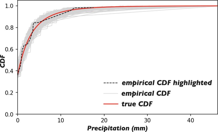
J. Yan et al.: Conditional simulation of spatial rainfall fields using random mixing                                                              3823

                                                                                                                            N
where Yi (s) are independent Gaussian random fields with                               In addition, the constraint
                                                                                                                            P
                                                                                                                                  αi2 < 1 is imposed to
identical statistical properties, i.e. the marginal distributions                                                           i=1
all follow the standard normal distribution with the same                              ensure Pthat the second part has a positive weight,
correlation function. If, in addition, the L2 norm of the                              i.e. 1− αi2 > 0. The extra constraint is further sat-
weights αi fulfils                                                                     isfied by increasing N , i.e. increasing the number of
                                                                                       degrees of freedom of the equation system.
N
X
      αi2 = 1,                                                              (5)     b. The second part,
i=1                                                                                                                q    X
                                                                                       (cos θ · H + sin θ · H 0 ) · 1 −   αi2 ,
the resultant conditional field Z is statistically identical to Yi ,
as demonstrated by Bárdossy and Hörning (2016). There are                              is made up of two independent, statistically identi-
several methods that can be used to obtain Gaussian random                             cal conditional random fields H and H 0 , which are
fields with a given correlation function. We have used an ef-                          referred to as the H -field hereafter. The H -field is
ficient method – the fast Fourier transform for regular grids                          also obtained as a linear combination of uncondi-
(Wood and Chan, 1994; Wood, 1995; Ravalec et al., 2000).                               tional random fields Yi0 (statistically identical to Yi ):
   It is necessary to differentiate Hu’s method from the pro-
posed one before specifying the algorithm. Hu’s method (Hu,                                   M
                                                                                              X
2000; Hu et al., 2001) incorporates linear data using condi-                           H=            βi Yi0 .
                                                                                               i=1
tional Kriging, and the method is extended to combine de-
pendent conditional fields in Hu (2002), whereas RM incor-                             The H -field is special because of the zeros at the
porates linear or nonlinear constraints under the unified con-                         rain gauge locations, which mean that the addition
cept of randomly mixing unconditional random fields. The                               of the second part to the first part does not change
algorithm for RM is as follows:                                                        the values at the rain gauge locations. Hence, the
                                                                                       equalities in Eq. (7) can be rewritten as
  1. The prospective conditional Gaussian field Z that fulfils
     all the constraints is obtained as                                                              N
                                                                                                     X
            N                                            q                             Z (xk ) ≡           αi · Yi (xk ) + 0 = 8−1 (G (rk ))
            X                                                      X
       Z=         αi Yi +(cos θ ·H +sin θ ·H 0 )· 1 −                  αi2 . (6)                     i=1

            i=1                                                                                      for k = 1, . . ., K.                           (8)
       Z consists of two parts:                                                        The remaining question is how to obtain such H -
                                                                                       fields. Similarly, an underdetermined system is cre-
        a. The first part,
                                                                                       ated as
            N
            X                                                                          M
                  αi Yi ,
                                                                                       X
                                                                                             βi · Yi0 (xk ) = 0 for k = 1, . . ., K,                (9)
            i=1                                                                        i=1

            is made up of N statistically identical unconditional                      with M unknowns, K equations, and M > K. To
            random fields Yi (s) with correlation function 0, as                       ensure that the H -field is statistically identical to Y 0
            estimated in Sect. 2.2. The role of this part is to                        (or Y ), the following constraint is imposed addi-
            fulfil the equality constraints at the rain gauge loca-                    tionally:
            tions. Thus, K linear constraints are imposed as
                                                                                       M
                                                                                       X
            N
            X
                                      −1
                                                                                             βi2 = 1.                                             (10)
                  αi · Yi (xk ) = 8        (G (rk )) for k = 1, . . ., K. (7)          i=1
            i=1
                                                                                       The set of weights (βi for i = 1, . . . , M) can be de-
            See Eq. (1) for the definitions of xk , rk , G(·) and                      termined by solving Eq. (9) first,   and then scaling
            8−1 (·). In total, we have N unknowns: αi for i =                                                           qP
            1, . . . , N and K equations. If N > K, this forms an                      the weights with the factor (1/           βi2 ) such that
            underdetermined equation system. Multiple tech-                            Eq. (10) is satisfied. Because of the “zeros”, scal-
            niques are available for solving such a system.                            ing does not change the values at the rain gauge
            Specifically, we found the set of weights with the                         locations.
                                                  N
                                                     αi2 by using
                                                  P
            lowest L2 norm; i.e. we minimized                                      The Gaussian field Z obtained from Eq. (6) fulfils the
                                                             i=1                   equality constraints at the rain gauge locations and re-
            the singular value decomposition technique.                            produces the correlation function 0. The correlation

https://doi.org/10.5194/hess-25-3819-2021                                                    Hydrol. Earth Syst. Sci., 25, 3819–3835, 2021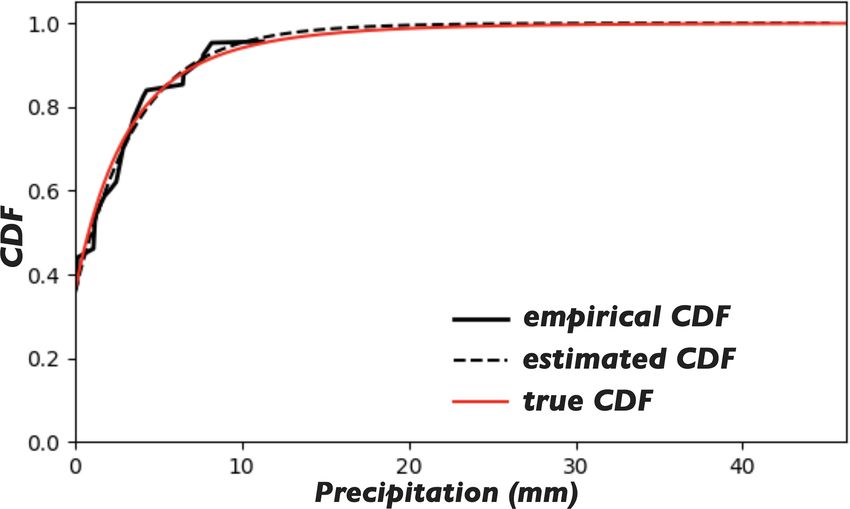
3824                                       J. Yan et al.: Conditional simulation of spatial rainfall fields using random mixing

    function is reproduced because the L2 norm of the               3     Data
    weights of all the fields underlying Z satisfies
    X                              X                            An artificial experiment was carried out to test the capabil-
       αi2 + cos2 θ + sin2 θ · 1 −        αi2 = 1.   (11)           ity of the proposed approach to estimate the true rainfall
                                                                    field. Due to a lack of knowledge of the true fields, we used
    It should be noted that one H -field is sufficient to do the    synthetic ones: 1000 rainfall fields were generated indepen-
    same job. For example, one could obtain such a Z via            dently and served as the “true” rainfall fields from which the
           N                q                                       radar and rain gauge data were derived.
           X                     X
    Z=           αi Yi + H · 1 −   αi2 .                               This was done because it is difficult to verify the accu-
           i=1                                                      racy of the estimates comprehensively without knowing the
                                                                    real rainfall field. Some studies employ the leave-n-out cross-
    The aim of using two H -fields instead of one is to intro-
                                                                    validation method, where one verifies the accuracy of the es-
    duce more freedom, allowing the third constraint  qPto be       timates at certain points, for verification. However, the accu-
    met too. The relative weights of the two parts (      αi2 :     racy of the estimates in terms of the overall statistics (e.g. the
                                                                    mean and maximum of the rainfall field) is more hydrologi-
    q
      1 − αi2 ) do matter. The second part should weigh
          P
                                                                    cally interesting than the accuracy at particular points.
    more, as this facilitates the solution of the optimization
    problem defined in the next step. Thus, when solving            3.1     Generate the true rainfall fields
    the
    qPunderdetermined system in (a), the set of weights
         αi2  1 is found.                                          1000 rainfall fields, each with a grid size of 80 × 80, were
                                                                    generated. Each pixel was assumed to represent an area of
 2. Due to the freedom introduced by the extra H -field, the        1 × 1 km2 , and all 1000 fields were generated independently
    Gaussian field Z obtained from Eq. (6) is a function of         and had identical properties, i.e. they all had the same spa-
    θ . This is also true of the objective function evaluated       tial intermittency, rainfall CDF, and correlation function. The
    from Z, which actually defines a 1D optimization prob-          generation procedure was as follows:
    lem w.r.t. θ :
                                                                        1. Generate 1000 Gaussian random fields ZT with a given
    O(θ ) = ρ Z(θ ), Zr0 → max,

                                                         (12)              correlation function. Figure 3a displays the exponential
                                                                           correlation function used in the generation of ZT . Note
    where θ ∈ (−π, π ]. See the definitions of Zr0 and ρ(·) in
                                                                           that a subscript T is used throughout this paper to denote
    Eqs. (2) and (3). The task is to find the θ that produces
                                                                           the true Gaussian and rainfall fields or the true rainfall
    the maximum objective function value. There are vari-
                                                                           CDF. Similarly, we used the fast Fourier transform for
    ous methods that can be applied to solve the 1D uncon-
                                                                           regular grids to generate ZT .
    strained optimization problem. In this work, we simply
    used the trial-and-error method, and a coarse search fol-           2. Generate a rainfall CDF where the lognormal distribu-
    lowed by a fine search was implemented to accelerate                   tion is used as the model for the rainfall CDF, as this
    the solving process. The solution to the 1D optimiza-                  distribution has been shown to be effective at describing
    tion problem is denoted by θ ∗ .                                       the marginal distribution of rainfall rates or the short-
                                                                           time rainfall (accumulation time: 10 or 15 min) over a
 3. If Z(θ ∗ ) meets the stopping criterion of the optimiza-
                                                                           specified area (Bell, 1987; Crane, 1990; Pegram and
    tion, continue with step 4. Otherwise, go back to step 2
                                                                           Clothier, 2001). Figure 3b shows the rainfall CDF used
    after updating H and H 0 as follows:
                                                                           in the generation of the 1000 true rainfall fields, i.e. the
    H ← cos θ · H + sin θ · H 0                            (13)            true rainfall CDF: G−1
                                                                                                T (·).
       0
    H ← a newly generated H -field.                        (14)         3. Convert the Gaussian random fields ZT to rainfall fields
    As always in optimization, there are multiple choices of               using the normal-score transformation method:
    stopping criteria, such as a particular number of itera-
                                                                           RT = G−1
                                                                                 T (8 (ZT )) ,                                    (16)
    tions, a preset limit on the objective function, a specific
    rate of decrease of the objective function, and so forth.              where RT is the true rainfall field and 8(·) is the CDF
    We adopted a specific number of continuous iterations                  of the standard normal distribution. Note that the quan-
    without improvement as the stopping criterion.                         tile value u0 , which is labelled in Fig. 3b, is used to
 4. Finally, an estimate of the true rainfall field is obtained            maintain the spatial intermittency. Hence, all pixel val-
    as                                                                     ues smaller than z0 = 8−1 (u0 ) in ZT are converted to
                                                                           zero (precipitation) in RT .
    R = G−1 8 Z θ ∗ .

                                                           (15)

Hydrol. Earth Syst. Sci., 25, 3819–3835, 2021                                          https://doi.org/10.5194/hess-25-3819-2021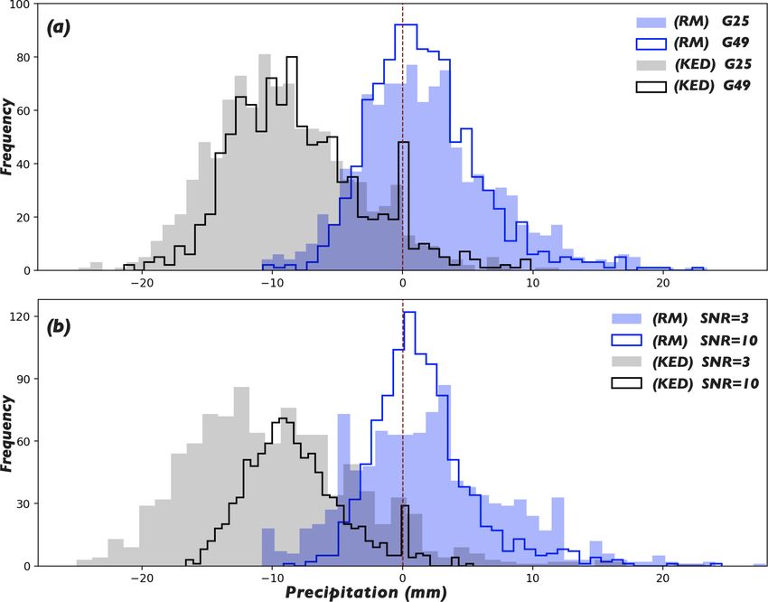
J. Yan et al.: Conditional simulation of spatial rainfall fields using random mixing                                              3825

                                                                           The proposed approach was tested at three levels of sig-
                                                                           nificance: SNR = 3, 5, and 10. Accordingly, the Gaus-
                                                                           sian fields with introduced random error were obtained
                                                                           as

                                                                           Zr = 0.9487 · ZT + 0.3162 · Ze
                                                                           Zr = 0.9806 · ZT + 0.1961 · Ze
                                                                           Zr = 0.9850 · ZT + 0.0985 · Ze .

                                                                        2. Convert the Gaussian fields with random error to rainfall
                                                                           fields using the normal-score transformation:

                                                                           Rr = G−1
                                                                                 T (8 (Zr )) .                                     (18)

                                                                           The resultant Rr differs in pattern from the true rain-
                                                                           fall field, while differences in statistical properties are
                                                                           small. See the statistical properties evaluated from the
                                                                           true rainfall field and the rainfall fields that contain ran-
                                                                           dom error only (i.e. the rainfall fields obtained via per-
Figure 3. (a) The exponential correlation function used in the gen-        forming steps 1 and 2 in Fig. 4.
eration of the Gaussian random fields ZT . (b) The rainfall CDF
used in the generation of the true rainfall fields, where the spatial   3. Apply a nonlinear transformation to mimic the error
intermittency u0 is labelled.                                              induced through the use of an erroneous Z–R rela-
                                                                           tionship. In practice, the true Z–R relationship is dif-
                                                                           ficult to identify. The omnipresent Z–R relationship
                                                                           Z = 200R 1.6 given by Marshall and Palmer (1948) is
                                                                           widely used in radar hydrology to convert radar reflec-
3.2   Generate the radar estimates                                         tivity to rain rate. Long lists of vastly different Z–R re-
                                                                           lationships have been derived for different areas with
The radar estimates were derived from the true rainfall fields.            different conditions in the scientific literature (Uijlen-
Specifically, the Gaussian field ZT generated in Sect. 3.1 was             hoet, 2001; Fabry, 2015). However, the Z–R relation-
used. Two types of errors are commonly seen in radar es-                   ship varies over space and time. Generally, there is no
timates: random and nonlinear errors. The following proce-                 means to identify the true Z–R relationship in real time.
dure was applied to mimic those errors:                                    In other words, most of the time, an erroneous Z–R
                                                                           relationship is employed, which results in a nonlinear
  1. Introduce a random error. The proposed approach as-                   departure of the radar estimates from the true rainfall
     sumes that the radar estimates measured aloft can rep-                field: the larger the radar measurement, the more seri-
     resent the pattern of the rainfall field on the ground.               ous the departure. Given the above, we used the follow-
     However, there are some factors that can reduce the rep-              ing power function to mimic this nonlinear departure
     resentativeness of radar estimates, such as evaporation,              (where the operator “←” denotes updating):
     complex terrain effects, and anthropogenic effects. A
     random error is therefore introduced to mimic this kind               Rr ← 0.87Rr0.83 .                                       (19)
     of error. We also utilize the concept of random mixing,
     where the Gaussian field with the introduced random                   The values of the two parameters – the factor of 0.87
     error is obtained by mixing two fields:                               and the exponent of 0.83 – are selected arbitrarily, as
                                                                           these values do not influence the proposed approach
      Zr = w1 · ZT + w2 · Ze ,                                  (17)       where the transformed radar estimates (the radar quan-
                                                                           tiles) are utilized. The monotonic transformation above
      where ZT is the true Gaussian field and Ze is an in-                 does not change the quantile map. We modelled a case
      dependently generated Gaussian random field with the                 where radar underestimates the precipitation, as this is a
      same statistical properties as ZT . The constraint w12 +             known tendency of radar data (Curry, 2012; Berne and
      w22 = 1 is also imposed to ensure that the resultant Zr              Krajewski, 2013; Shehu and Haberlandt, 2020). Under-
      is statistically identical to ZT (or Ze ). The ratio of the          estimated precipitation is useless and can have negative
      two weights (w1 /w2 ) is used to measure the signif-                 effects in many hydrological applications. On the other
      icance of the random error, by analogy with a com-                   hand, the choice of values for the two parameters does
      monly seen parameter, the signal-to-noise ratio (SNR).               matter for radar–gauge merging techniques, where the

https://doi.org/10.5194/hess-25-3819-2021                                          Hydrol. Earth Syst. Sci., 25, 3819–3835, 2021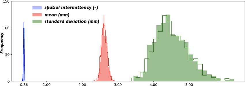
3826 J. Yan et al.: Conditional simulation of spatial rainfall fields using random mixing
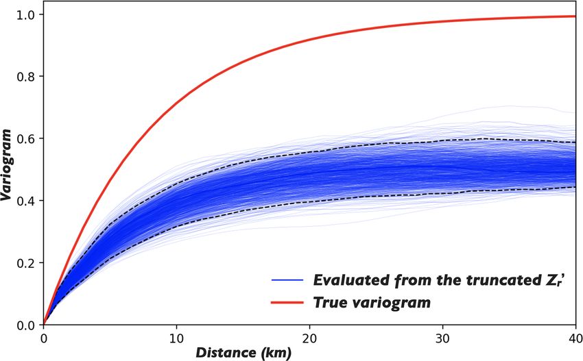
radar estimates are used directly. Thus, underestimated 2. The estimates from KED and conditional merging cap-
radar estimates lead to underestimated precipitation, for ture the pattern but neither possess the extremes of the
example. true field. KED outperforms conditional merging in this
case because KED takes the radar estimates as the ex-
ternal drift and tries to capture the linear relationship
3.3 Generate the rain gauge observations
between the gauge observations and the radar estimates
The rain gauge observations were sampled from the true rain- at the gauge locations. Thus, the estimates from KED
fall field RT at the rain gauge locations. Due to the local ef- correct the extremes of the radar estimates a little bit
fect of the rain gauge observations (the closer an ungauged but not perfectly, as radar underestimates the rainfall
location is to its nearest rain gauge, the less uncertain the cor- field nonlinearly in the scenario considered. In this spe-
responding estimate is), it is favourable to have a denser rain cific case, the maximum values in the true and KED-
gauge network. However, it is always an interesting question estimated rainfall fields are 46.24 and 32.55 mm, re-
to ask how dense the rain gauge network must be to achieve spectively. Compared to KED, conditional merging is
sufficient accuracy. We try to answer this question in the ex- more dependent on the accuracy of the radar estimates,
perimental context of this study. As it would have been too as the method assumes that the radar data provide an es-
complex to model real-world rain gauge networks, which are timate of the actual Kriging error. As KED outperforms
usually irregularly distributed and have various densities, we ordinary Kriging and conditional merging in this con-
made things as simple as possible. The proposed approach text, the results from RM are compared with those from
was tested on three layouts: 5×5, 6×6, and 7×7 rain gauges KED in the following subsections.
that are uniformly distributed in the domain of interest (de- 3. The rainfall field obtained from RM captures the ex-
noted G25, G36, and G49, respectively, hereafter). Presum- tremes of the true field. The maximum values in the
ably, this gives an approximate coverage of one rain gauge true and RM-estimated rainfall fields are 46.24 and
per 256, 178, and 131 km2 , respectively. 47.57 mm, respectively. The pattern of the true field is
captured with limited accuracy. After analysing the re-
4 Results sults from RM further, it is found that:
3.1. The proposed approach is capable of capturing the
4.1 Comparison of the results
extremes of the true field under the condition that
The proposed approach (referred to simply as RM in this sec- the estimated rainfall CDF is relatively accurate;
tion, though RM is in fact only part of the approach) was used see the estimated and true CDFs for the specific
to estimate the 1000 true rainfall fields based on the corre- case in Fig. 6.
sponding radar estimates and rain gauge observations. The 3.2. Unlike the estimates from ordinary Kriging, KED,
results from RM were compared with those from three well- or conditional merging, where one obtains a Kriged
known Kriging methods: ordinary Kriging, Kriging with ex- mean field, the proposed approach can yield an in-
ternal drift (KED), and conditional merging (Sinclair and Pe- finite number of realizations for the same true rain-
gram, 2005). It is not possible to display all the results ob- fall field due to the Monte Carlo framework. The
tained in this paper; we focus on the results for one rainfall mean of 100 realizations is displayed in Fig. 7b;
field randomly drawn from a total of 1000. A single realiza- this should be compared with the true rainfall field
tion obtained from RM is shown in Fig. 5b, which should shown in Fig. 7a. From the figure, it can be seen that
be compared with the corresponding true rainfall field and the mean realization is smooth and captures the pat-
the radar estimates presented in Fig. 5a and c, respectively. tern of the true field; in other words, the rain cells
Meanwhile, the estimates obtained from ordinary Kriging, are more accurately located in the mean realiza-
KED, and conditional merging are displayed in Fig. 5d–f, tion than in the individual realization. However, the
respectively. The results shown here are typical enough to statistics of the mean realization (variance and co-
be able to draw the following conclusions (conclusion 1 for variance) are clearly different from those of the true
ordinary Kriging, 2 for KED and conditional merging, and field. In summary, the individual realization gives
3 for RM): relatively accurate statistics; an ensemble of such
realizations is an accurate indicator of the locations
1. The rainfall field obtained from ordinary Kriging has of rainfall peaks. When feeding such an ensemble
neither the pattern nor the extremes of the true rainfall to applications such as a hydrological model, for
field, as the method only considers the rain gauge ob- example, one will also obtain an ensemble of esti-
servations; the radar estimates do not contribute to the mates, meaning that the estimation uncertainty for
final estimates. the rainfall field will propagate.
Hydrol. Earth Syst. Sci., 25, 3819–3835, 2021 https://doi.org/10.5194/hess-25-3819-2021J. Yan et al.: Conditional simulation of spatial rainfall fields using random mixing 3827
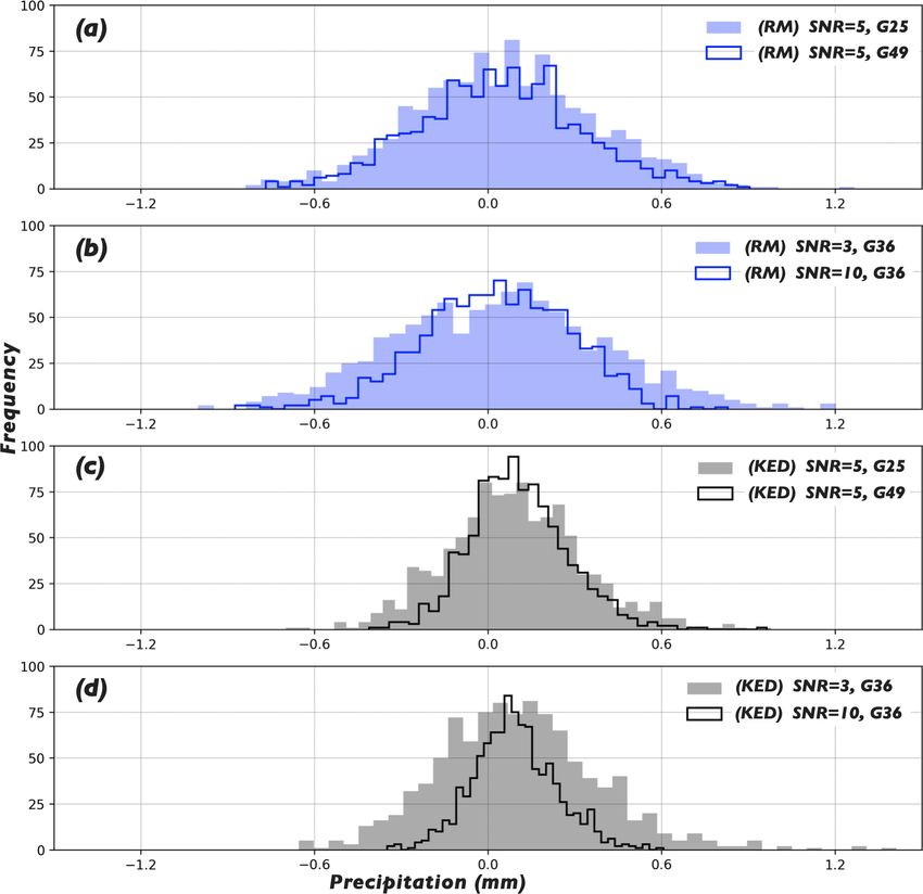
Figure 4. The coloured histograms were evaluated from the 1000 true rainfall fields. The unfilled histograms overlaid on the coloured ones
were evaluated from the 1000 rainfall fields that contain random error only (SNR = 3).
Figure 5. (a) The true rainfall field; (b) a single realization from RM (scenario: G36, SNR = 3); (c) the radar estimates; (d–f) the estimates
obtained from ordinary Kriging, Kriging with external drift (KED), and conditional merging, respectively.
3.3. The various estimates from RM provide a reason- side) and (b) the expected estimate at the pixel (i.e.
able representation of the estimation uncertainty. the uncertainty from the radar side). There is a clear
Figure 7c displays the standard deviation (std) of tendency: the closer the pixel to the neighbouring
the 100 realizations. The black/zero-valued 6 × 6 rain gauge and the smaller the expected estimate at
pixels (which are uniformly distributed in the do- the pixel, the lower the estimation uncertainty at the
main) reveal the locations of the rain gauges, as all pixel.
the realizations present the same values at these lo-
cations. The exact locations of the rain gauges are To show the estimation uncertainty at different pix-
marked by the small red dots in Fig. 7b. Compared els, the box and whisker plots for nine selected pix-
to the Kriging variance, which reflects the relative els are displayed in Fig. 8. The locations and IDs of
positions of the unknowns and the data points only, the nine pixels are given in Fig. 7b. It can be seen
the std map from RM is more physically meaning- from the figure that the true values of the 9 px all
ful. The estimation uncertainty of a pixel is affected fall in the central boxes, i.e. within the interquar-
by two factors: (a) the distance of the pixel from tile range (IQR). Among the 9 px, pixels 3, 4, and
the data points (i.e. the uncertainty from the gauge 8 are collocated with the rain gauges, and all the
estimates at those 3 px equal the true values, which
https://doi.org/10.5194/hess-25-3819-2021 Hydrol. Earth Syst. Sci., 25, 3819–3835, 20213828 J. Yan et al.: Conditional simulation of spatial rainfall fields using random mixing
20 realizations for each true field and use the median of the
20 errors – the difference between the simulated and true
maxima for each realization – as the representative. Figure 9
shows histograms of the errors w.r.t. the estimated field max-
ima for the 1000 fields obtained by RM and KED. Specifi-
cally, the upper panel shows the influence of the rain gauge
layout and the lower panel shows the influence of the level of
random error in the radar estimates. For the sake of clarity,
we only display the scenarios with the most and least rain
gauges (i.e. G25 and G49) in the upper panel, with the ran-
dom error in the radar estimates fixed at SNR = 5. Similarly,
Figure 6. The solid and dashed black lines show the empirical and in the lower panel, only the results of the scenarios with the
estimated rainfall CDFs for the specific case shown in Fig. 5b. The largest and smallest levels of random error in the radar es-
red line shows the true rainfall CDF used in the generation of the timates (i.e. SNR = 3 and 10) are displayed, with the rain
true fields. gauge layout fixed at G36. It can be seen from the figure that
there are negative biases in all the results from KED, while
the biases of the results from RM are not obvious. Further,
demonstrates the fulfilment of the equality con-
it can be seen that increasing the number of rain gauges and
straints at the rain gauge locations directly. Pixels 1
reducing the level of random error in the radar estimates are
and 2 are distant from their nearest rain gauges, but
both beneficial to the quality of the estimates, i.e. they reduce
those two pixels are located in regions where less
the size of the error and decrease the estimation variance (re-
rainfall is expected. Thus, the estimates at the 2 px
duce the scatter in the histogram).
present relatively low variance. Pixels 5, 7, and 9
The histogram shown in Fig. 9 can be summarized by two
are also distant from their nearest rain gauges, but
statistics: the mean error (ME) and the interquartile range
those 3 px are located in regions where more rain-
of the errors (IQR, the range between the quantiles 0.75
fall is expected. Thus, the corresponding estimates
and 0.25). Table 1 shows the two statistics evaluated from
present higher variance. Though pixel 6 is close to
the results for all the scenarios. It can be seen from the upper
its nearest rain gauge, it is located in a region where
part of the table that the estimates from RM are slightly over-
much rainfall is expected. Thus, the corresponding
estimated, and that the estimates from KED are significantly
estimates show relatively high variance.
underestimated. For both methods, increasing the number of
4.2 Sensitivity analysis rain gauges and reducing the level of random error in the
radar estimates help to reduce the ME and shrink the IQR.
The accuracy of the estimates is mainly affected by two fac- Yet for RM, more is not necessarily better. For example, the
tors: the number of rain gauge observations and the random best performance in terms of ME and the best performance
error in the radar estimates. To analyse the influence of the in terms of IQR both occur in scenario (SNR = 10, G36).
two factors, the 1000 true rainfall fields were estimated under Scenario (SNR = 10, G49) – which is assumed to perform
different scenarios: radar estimates with different levels of the best – is only ranked second, possibly due to the overfit-
random error (SNR = 3, 5, and 10) and rain gauge networks ting problem in the estimation of the rainfall CDF. When the
with different layouts (5 × 5, 6 × 6, and 7 × 7 rain gauges radar estimates are relatively accurate, the presence of a cer-
that are uniformly distributed in the domain; these were de- tain number of rain gauges is enough to sample sufficient in-
noted G25, G36, and G49, respectively). Specifically, we fo- formation. Increasing the number of rain gauges further can
cus on two statistics when evaluating the estimation accu- lead to the overfitting problem, due to the surplus of infor-
racy: the mean and maximum of the estimated rainfall field. mation.
The former is noteworthy when the estimated rainfall field is
used in studies where the water balance of a region is impor- 4.2.2 Field mean
tant; the latter is of great importance when the extreme for
the region is of interest (e.g. for stormwater management or The estimated mean of the rainfall field by RM or KED is
flood risk assessment). compared with the true mean to evaluate the accuracy in
terms of the mean statistic. For each of the 1000 true fields,
4.2.1 Field maximum an ensemble of 20 realizations is produced by RM and the
mean of the 20 errors – the difference between the simu-
The maximum of the rainfall field obtained from RM or lated and the true means for each realization – is used as the
KED is compared with the true maximum. Using RM, one representative. Figure 10 shows the histograms of the errors
could obtain an infinite number of realizations for each of w.r.t. the estimated field means for the 1000 fields obtained
the 1000 true rainfall fields, so we simulate an ensemble of from RM in Fig. 10a and b and from KED in Fig. 10c and d.
Hydrol. Earth Syst. Sci., 25, 3819–3835, 2021 https://doi.org/10.5194/hess-25-3819-2021J. Yan et al.: Conditional simulation of spatial rainfall fields using random mixing 3829
Figure 7. (a) The true rainfall field; (b) the mean of 100 realizations obtained from RM (the small red dots denote the locations of the rain
gauges, and the red triangles labelled with IDs denote the 9 px selected to develop the box and whisker plots shown in Fig. 8); (c) the standard
deviation (std) of the 100 realizations.
Figure 8. Box and whisker plots of the estimates at nine selected pixels (see the locations and IDs of the 9 px in Fig 7b). The blue dots denote
the true values, i.e. the values at the corresponding pixels in the true field.
Table 1. The mean error (ME) and the interquartile range (IQR) of For KED, the influences of the two factors are ambiguous.
the errors w.r.t. the estimated field maxima for the 1000 true rainfall Increasing the number of rain gauges or reducing the level of
fields obtained by RM (the three columns on the left) and by KED random error in the radar estimates helps to reduce the esti-
(the three columns on the right). The column name denotes the SNR mation variance, but it is unclear whether it helps to reduce
of the radar estimates whereas the row name denotes the rain gauge the size of the error. For RM, neither the influences of the
layout.
two factors nor the biases in the estimates are obvious.
We still use the two statistics – ME and IQR – to gen-
ME 3 5 10 3 5 10
eralize each histogram, and the results for all the scenarios
G25 2.182 1.929 1.611 −10.114 −9.104 −8.741 are shown in Table 2. It can be seen from the upper part of
G36 1.819 1.698 1.451 −9.760 −8.700 −8.250
the table that RM outperforms KED in terms of the ME, as
G49 1.740 1.611 1.538 −8.997 −7.960 –7.620
the MEs from RM in all the scenarios are smaller than the
IQR RM KED best performance of KED. It is worth considering that, based
G25 9.551 6.497 4.798 9.650 7.166 5.312 on the previous analysis, KED is expected to underestimate
G36 7.742 5.574 4.218 8.703 6.539 4.624 the maximum of the rainfall field; however, the results shown
G49 6.665 5.057 4.242 8.652 6.684 5.101 here indicate that KED overestimates the mean of the field.
The best performances in terms of the ME and IQR for both methods are printed in bold. KED is therefore likely to overestimate the lower quantiles
of the rainfall field. Further, the table also demonstrates that
RM is not very sensitive to the two factors in terms of the
It can be seen from the figure that, compared to RM, KED mean statistic, as one can see barely any trend.
seems to be more sensitive to the two factors. Further, slight
positive biases can be observed in the estimates from KED
for all the displayed scenarios. Among the four subfigures,
Fig. 10a and c show the influence of the rain gauge layout
for RM and KED, respectively, while Fig. 10b and d show the
influence of the level of random error in the radar estimates.
https://doi.org/10.5194/hess-25-3819-2021 Hydrol. Earth Syst. Sci., 25, 3819–3835, 20213830 J. Yan et al.: Conditional simulation of spatial rainfall fields using random mixing
Figure 9. Histograms of the errors w.r.t. the estimated field maxima for the 1000 true rainfall fields obtained by RM and KED. (a) The results
for the scenarios with different rain gauge layouts, with the random error in the radar estimates fixed at SNR = 5. (b) The results for the
scenarios with different levels of random error in the radar estimates, with the rain gauge layout fixed at G36.
Table 2. The mean error (ME) and the interquartile range (IQR) of the CDF method hereafter) and the method of random mix-
the errors w.r.t. the estimated field means for the 1000 true rainfall ing (RM), which is used to simulate random spatial fields
fields obtained by RM (the three columns on the left) and by KED under constraints.
(the three columns on the right). The column name refers to the The CDF method provides the foundation for the ap-
SNR of the radar estimates, and the row name denotes the layout of proach. A resultant rainfall CDF with sufficient accuracy
the rain gauges.
is necessary for the successful application of the approach.
The statistics of intermittent precipitation are not Gaussian,
ME 3 5 10 3 5 10
which restricts the usage of well-established stochastic mod-
G25 0.049 0.055 0.023 0.103 0.090 0.082 els that assume Gaussianity (Pulkkinen et al., 2019). Specif-
G36 0.038 0.033 0.029 0.105 0.096 0.092 ically in this study, the rainfall CDF is important in two re-
G49 0.038 0.039 0.030 0.116 0.106 0.099 spects: (a) it is used in the data transformation, whereby the
IQR RM KED simulated Gaussian fields are transformed into rainfall fields
of interest; (b) it is used to define the constraints in terms of
G25 0.545 0.412 0.340 0.434 0.300 0.212 the normalized Gaussian marginal.
G36 0.490 0.372 0.352 0.355 0.251 0.182
RM, on the other hand, is an excellent tool that performs
G49 0.438 0.362 0.353 0.294 0.214 0.154
conditional simulation in Gaussian space, but it is not ir-
The best performance levels in terms of the ME and IQR for each method are replaceable. Another conditional simulation method could
printed in bold.
have been used, such as phase annealing (Yan et al., 2020).
RM was employed in this study due to (a) its relatively high
5 Discussion efficiency, which makes the mass production of realizations
possible, and (b) code availability (a Python package for the
5.1 The two core components of the approach conditional simulation of random spatial fields using RM is
available, with the authors giving practical demonstrations of
In this paper, an approach allowing estimates of spatial rain- the application of the method; Hörning and Haese (2021)).
fall fields to be obtained together with the associated uncer-
tainty is proposed. This approach has two core components:
the method used to compute the rainfall CDF (referred to as
Hydrol. Earth Syst. Sci., 25, 3819–3835, 2021 https://doi.org/10.5194/hess-25-3819-2021J. Yan et al.: Conditional simulation of spatial rainfall fields using random mixing 3831
Figure 10. Histograms of the errors w.r.t. the estimated field means for the 1000 true rainfall fields obtained by RM (a, b) and KED (c, d).
The estimates were obtained under different scenarios; see the text in the subfigures for the specific scenarios.
5.2 The scope of the approach used to perturb a deterministic nowcast (e.g. Liguori and
Rico-Ramirez, 2014; Foresti et al., 2016). The output of the
proposed approach – an ensemble of estimates that consid-
The proposed approach is intended for the estimation of spa- ers both radar and rain gauge data – could be used to per-
tial rainfall fields following a short accumulation time: 15, turb a deterministic model, and this ensemble of estimates
10, or even 5 min. The temporal aspects of QPE (quanti- is more hydrologically meaningful than a random perturba-
tative precipitation estimates) are outside the scope of this tion, which is used in many probabilistic nowcast models
study. Unlike the acquisition of QPF (quantitative precipi- (e.g. Bowler et al., 2006; Berenguer et al., 2011; Pulkkinen
tation forecasts) by e.g. a radar-based nowcast model when et al., 2019). Besides, precipitation exhibits spatial variabil-
modelling the temporal evolution of the rainfall field is of ity; hence, it is challenging to estimate spatial rainfall fields
interest, the spatial rainfall fields are obtained in a hind- in a deterministic manner, even in a hindcast mode. If the
cast mode in this study. This approach has great potential to nowcasting community can embrace the change from a de-
improve the quality of QPF. Shehu and Haberlandt (2020) terministic framework to a probabilistic one, a similar change
showed that one of the major factors that causes the pre- could also happen in the hindcasting community.
dictability loss of a nowcast model is the inability of radar to
capture the true rainfall field. The proposed approach could 5.3 Concerning the CDF method
therefore be used to improve the rainfall field fed into the
model. 5.3.1 Basic assumption
Furthermore, radar-based nowcasting has evolved from the
use of a deterministic to the use of a probabilistic framework The rainfall CDF is computed from a set of rain gauge obser-
to estimate the predictive uncertainty (e.g. Pierce et al., 2012; vations and the radar estimates. The basic assumption of the
Shehu and Haberlandt, 2020). A common approach is based method is that the radar estimates can represent the pattern of
on stochastic simulation, in which correlated noise fields are the rainfall field to a reasonable extent. Random error, which
https://doi.org/10.5194/hess-25-3819-2021 Hydrol. Earth Syst. Sci., 25, 3819–3835, 20213832 J. Yan et al.: Conditional simulation of spatial rainfall fields using random mixing
can reduce the representativeness of the radar estimates, is 0.36. Practically speaking, the choice of u0 has only a minor
accounted for, and the quality control steps in the algorithm influence on the performance. When u0 > 0.36 (i.e. a larger
are specifically designed to get rid of the negative effects of dry-area ratio), the point at which the rainfall CDF intersects
random error. However, the degradation of representative- the y axis moves up, and there are also more zero samples
ness due to systematic effects in the radar estimates (e.g. in both the radar and rain gauge data. When 0 < u0 < 0.36
range-dependent errors associated with the increasing height (i.e. a larger wet-area ratio), the point moves down and there
of the radar beam or increasing sampling volume as the dis- are fewer zero samples. This method is problematic if u0 = 0,
tance from the radar antenna increases) is not accounted for. i.e. the entire domain is wet. In that case, there is no (0, u0 )
Thus, quality control to get rid of systematic effects in the and the requirement (stated in step 4 in Sect. 2.1) that the
radar estimates is necessary. CDF passes through the point (0, u0 ) does not apply.
5.3.2 Impact of the distribution and number of rain 5.3.4 Applicability in terms of the spatial scale
gauge observations
The CDF method is valid for a limited spatial scale. As
The capability of the CDF method is affected by the distri- the spatial scale increases, the domain eventually becomes
bution and number of rain gauge observations. A uniform too large for a single CDF to represent all processes. The
distribution of rain gauge observations is not required, but limit on the spatial scale is related to factors such as rainfall
the gauge observations should not be too clustered, as it is regime, topography, and geography. However, because syn-
normally considered that one has a better chance of obtain- thetic datasets were used instead of realistic datasets in this
ing spatially representative samples from a relatively evenly study, it was not possible to derive any useful information re-
distributed rain gauge network. garding the limit on the spatial scale. A further study based
It is often the case that only small samples from irregularly on realistic datasets is therefore required.
distributed rain gauge stations are available for mesoscale
hydrological studies. Sufficient gauge–radar pairs (samples)
must be available if we are to obtain a rainfall CDF with ad-
6 Conclusions and outlook
equate accuracy. There are two ways to increase the sample
size: In this paper, an approach for simulating spatial rainfall fields
1. Increase the sample size in space. For small domains conditioned on radar and rain gauge data was proposed.
with only a few rainfall stations (say 10), it can be as- The approach has two core components: a method to com-
sumed that rain parcels move uniformly. Under this as- pute the marginal distribution function of the rainfall field,
sumption, one can displace the radar quantile map us- and random mixing, which conducts a conditional simula-
ing a vector that decreases the radar–gauge mismatch tion in Gaussian space. An artificial experiment was per-
(using the Spearman’s rank correlation as the measure, formed to test the efficiency of the proposed approach, and
for example) and then refind the gauge-respective quan- the results were compared with those from three commonly
tiles in the displaced quantile map. The result is 10 new used Kriging methods: ordinary Kriging, Kriging with exter-
pairs (rk , u0k ) for k = 1, . . . , 10, where u0k is the refound nal drift (KED), and conditional merging. The proposed ap-
radar quantile. Normally, a stack of such vectors (N) proach was found to outperform KED and conditional merg-
can be found, which results in 10 · N new samples. One ing, especially in the estimation of extremes. The estimates
should limit the domain size when applying the above yielded by the proposed approach differ from those provided
practice. This technique has been applied by Yan and by the other methods in two respects. First, unlike the Krig-
Bárdossy (2019) to find the empirical rainfall CDF for ing methods, where a Kriged mean field is obtained by mini-
a domain of size 19 × 19 km2 . mizing the estimation variance, the output of the approach is
an ensemble of estimates (realizations) with identical statis-
2. Increase the sample size in time. A fixed time window tics (mean, variance, correlation function, etc.) due to the
can be set by assuming a relatively stable distribution Monte Carlo framework. Each individual realization strictly
during the relevant time interval, and the gauge–radar fulfils the equality constraints at rain gauge locations and
pairs in the time window can be used in the calculation presents a field pattern that is similar to the radar estimates,
of the rainfall CDF. and an ensemble of such realizations provides a tendency to-
A combination of both practices can enrich the sample size wards the accurate locations of the rainfall peaks. Second, the
to a remarkable extent. various estimates from the proposed approach provide a rea-
sonable representation of the estimation uncertainty. In ad-
5.3.3 Impact of spatial intermittency dition to representing the relative positions of the unknowns
and the data points (i.e. the information and the associated
In this work, the performance of the CDF method was tested uncertainty from rain gauge data), which are also provided
for the hydrologically interesting spatial intermittency u0 = by the Kriging variance, the estimation uncertainty obtained
Hydrol. Earth Syst. Sci., 25, 3819–3835, 2021 https://doi.org/10.5194/hess-25-3819-2021You can also read