Dynamic motion monitoring of a 3.6 km long steel rod in a borehole during cold-water injection with distributed fiber-optic sensing
←
→
Page content transcription
If your browser does not render page correctly, please read the page content below

Solid Earth, 13, 161–176, 2022
https://doi.org/10.5194/se-13-161-2022
© Author(s) 2022. This work is distributed under
the Creative Commons Attribution 4.0 License.

Dynamic motion monitoring of a 3.6 km long steel rod in a borehole
during cold-water injection with distributed fiber-optic sensing
Martin Peter Lipus1 , Felix Schölderle2 , Thomas Reinsch1,a , Christopher Wollin1 , Charlotte Krawczyk1,3 ,
Daniela Pfrang2 , and Kai Zosseder2
1 GFZ   German Research Centre for Geosciences, Telegrafenberg, 14473 Potsdam, Germany
2 Hydrogeology    and Geothermal Energy, Technical University Munich, Arcisstr. 21, 80333 Munich, Germany
3 Institute for Applied Geosciences, Technical University (TU) Berlin, Ernst-Reuter-Platz 1, 10587 Berlin, Germany
a present address: Fraunhofer IEG, Fraunhofer Research Institution for Energy Infrastructures and Geothermal Systems IEG,

Am Hochschulcampus 1 IEG, 44801 Bochum, Germany

Correspondence: Martin Peter Lipus (mlipus@gfz-potsdam.de)

Received: 11 May 2021 – Discussion started: 6 July 2021
Revised: 27 September 2021 – Accepted: 8 November 2021 – Published: 19 January 2022

Abstract. Fiber-optic distributed acoustic sensing (DAS)          1   Introduction
data find many applications in wellbore monitoring such
as flow monitoring, formation evaluation and well integrity       Fiber-optic distributed sensing in borehole applications has
studies. For horizontal or highly deviated wells, wellbore        gained a lot of attention in recent years. Distributed temper-
fiber-optic installations can be conducted by mounting the        ature sensing (DTS) has been used to assess rock thermal
sensing cable to a rigid structure (casing/tubing) which al-      properties and locations of water-bearing fractures (e.g., Hur-
lows for a controlled landing of the cable. We analyze a cold-    tig et al., 1994; Förster et al., 1997). DTS was used to per-
water injection phase in a geothermal well with a 3.6 km long     form cement job evaluations and wellbore integrity analysis
fiber-optic installation mounted to a 3/4 in. sucker rod by       during and after production tests (e.g., Pearce et al., 2009;
using both DAS and distributed temperature sensing (DTS)          Bücker and Großwig, 2017). The performance of a bore-
data. During cold-water injection, we observe distinct vibra-     hole heat exchanger was monitored with DTS to evaluate the
tional events (shock waves) which originate in the reservoir      heat input along the wellbore and to measure the regenera-
interval and migrate up- and downwards. We use tempera-           tion time after a heat extraction period (Storch et al., 2013).
ture differences from the DTS data to determine the theoret-      While DTS has found its way as a standard tool for well-
ical thermal contraction and integrated DAS data to estimate      bore monitoring over the last 2 decades, the utilization of
the actual deformation of the rod construction. The results       distributed acoustic sensing (DAS) is still subject to many
suggest that the rod experiences thermal stresses along the       research questions. Johannessen et al. (2012) introduced the
installation length – partly in the compressional and partly      potential and capabilities for acoustic in-well monitoring ap-
in the extensional regime. We find strong evidence that the       plications based on DAS systems which range from, e.g.,
observed vibrational events originate from the release of the     flow measurements, sand detection, gas breakthrough and
thermal stresses when the friction of the rod against the bore-   leak detection to vertical seismic profiling (VSP). Daley et
hole wall is overcome. Within this study, we show the in-         al. (2013), Mateeva et al. (2014), Harris et al. (2016), Da-
fluence of temperature changes on the acquisition of dis-         ley et al. (2016) and Henninges et al. (2021) compare tra-
tributed acoustic/strain sensing data along a fiber-optic cable   ditional geophone with DAS recordings acquired during a
suspended along a rigid but freely hanging rod. We show that      vertical seismic profiling campaign (VSP). Götz et al. (2018)
observed vibrational events do not necessarily originate from     report on a multi-well VSP campaign at a carbon dioxide
induced seismicity in the reservoir but instead can originate     storage site by using only one single DAS interrogator. Fin-
from stick–slip behavior of the rod construction that holds       fer et al. (2014) performed an experiment to study DAS ap-
the measurement equipment.                                        plications for turbulent single-phase water flow monitoring

Published by Copernicus Publications on behalf of the European Geosciences Union.

162                                 M. P. Lipus et al.: Dynamic motion monitoring of a 3.6 km long steel rod in a borehole

in a steel pipe. Bruno (2018) investigated the potential to use   the casing into the well and cement it in place (e.g., Hen-
downhole DAS data for cross-hole monitoring between two           ninges et al., 2005; Reinsch et al., 2013; Lipus et al., 2021).
adjacent wells by inducing low-frequency pressure pulses to       A cemented fiber-optic cable generally provides a thorough
detect high-conductivity zones by measuring characteristic        mechanical coupling to the surrounding structure which is
vertical strain patterns. Naldrett et al. (2018) compare fiber-   favorable for DAS data quality. Due to its placement be-
optic technology to traditional production logging tools and      hind the casing, the fibers do not interfere with well oper-
provide field data examples of flow monitoring based on both      ations and monitoring of the well can be performed at any
DTS and DAS with wire-line-type installations. Ghahfarokhi        time. However, the cemented annulus of a well is a crucial
et al. (2018) analyze an extensive data set including borehole    secondary barrier element for well integrity, which is com-
geophone and DAS during hydraulic fracturing (cable behind        promised by the installation of a fiber-optic cable. A fluid
casing) to study microseismicity and low-frequency events in      pathway could potentially be created along the cable. Cases
the borehole. Raab et al. (2019) show that DAS data from a        where the well completion design includes liner elements, a
behind casing installation can be correlated to conventional      permanent cable installation behind casing to the end of the
cement-bond-long (CBL) recordings by analyzing the acous-         well is technically not possible or, at least, very challeng-
tic data in noisy drilling and testing operations. Chang and      ing. In such cases, other installation types are available. A
Nakata (2020) and Martuganova et al. (2021) report on rever-      semi-permanent installation along, e.g., production tubing or
berating signals in DAS recordings which can occur on free-       a temporary installation via a wire line cable or coiled tub-
hanging cables in geothermal wells during fluid injection and     ing allow cable placements inside the borehole after drilling
which are probably caused by bad cable-to-well coupling. In       is finished. Munn et al. (2017) present a field test of a novel
all reported cases, the coupling of the sensing glass fiber to    “flexible borehole coupling technique” that allows deploying
the surrounding media plays a crucial role for the application    fiber-optic cables in boreholes after completion has finished
of DAS technology.                                                with an improved mechanical coupling compared to loosely
   Especially for the monitoring of deformations occurring        installed fiber-optic cables. Due to physical constrains, this
over longer time periods, i.e., from minutes to hours to days,    technology is best suited for shallow boreholes (< 425 m).
the coupling of cable and surrounding environment becomes         Becker et al. (2017) provide an analysis of borehole frac-
essential to derive any meaningful result from fiber-optic        ture displacements using such a cable coupling technique.
strain sensing. Where as Reinsch et al. (2017) provide a the-     Another method to place a fiber-optic cable in a well is by
oretical approach to describe the response of the sensing         mounting it to a rigid rod (e.g., a pump sucker rod). The stiff
fiber in dependence of the specific cable design, the cou-        sucker rod acts as a centralizer and guides the flexible fiber
pling of the cable to the rock formation strongly depends on      preventing it from coiling up. Such a type of installation is
the specifics of a measuring experiment. Lipus et al. (2018)      especially advantageous if the cable should be placed in a
compare data from fiber-optic strain sensing and data from        deep and deviated well.
a conventional gamma–gamma density wire line log during               To utilize acquired fiber-optic data from a free-
a gravel packing operation in a shallow well for heat stor-       hanging/free-lying rod with the highest possible confidence,
age. Sun et al. (2020) demonstrate with a laboratory and field    it is important to understand the behavior of such a long and
test that the extent of a deformed reservoir sandstone and silt   stiff structure inside a well. Heating and/or cooling of the
caprock by injected CO2 can be quantitatively evaluated us-       well will lead to thermal stresses in the material which po-
ing static distributed strain sensing over periods of 42 h (ca-   tentially result in contraction or expansion of the sucker rod
ble behind casing). Zhang et al. (2020) provide an attempt        and fiber-optic cable construction. As the fiber-optic cable is
to use distributed strain sensing to monitor elastic rock de-     firmly attached to the rods, these dynamics influence the dis-
formation during borehole aquifer testing to derive hydraulic     tributed strain and temperature sensing. From DTS monitor-
parameter information. Miller et al. (2018) compare DTS and       ing, Schölderle et al. (2021) found that measurement equip-
time-integrated DAS recordings from a borehole and find a         ment in the previously described setting does indeed contract
correlation between DTS recordings and very low-frequency         upon the injection of cold water and that the points spatially
DAS strain recordings. In their work, they report on repeat-      sampled by the distributed sensing change their position. Be-
ing “slip events” seen in the DAS data as short and confined      sides a detailed analysis based on DAS and DTS data of the
vibrational events upon temperature changes in the well.          rod’s dynamics in response to temperature changes during
   The study at hand observes similar slip events and shows       a cold-water injection, we show that the resulting thermal
their causal connection to the thermo-mechanical response of      stresses are released by the observed vibrational events thus
the borehole construction to water flow therein.                  indicating stick–slip-like behavior of the rod–borehole wall
   Installing a fiber-optic cable in a borehole requires spe-     compound.
cialized equipment. Depending on the aim of the fiber-optic
monitoring campaign, different cable installation types are
possible. One way is to permanently install the cable by
mounting it to the outside of a casing and run it together with

Solid Earth, 13, 161–176, 2022                                                        https://doi.org/10.5194/se-13-161-2022
M. P. Lipus et al.: Dynamic motion monitoring of a 3.6 km long steel rod in a borehole                                         163

1.1   Well description and cable installation

The fiber-optic cable is installed within a production well at
the geothermal site Schäftlarnstraße in Munich, Germany. A
detailed description of the geothermal site and the cable in-
stallation procedure is presented in Schölderle et al. (2021).
The well was completed with a 20 in. anchor casing, a 13
3/8 in., a 9 5/8 in. liner and a perforated 7 in. production
liner. An overview of the landing depths is presented in Ta-
ble 1. The design of the borehole completion is schematically
shown in Fig. 3d. The well is vertical to a depth of 250 m. Be-
low 250 m, the well is slightly inclined to 4◦ down to a depth
of 879 m TVD (true vertical depth) (880 m MD, measured
depth). A number of kick-off points (KOPs) are located along
the well path. These are also listed in Table 2. In the Results
section, a survey shows the well path. From a flowmeter log
it is known that the most prominent feed zone in the well is       Figure 1. Downhole cable configuration of the sucker rod with a
just below the transition from 9 5/8 in. liner to 7 in. perfo-     centralizer (black) and the fiber-optic cable (yellow).
rated liner in the depth interval between 2825–2835 m MD.
    The downhole fiber-optic cable is a tubing-encapsulated
fiber (TEF) that contains two multi-mode and two single-              A fiber-optic pressure/temperature (p/T ) gauge was in-
mode fibers. In this fiber-in-metal-tube (FIMT) construction,      stalled with the rod and positioned at the top of the reservoir
the sensing fibers are embedded in gel and placed in a metal       section at 2755 m (MD).
tube. At elevated strain levels, the gel deforms plastically and
allows for a relative motion between fiber and cable. Also,        1.2    Monitoring campaign
creep between cable construction and optical fibers can oc-
                                                                   The data shown in this study were measured before and dur-
cur. Strain measurements with such a type of cable are typ-
                                                                   ing a cold-water injection test in a geothermal well. Before
ically applicable for dynamic strain changes (high frequen-
                                                                   the start of fluid injection, the well was shut-in for 29 d,
cies) and low deformations (Reinsch et al., 2017). For longer
                                                                   so that the initial temperature profile is close to the natu-
periods and higher deformations, fiber-optic strain sensing
                                                                   ral geothermal gradient of the Bavarian Molasse basin (see
with FIMT cables is still possible but it becomes less local-
                                                                   Schölderle et al., 2021). The temperature at the well head was
ized due to deformation of the material. A laboratory experi-
                                                                   17 ◦ C and increasing up to 110 ◦ C at the bottom of the well
ment on the relative motion between cable structure and op-
                                                                   just before the injection start (see profile “00:48” in Fig. 4a).
tical fiber in a FIMT cable at higher mechanical stress over
                                                                   Cold-water fluid injection started on 23 January 2020 at
time is presented in the literature (Lipus et al., 2018). The
                                                                   00:56 CET by pumping water through the wellhead which
cable has a total nominal diameter of 0.43 in. (1.1 cm) and
                                                                   leads to a cooling of the well. With an initial water table
the cable mantle is made of polypropylene. The cable was
                                                                   at a depth of 170 m below surface, water was injected from
landed in the well after drilling was finished. To safely and
                                                                   the surface without pressure built-up at the wellhead. The
effectively navigate the placement of the fiber-optic cable
                                                                   cold-water injection was maintained for 24 h at a flow rate of
down to the end of the almost 3.6 km long well, the cable
                                                                   83 m3 /h. In this study, we analyze the transient phase of well
was strapped to steel rods (sucker rods) which were installed
                                                                   temperature change for the first 72 min of cold-water fluid
in the well together with the cable. The steel sucker rod also
                                                                   injection.
helps to retrieve the cable from the borehole when needed.
Due to the high deviations in the well at depth, the cable
needs to be gently pushed into the well. Therefore, the rigid
                                                                   2     Data analysis
sucker rod is used for the installation instead of a wire-line-
type installation. The final landing depth of the sucker rod       The analysis in this study is based on the comparison of
construction is 3691 m (MD). Figure 1 depicts the configu-         strain derived from fiber-optic distributed temperature sens-
ration of the sucker rod/fiber-optic compound. Together with       ing (DTS) on the one hand and distributed acoustic sensing
a number of crossover elements and the final landing joint,        (DAS) on the other.
more than 400 individual sucker rod elements were installed
in the well. In the following, we refer to the sucker rod/fiber-   2.1    Derivation of strain from DTS
optic cable construction as “the rod”. The depth reference for
the DTS (spot warming) and DAS (tap test) is set to surface.       DTS uses each location of a glass fiber as a sensor for tem-
                                                                   perature (Hartog, 1983; Hartog and Gamble, 1991). This is

https://doi.org/10.5194/se-13-161-2022                                                           Solid Earth, 13, 161–176, 2022
164                                   M. P. Lipus et al.: Dynamic motion monitoring of a 3.6 km long steel rod in a borehole

Table 1. Well design at geothermal site Schäftlarnstraße, Munich (see also Fig. 3).

                   Drill bit Ø   Type               Casing/liner Ø       Top (TVD/MD) [m]           Bottom (TVD/MD) [m]
                                 standpipe                    30 in.                  surface                   59.1/59.1
                   26 in.        anchor casing                20 in.                  surface                 866.2/867.5
                   17 1/2 in.    liner                    13 3/8 in.             766.0/767.0                1812.3/2010.0
                   12 1/4 in.    liner                     9 5/8 in.           1740.0/1907.2                2408.7/2819.0
                   8 1/2 in.     perforated liner              7 in.           2412.2/2810.1                2932.7/3716.0
                                 KOP                 Inclination [◦ ]   Depth (TVD/MD) [m]                   Direction [◦ ]
                                 no. 1                            44                879/880                           287
                                 no. 2                            42              1819/2220                           250
                                 no. 3                            58              2432/2850                           250
                                 no. 4                            57              2775/3432                           231

achieved by coupling laser-light pulses into a glass fiber and           2.2   Direct measurement of strain via DAS
analyzing the Raman spectrum of the backscattered light
whose origin along the fiber is determined by the two-way                Similar to DTS, DAS also analyzes the backscatter of light
travel time of the light. In this study, we use a system based           coupled into a fiber from one end. Upon contraction or dilata-
on Raman backscatter. Temperature profiles were acquired                 tion, the strain rate of the fiber, i.e., the temporal derivative of
every 10 min with a spatial sampling of 0.25 m. Detailed in-             relative change in length, can be derived from the temporal
formation about the performance of the fiber-optic system                change in the interference pattern of coherent light elastically
and the calibration procedure are presented in Schölderle et             scattered (Rayleigh scattering) from adjacent points within a
al. (2021).                                                              certain interval of fiber called the gauge length (Masoudi et
   We calculate the change in temperature from DTS at the                al., 2013). The centroid of the gauge length is defined as a
start of fluid injection and the profile later during fluid in-          sensor node. The location (x) of a sensor node along the fiber
jection. From DTS measurements we may predict thermo-                    is again determined by the two-way travel time of light from
mechanical deformation according to                                      its source to the node and back. In our study, DAS data are
                                                                         acquired at 10 000 Hz and down-sampled to 1000 Hz. The
εDTS (x) = αrod · 1T (x) ,                                       (1)     gauge length and spatial sampling are 10 and 1 m, respec-
                                                                         tively. No additional filtering was applied in post-processing
where αrod is the thermal expansion coefficient and 1T (x) is            (no high-pass and no low-pass filtering).
the temperature difference at two subsequent points in time at              In contrast to DTS, DAS directly yields the temporal
some location x of the fiber. The rod construction as a whole            derivative of strain. In order to convert the measured strain
consists of many different materials with different thermal              rate ε̇(x, t) data to strain εDAS (x) at each location, we inte-
expansion coefficients, such as the sensing fibers, gel filling,         grate in time:
metal tubes, polypropylene mantle, steel rod and nylon cen-
tralizers. However, the steel of the sucker rod and the steel                         Zt2
of the fiber-optic mantle are the dominant material by weight            εDAS (x) =         ε̇ (x, t) dt,                                (2)
and the most relevant for any thermal stresses. The sucker rod                        t1
consists of 4332 SRX nickel–chromium–molybdenum steel
with a thermal expansion coefficient of 10–13 µ/K (Hidnert,             where t1 and t2 delineate the time window and ε̇(x, t) the
1931), where 1µ = 10−6 m/m, and a modulus of elasticity                 recorded strain rate at position x. In the following we speak
of 200 GPa (Engineering ToolBox, 2012). The second-most                  of “measured strain” εDAS in contrast to “predicted or ex-
dominant material is the polypropylene cable mantle with a               pected” strain εDTS .
modulus of elasticity of 1.5–2 GPa (Engineering ToolBox,                    We compare εDTS with εDAS measurements. We then use
2012). The proportion of steel on the thermal stresses in the            the εDTS data to compute the contractional forces along the
rod construction are 99.8 %. For simplicity, we assume that              rod which occur due to cooling. We compare the result with
thermal expansion coefficient αrod = 13 µ/K for the sucker              a static friction curve that was estimated from the sucker rod
rod/fiber-optic cable construction and neglect the other ma-             tally and borehole inclination.
terials.
                                                                         2.3   Stick–slip approach

                                                                         As the thermal contraction of the cooled sucker rod inflicts
                                                                         a sliding movement of the rods along the borehole wall, we

Solid Earth, 13, 161–176, 2022                                                                     https://doi.org/10.5194/se-13-161-2022
M. P. Lipus et al.: Dynamic motion monitoring of a 3.6 km long steel rod in a borehole 165
Table 2. Parameters used for the STA/LTA detection method.
Parameter Value
STA window length (Ns ) 1 s (1000 samples)
LTA window length (NL ) 3 s (3000 samples)
Trigger start threshold τ1 2
Trigger end threshold τ2 0.8
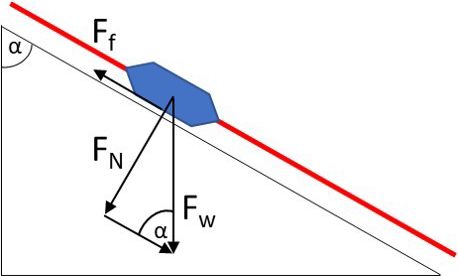
Figure 2. Static friction force Ff and normal force FN applying on long steel piece with a weight of 105 kg. Here, we applied a
a sucker rod contact point (nylon centralizer) as a function of the static friction coefficient for steel on steel of µ = 0.8 (Lee
weight force Fw and the borehole inclination 90◦ −α. and Polycarpou, 2007).
The expected thermal contraction εDTS can also be trans-
lated to a force. Assuming a Young’s modulus for stainless
must consider the friction of their relative motion. This fric- steel of E = 200 GPa (Cardarelli, 2018) and given the cross-
tion would yield a stick–slip motion, which is observed al- sectional area of the rod (Arod = 2.9 cm2 ), we can calculate
most everywhere when two solid objects are moving rela- the applied force Fapp at each location along the rod which
tive to one another. A detailed review of the origins of stick– was thermally induced within the investigated 1 h cold-water
slip behavior in mechanical parts as well as an experimental injection period:
and theoretical analysis on stick–slip characteristics is pre-
sented in the literature (e.g., Berman et al., 1996). In the sim- Fapp = σ · Arod = E · εDTS · Arod . (5)
plest case, a stick–slip motion appears when the static friction
force Ff between two stationary solid bodies is overcome. A For simplicity, we assume that the elasticity from the fiber-
schematic drawing of the forces on an interval of the sucker optic cable and the nylon centralizers are neglectable and that
rod construction at a depth with borehole inclination is pre- the steel dominates the mechanical behavior of the structure.
sented in Fig. 2. Furthermore, we make the assumption that no mechanical
The static friction force Ff can be calculated according to stresses are exerted on the rod prior to the cold-water injec-
tion. This allows us to set a zero-force baseline before injec-
Ff = µ · FN , (3)
tion start for the stick–slip analysis.
where Fn is the normal force and µ the static friction coef-
ficient. The value for µ = 0.36 was obtained from a plate- 2.4 Stick–slip event detection and picking
to-plate experimental analysis on the stick–slip behavior be-
In the DAS data we monitored repeating vibrational events
tween steel and a glass-fiber-reinforced nylon specimen (Mu-
with ongoing cold-water injection in the deeper part of the
raki et al., 2003). The force FN is calculated according to
well. These events are characterized by a sudden DAS am-
FN = Fw · sin α = g · m · sin α, (4) plitude peak at some depth and an up- and downward di-
rected move-out. With time, the spatiotemporal distribution
where Fw is the gravitational weight force and α the bore- of these vibrational events changes. To automate the detec-
hole inclination. Each sucker rod element is 9.1 m long, tion of depth location and move-out of an event, we employ
weights 15.7 kg and is equipped with four nylon centraliz- a short-term/long-term average (STA/LTA) trigger (Allen,
ers and the fiber-optic cable (20 g/m). Therefore, the weight 1978; Vaezi and van der Baan, 2015) using the Python tool-
force for each contact point of the rod construction yields box ObsPy (Beyreuther, et al., 2010). The parameters used
Fw = 9.81 m/s2 · 15.9 kg / 4 = 39.0 N. Regarding the low- for the STA/LTA analysis can be found in Table 2.
ermost part of the rod construction as an example, this
means that for the last nylon centralizer (borehole inclina-
tion of 54◦ ), a static friction force of Ff = 0.36 · 39.0 N · sin 3 Results
(54◦ ) = 11.3 N is calculated. With respect to contraction of
an initially unstressed rod construction, for each subsequent Figure 3 shows examples of raw and unprocessed strain rate
nylon centralizer towards the surface, the friction force of the data measured with the DAS unit in the well at the start of
rod at the given depth is calculated by the cumulative sum of cold-water injection (first subplot), 1 h after start of fluid in-
all friction forces from the nylon centralizers below. The fric- jection (second subplot) and shortly after the end of the 24 h
tion force increases with decreasing well depth. Two further water injection period (third subplot). Each subplot depicts
weights are added to the friction force profile: the bottom end 10 s of data with the same data color scaling. A number of
of the sucker rod is a 1.4 m long steel piece with a weight of features can be recognized in each of the data examples. At
64 kg and the carrier of the pT gauge at 2755 m MD is a 2.2 m the depth marked with the arrow “A”, there is a transition
https://doi.org/10.5194/se-13-161-2022 Solid Earth, 13, 161–176, 2022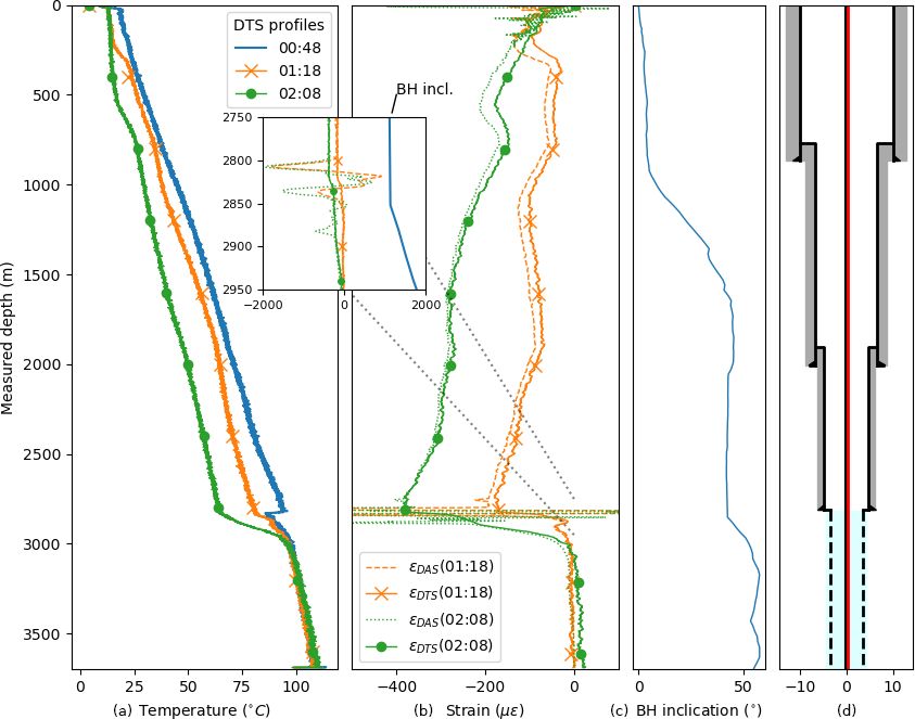
166 M. P. Lipus et al.: Dynamic motion monitoring of a 3.6 km long steel rod in a borehole
from a noisy depth interval above to a rather quiet one be- εDAS . Over this depth interval, the well inclination increases
low. The transition marks the location of the water table in from nearly vertical to 45◦ .
the well. From the wellhead, the water free-falls down to the At the transition to the 7 in. perforated liner at 2810 m MD
water table at about 170 m below surface. In the cased hole (top liner hanger packer) a notably different εDAS pattern is
section down to the depth of the transition to the perforated measured compared to εDTS (box plot in Fig. 4). In the depth
liner, high-velocity tube waves (around 1500 m/s) are present interval 2795–2815 m MD, the expected contraction from
which are reflected at the liner shoe of the 9 5/8 in. casing at εDTS at 01:18 yields −170 µ (−380 µ at 02:08), while the
ca. 2810 m MD (arrow “B” in first subplot). Below B, the ca- estimated contraction from εDAS at 01:18 results in −1740 µ
ble is located inside the perforated liner. The tube waves are (−1950 µ at 02:08) µ between 2805–2810 m MD, which
not further guided in this interval and the noise level is rather is more than a factor 10 higher (factor 5 at 02:08). In
low. In the uppermost 100 m of the perforated liner section the depth interval 2815–2830 m MD, εDAS shows an exten-
(2810–2900 m MD), a strong signal is present in the second sion of the rod with a maximum of 900 µ at 01:18, while
and third subplot (arrow “C”). The arrow “D” marks another εDTS decreases from −160 µ at 2815 m MD to −55 µ at
common characteristic feature in the DAS data which was 2835 m MD. This is the only locations in which the inte-
observed over the analyzed cold-water injection period. This grated strain rate from εDAS shows extension instead of the
abrupt and localized signal is interpreted as a sudden con- predicted contraction. At 2830–2850 m MD, another inter-
traction of the sucker rod. val with extraordinary high εDAS readings relative to εDTS
is present. Below 2850 m MD, εDAS and εDTS again follow
3.1 Sucker rod contraction the same trend at 01:18. At 02:08, the εDAS and εDTS show a
discrepancy down to 2890 m MD and the same trend below.
Figure 4 shows fiber-optic data from DTS and DAS for the The gyro data show a sudden increase in the inclination of
first hour of cold-water fluid injection testing. The first sub- the borehole at 2850 m MD. Between 2900–3100 m MD, the
plot shows three DTS profiles at 00:48, 01:18 and 02:08, temperature difference between the two DTS profiles rapidly
which are −8, +22 and +72 min relative to the cold-water decreases (see Fig. 4, first and second subplot). At 02:08, the
injection start. The entire rod from surface to 3100 m expe- DTS profile shows slightly increased temperatures (+1 ◦ C)
riences cooling. Below the most prominent feed zone of the with a constant offset from 3100 m to the end of the cable
well at 2830 m MD, the cooling of the well decreases. This compared to the DTS profile at 01:18. This leads to a con-
is because most of the injected cold water flows into the for- stant offset of a positive expected strain εDTS . The measured
mation (2825–2835 m MD) and the fluid column below re- strain εDAS shows no offset in this depth interval.
mained rather undisturbed. A theoretical tensile strain from
thermal contraction of the steel rod (and the fiber-optic ca- 3.2 Sudden contraction events
ble) εDTS can be derived from the temperature difference be-
tween the two profiles for a certain depth relative to the pro- 3.2.1 Event description
file at 00:48. The second subplot compares the 15 m moving
average of εDTS calculated after Eq. (1) with the local strain A close-up of raw DAS data is shown for the depth inter-
(εDAS ) calculated after Eq. (2) during the same time interval. val 2500–3300 m MD around the transition from cased hole
The third subplot shows the borehole inclination from the de- to perforated liner 52 min after the start of the cold-water
viation survey. On the fourth subplot, a schematic representa- fluid injection (see Fig. 5). At this time, the DAS records
tion of the casing/liner landing depths is shown together with a transient strain rate anomaly. Similar events are repeatedly
the location of the rod. observed in the course of the measurement during the cold-
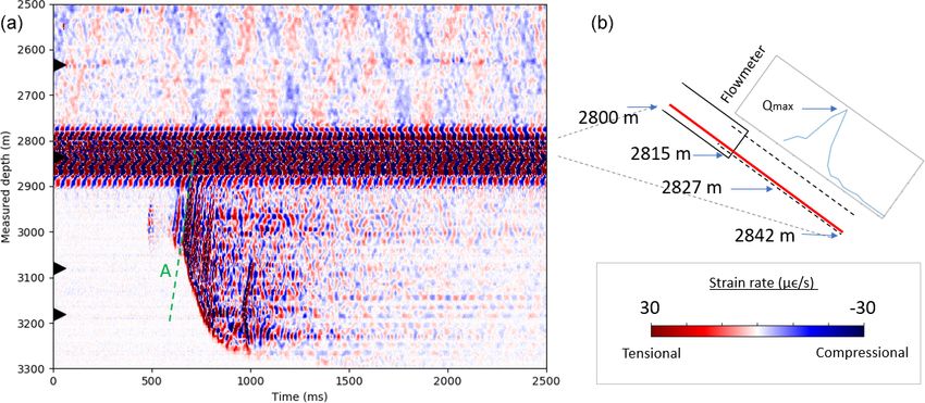
In general, a clear match is visible between εDTS and εDAS water injection periods. Using the event shown in Fig. 5 as
for the entire well which means that the strain the steel rod a representative example, we describe common features of
experiences (εDAS ) follows the predicted thermal contrac- these events in the following. Its origin lies at 600 ms and
tion (εDTS ). However, there are depth intervals where the 3000 m MD and is characterized by an abrupt increase in the
experienced strain (εDAS ) exceeds and others where it falls measured strain rate. The sudden increase in strain rate am-
short on the predicted strain (εDTS ). Until 2825–2835 m MD, plitude propagates both up- and downwards along the well
where the most prominent injection interval is located, 1T with a compressional and tensional sign of amplitude, re-
increases with increasing depth. At the injection interval 1T spectively, where the propagation velocity upwards is ap-
rapidly increases. Below this zone, no thermal contraction is proximately 3900 m/s (green line A in Fig. 5). In contrast,
expected. the downward propagation velocity is slower and shows ir-
Along the 13 3/8 in. casing interval (from top liner regularities from 650–1260 m/s. Most striking is the decay
hanger 13 3/8 in. at 768 m MD to top liner hanger 9 5/8 in. of the velocity from 3200 m MD onwards and the eventual
2010 m MD), εDTS and εDAS are negative and show the same stop of propagation slightly above 3300 m MD. In an upward
trend, thus indicating the expected contraction. In absolute direction, this event is halted somewhere in the noisy inter-
values expected strain εDTS exceeds the measured strain val where the reservoir section of the borehole begins. The
Solid Earth, 13, 161–176, 2022 https://doi.org/10.5194/se-13-161-2022
M. P. Lipus et al.: Dynamic motion monitoring of a 3.6 km long steel rod in a borehole                                                   167

Figure 3. DAS raw data examples over the scope of the cold-water injection phase for (a) the onset of fluid injection, (b) ongoing injection
and (c) termination of fluid injection. Blue colors show relative compression and red colors relative extension. The color ranges are the same
for all subplots.

Figure 4. Downhole monitoring data during the cold-water injection test. (a) DTS temperature profiles. (b) Comparison of strain profiles
εDTS and εDAS . (c) Borehole inclination. (d) Wellbore schematic.

https://doi.org/10.5194/se-13-161-2022                                                                   Solid Earth, 13, 161–176, 2022
168                                  M. P. Lipus et al.: Dynamic motion monitoring of a 3.6 km long steel rod in a borehole

event is followed by elastic reverberations that decay after         (b) the lower end and (c) the upper end of the event accord-
approximately 0.5 s.                                                 ing to the STA/LTA algorithm. Figure 8 shows one example
   Further examples of such events are plotted in Fig. 6             of the automated detection with the STA/LTA trigger. The
(events A, B, C and D). They all have in common that they            upper subplot shows an example trace of raw DAS data at
originate below 2900 m MD and trigger a contraction above            a depth of 3120 m MD (marked by the black arrow in the
and an extension below. The previously discussed event is            lower subplot) and the corresponding STA/LTA characteris-
characterized by a smaller precursor 100 ms before the origin        tic function. Beginning and end of the detection are marked
of the large event at the same depth. Precursors and succes-         by the green and orange crosses, respectively. The lower sub-
sors can also be observed in the examples in Fig. 6 (in par-         plot shows spatiotemporal DAS data and the detection of two
ticular in Fig. 6, event B), yet the events shown here are dis-      vibrational events.
tinguished by the fact that their upwards propagation extends           All vibrational events which occurred within the first
beyond the noisy reservoir section. All exemplary events ex-         72 min of cold-water fluid injection are plotted in Fig. 9.
cept event A, whose downward propagation is arrested rather          Gray circles mark the spatiotemporal origin of vibrational
suddenly, have in common that the up- and downward prop-             events. The corresponding vertical black line indicates the
agation slow down before coming to a halt. Another striking          spatial extent of the respective event. In this representa-
observation in all of the events is that the initial onset propa-    tion, events with a spatial extent of less than 20 m are ne-
gates slower than the reverberations in the coda.                    glected. Such small events occur between 4–10 times per
   While the exact shape of the spatial propagation and length       minute in the depth region from 1250–2750 m MD over the
varies (length between 20–1600 m), the duration of these             entire investigated 72 min after fluid injection start. Within
events is mostly in the range of 0.5 s with some fading              the first 15 min, only a relatively small number of big-
noise/reverberation afterwards. These events typically show          ger vibrational events occur, i.e., events which extend over
a tensional signal at the energy front in the downward direc-        more than 20 m. Early events (within the first 5 min rela-
tion, while the initial energy front upwards is mostly com-          tive to injection start) appear in the depth region between
pressional. As the vibrational signal propagates along the           1250–1900 m MD. Except for two large events (4 min: 2260–
rod, a succession of compressional and tensional waves is            2730 m MD; 6 min: 2040–2700 m MD), the spatial extent of
created which moves with a velocity of about 3900 m/s along          the vibrational events is rather small. One single event was
the rod (as shown by the green line A in Fig. 5). The down-          recorded at a depth of 3540–3580 m MD close to the shoe
ward propagation of the first arrival changes its velocity from      of the installation. With time, the depth of vibrational events
the onset of the event towards the end of the vibrational            increases to 2900 m MD. From 17 min onwards, the occur-
event. In the first 50 ms, it increases in velocity; then it stays   rence of vibrational events is mostly constrained in the depth
constant before it gradually decreases in velocity at around         region from 2900–3100 m MD. The maximum spatial extent
700 ms below 3200 m MD.                                              of large vibrational events increases with time. From 01:18
   The four black arrows on the left y axis in Fig. 5 indi-          (+22 min after injection start) onwards, most of the events
cate the time series for which the four spectrograms shown           extend into the depth region of 2835–3080 m MD. At 02:08
in Fig. 7 were calculated with a moving window of 250 ms.            (+72 min to injection start), the spatial extent of the events is
The DAS strain rate time series at 3000 and 3200 m MD show           2500–3470 m MD.
the onset of the slip event at 0.5 s with dominant frequen-             With time, the frequency of the occurrence of the events
cies of the first break between 30 and 75 Hz. The slip only          decreases: 4–5 h after injection start, large events (such as
lasts approximately 0.5 s, but reverberations of different du-       in Fig. 6c and d) appear every 10–15 min; 8 h after injection
ration and different frequencies can be observed in the band         start, large events appear approximately every 25–40 min.
below 30 Hz depending on the rod segment. For instance,
at 3000 m MD long-lasting reverberations occur at ∼ 10 Hz,           3.3   Friction force model
whereas at 3200 m MD they occur at 20 Hz. As can be seen
from the spectrogram from the DAS strain rate recordings             The static friction force Ff after Eq. (3) is compared to the
at 2700 and 2835 m MD, the slip event does not penetrate             applied force from thermal contraction of the rod Fapp after
into and beyond the feed zone, whose characteristic noise at         Eq. (5), which was evaluated for the period from injection
24 Hz remains undisturbed just as the low-frequency pattern          start to 01:18 (+22 min after start of injection) and to 02:08
of the tube waves above.                                             (+72 min after start of injection) (Fig. 10). The gravitational
                                                                     weight force Fw per nylon centralizer is constant for every
3.2.2   Event detection over time                                    contact point of the rod. The force needed to overcome the
                                                                     cumulative static friction Ff is a function of the borehole in-
We applied a STA/LTA algorithm to automate the detection             clination. Ff increases from the bottom of the rod installation
of the sudden vibrational events within the first 72 min of          at 3691 m MD towards 1000 m MD. The bottom end of the
cold-water fluid injection. Three attributes are obtained for        sucker rod and the carrier of the pT gauge at 2755 m MD
each event: (a) the depth location where the event starts;           create an additional static friction force of 0.4 and 0.5 kN, re-

Solid Earth, 13, 161–176, 2022                                                            https://doi.org/10.5194/se-13-161-2022
M. P. Lipus et al.: Dynamic motion monitoring of a 3.6 km long steel rod in a borehole 169 Figure 5. Sucker rod contraction event displayed by strain rate DAS data (a). The black arrows on the left y axis mark the depth location of time series used for the spectrograms in Fig. 7. Line “A” marks the move-out of the signal at a speed of 4000 m/s. The schematic drawing shows the inclination of the borehole with the fiber-optic cable (red) lying inside of the casing (b). The inflow profile from a wire line flowmeter measurement is shown by the blue graph. Figure 6. Four raw DAS data examples of sucker rod events with the integrated strain rate (εDAS ) over a period of 3 s. The timing of the events relative to the start of cold-water injection is as follows: A – +65 min; B – +110 min; C – +147 min; D – 210 min. spectively. Above 1000 m MD, the well is nearly vertical and close to Ff . This indicates that forces are sufficient to initiate only little static friction is expected. The static friction Ff at relative motion between sucker rod and casing at that depth. 1000 m MD yields 26.1 kN. Fapp at 01:18 is lower than Ff for With ongoing cold-water fluid injection, the applied forces the entire installation length. Only in the depth interval 2731– Fapp increase with further decreasing temperatures. At 02:08, 2820 m MD does Fapp approach a force of 10.5 kN, which is Fapp surpasses the frictional forces in the depth range from https://doi.org/10.5194/se-13-161-2022 Solid Earth, 13, 161–176, 2022
170                                   M. P. Lipus et al.: Dynamic motion monitoring of a 3.6 km long steel rod in a borehole

Figure 7. Spectrograms for a 250 ms moving window at different depth along the well during the sudden vibrational event depicted in Fig. 5.
Red colors indicate high amplitudes, blue colors low amplitudes. The relative amplitudes are displayed by the same color ranges for all
subplots.

Figure 8. STA/LTA trigger algorithm applied as an automated detection method for vibrational events. Trigger start and end is marked with
green and orange crosses.

2150–2912 m MD. Ff and Fapp intersect at 17.0 and 9.3 kN,               4   Discussion
respectively. At the depth interval from 2732–2820 m MD,
the applied force peaks at 22.0 kN (shown in Fig. 10). For              With the help of distributed fiber-optic temperature and
all estimates given above, it is assumed that the sucker rod            acoustic data, we monitored a cold-water injection period
did not move relative to the casing; i.e., thermal stresses can         in a geothermal well at the site Schäftlarnstraße, Munich.
build up but will not be released by relative motion.                   The downhole monitoring data allow for an analysis of the
                                                                        deformation of the 3.6 km long sucker rod/fiber-optic cable
                                                                        construction due to cooling. We observe numerous localized
                                                                        episodes of large strain rates that nucleate along the inclined
                                                                        stretch of the borehole and propagate both towards greater

Solid Earth, 13, 161–176, 2022                                                                https://doi.org/10.5194/se-13-161-2022
M. P. Lipus et al.: Dynamic motion monitoring of a 3.6 km long steel rod in a borehole 171 Figure 9. Gray circles and black vertical lines indicate the spatiotemporal origin and spatial extent of vibrational events in the well, respec- tively. The shown period comprises the first 72 min of cold-water fluid injection. Figure 10. Comparison of static friction Ff with applied forces Fapp from thermal contraction of the rod within the first 72 min of cold-water fluid injection. The pale colors in Fapp originate from measured DTS data, and the solid lines are constructed by a moving average over 15 m. https://doi.org/10.5194/se-13-161-2022 Solid Earth, 13, 161–176, 2022
172                                  M. P. Lipus et al.: Dynamic motion monitoring of a 3.6 km long steel rod in a borehole

depth and the surface. Such events induce quickly declin-           data. Especially from 2800–2900 m MD, constantly high en-
ing elastic vibrations along the entire extent of the affected      ergy is recorded by the system. The second explanation could
interval. The emergence of these vibrational events strongly        be that the integrated DAS data measured a true deformation
correlates with the beginning of the fluid injection. In the fol-   of the construction. In the depth region around 2800 m, the
lowing, we thus argue that the vibrational events are a result      annular space of the borehole is rather irregular (transition
of the substantial temperature changes which the sucker rods        to 7 in. liner interval, localized increase in the borehole incli-
with the optic fiber are exposed to. The contraction of the         nation; see Fig. 4c). The repeating sudden sucker rod events
sucker rods upon cooling induces stress where the sucker rod        might lead to an uneven distribution of the thermal stresses
is held to the borehole wall by frictional forces. On the ba-       along the rod. Interestingly, the most prominent feed zone of
sis of a simple mechanical model we show that accumulated           the well coincides with the one single DAS interval which
stresses may eventually exceed the friction giving rise to sud-     shows an extensional signal.
den stress release and the observed strain changes.                    The sudden slip events presented in this study show some
                                                                    similarity to the slip events which were previously observed
4.1   Assessment of measuring errors                                in FIMT-type fiber-optic installation in a geothermal well
                                                                    (Miller et al., 2018). In the reported DAS campaign, a fiber-
Our monitoring data analysis is based on a debatable ap-            optic cable was installed in a geothermal well, and it is ar-
proach of integrating DAS data over longer time periods. To         gued that repeated thermal cycles led to a loss of frictional
obtain the εDAS profile over the period of 1 h, a total num-        coupling between fiber-optic cable and the borehole wall.
ber of 3.6 million strain rate profiles are integrated (sample      Miller et al. (2018) reported that a sudden loss triggered a
rate: 1000 Hz). Such a numerical operation has a high risk of       movement of the cable with a first arrival speed of 4600 m/s
creating numerical errors due to, e.g., rounding off or value       (we measured a first arrival speed of 4000 m/s). The inte-
truncation. In addition, the smallest systematic error in the       grated strain of the reported event shows a balance towards
DAS measurement system results in a significant drift over          absolute contraction which we also observe in our events.
time which would misrepresent the strain profile measured           Another similarity is given by the frequency content of these
by the sensing fiber. Also, it is well known that for FIMT-type     events. They recorded a dominant frequency of 45 Hz with
installations, the gel filling allows for creep and differential    some harmonics in both directions which we also observed
movement of fibers with respect to its surroundings, which          in our data (see Fig. 7 at 3000 m MD).
makes strain sensing unreliable for greater deformations and
longer periods (e.g., Lipus et al., 2018; Becker et al., 2020).     4.3   Stick–slip rod behavior
However, creep over many meters or even kilometers is most
likely improbable. To strengthen the meaningfulness of our          We calculated the static friction force Ff along the rod con-
integrated strain profile, we analyzed the εDAS for a deeper        struction by a cumulative sum of the friction of each nylon
section of the well, where little temperature change (ca. 1 ◦ C)    centralizer with the borehole inner wall. Independently of
was measured by the DTS. In 3500 m depth, we do not ob-             that, we computed the applied force Fapp on the rod construc-
serve any strain accumulation after temporal integration of         tion by thermal contraction using the DTS monitoring data.
strain rate data over a period of 60 min. This indicates that       By comparing both curves, we can distinguish depth regions
the measured strain rate has no significant drift during the        where the rod remains immobile (Ff > Fapp ) and depth re-
time of interest. For measurements with higher amplitudes           gions where the applied forces overcome the static friction
such as within the depth interval 2800–2900 m, non-linear           force (Ff < Fapp ). The temperature difference in the course
effects influencing the temporal integration of the data can-       of the investigated time period is particularly high over the 9
not be excluded.                                                    5/8 in. liner interval (depth region from 2485–2890 m MD),
                                                                    which in consequence also means that Fapp is high. Accord-
4.2   DAS data integration                                          ing to our model calculation, the contraction forces surpass
                                                                    the frictional forces at 2800 m MD around 01:18 (22 min af-
We integrated DAS data in time over 72 min to assess the            ter injection start). This result implies that after this time,
absolute contraction of the rod construction prior to the cold-     the construction can contract in this depth interval. In other
water injection start (see Fig. 4). For the well interval from      words, the thermal stresses on the rod construction in this
the water table to the transition to the perforated liner, the      depth region are high enough that the rod starts to move and
results show a good match to the contraction that was the-          to contract. Hence, the literature values assumed for the static
oretically assumed from the cooling of the well. However,           friction between sucker rod and steel liner are assumed to ap-
from 2800–2900 m MD, we obtain much higher deformation              proximate the real values.
from the DAS data than what we expected. We cannot give                With ongoing cold-water injection and further cooling of
an unambiguous explanation for that but see two likely rea-         the well, the applied forces Fapp increase. This leads to a
sons for that observation. Firstly, the DAS integration process     continuous growing of the depth interval where Fapp sur-
might result in a drift when integrating high-amplitude DAS         passes the static friction Ff of the rod. The STA/LTA detec-

Solid Earth, 13, 161–176, 2022                                                           https://doi.org/10.5194/se-13-161-2022
M. P. Lipus et al.: Dynamic motion monitoring of a 3.6 km long steel rod in a borehole 173
tions match the predictions of the friction fore model. After 5 Conclusion
a rather quiet initial phase of low-energetic events (before
17 min in Fig. 9) which could be caused by the relaxation The field test at the geothermal site Schäftlarnstraße demon-
of previously accumulated stress anomalies along the sucker strates that simultaneous recording of DTS and DAS data
rods, repeated vibrational events start to concentrate in the can be used for a detailed analysis of the deformation of
region 2800–3100 m MD. As the region with Ff < Fapp in- a sucker-rod-type fiber-optic cable installation in a 3.6 km
creases, the length of the vibrational events increases. From deep well. By comparing the theoretical contraction of the
our friction force model, we would expect vibrational events rod structure from DTS with an estimated contraction from
(more specifically: the contraction part of the movement) at DAS, we can distinguish depth intervals with higher and
02:08 in the depth region 2150–2910 m MD. However, the lower thermal stresses in the material. We introduce a friction
observed events extend from 2500–3500 m MD. Regarding force model which accurately predicts the onset and extent of
the upper limit, we can see in Fig. 10 that there is a signif- sucker rod events releasing accumulated thermal stress. This
icant change in slope for Fapp at 02:08 at 2500 m MD. The is an important finding for DAS monitoring in geothermal
friction force model is based on numerous assumptions (i.e., settings because it shows that localized high-energetic vibra-
static friction coefficient nylon steel, Young’s modulus for tional events must not necessarily be related to microseismic
stainless steel, neglecting fiber-optic cable, stress-free initial events occurring in the rock formation but can originate in
conditions) which might not accurately depict the downhole the subsurface construction and the way in which the fiber-
conditions. This could mean that either the calculated applied optic monitoring equipment is installed in the well. More-
force Fapp is too high and/or the static friction force Ff is too over, the friction force model is useful to predict the data
low. quality for DAS measurement campaigns for deep sucker-
With respect to the lower limit of the vibrational events, rod-type fiber-optic installations. Especially for the record-
we predict the contraction part (Fapp (02:08) Fig. 10) of the ings of weak acoustic signals that are, e.g., induced by fluid
vibrational events down to a depth of 2912 m MD from our movement in the annulus, it is essential to know the poten-
friction force model. However, we record vibrational events tial sources of errors and artifacts in the data. During oper-
down to a depth of 3480 m MD. This discrepancy can partly ations which introduce a temporal temperature gradient, the
be explained by the fact that the model prediction only shows thermo-mechanical response of freely hanging steel parts in
the contraction part of the vibrational event. As seen in the the borehole may introduce stick–slip events that must be dis-
cumulative strain εDAS (see Fig. 6 events A and B), the lowest tinguished from any other relevant seismogenic source. Po-
part of a vibrational event yields extension. The most likely tentially, the vibrational energy from the sucker rod events
reason is that the contraction above results in a pulling of the can also be used to study the formation velocity in the near-
rod from a lower-lying region to compensate for the missing field around the borehole. Furthermore, the large-scale con-
rod length. Therefore, the events can be traced down to a traction along certain sucker rod and fiber intervals must be
greater depth than predicted. considered with respect to the location of the distributed sen-
The constant temperature offset by +1 ◦ C in the DTS pro- sor nodes. Our description also serves as a starting point for a
files from 02:08 (relative to 01:18) in the depth interval from more detailed dynamic description of the observed processes.
3100 m MD to the end of the cable is unlikely to be caused This can be of use to predict the onset and depth interval of
by any fluid movement. While DTS temperature measure- such sucker rod events and to contain their destructive poten-
ments did show a variation, no additional offset was recorded tial in case of too quick a cooling of the construction.
from the measured strain εDAS . This could mean that the rod
builds up thermal extensional stresses without actual move-
ment taking place (εDTS > 0, εDAS = 0). However, we spec- Code and data availability. Python scripts and data are available
ulate that the temperature anomaly is related to the process- upon request to the corresponding author.
ing of the DTS data. DTS temperature was measured in a
double-ended configuration. A temperature profile is created
by overlaying the DTS signal from both directions which are Author contributions. TR and KZo conceptualized, planned and
measured consecutively for both fiber branches. Close to the coordinated the monitoring campaign. MPL, FS, CW, TR and DP
conducted the field measurement. MPL performed the DAS data
folding location (at the bottom of the well), an asymmetry
processing. CMK helped in the interpretation of the DAS data. All
in the temperature reading was observed between both fiber
authors contributed in the interpretation of the results. MPL pre-
branches, which does not seem to be caused by any fluid mo- pared the first draft of the paper with contributions from all authors.
tion. Averaging this difference between both branches led to
a temperature offset. This offset was only visible if strong
temperature changes were observed. Competing interests. At least one of the (co-)authors is a member
of the editorial board of Solid Earth. The peer-review process was
guided by an independent editor, and the authors also have no other
competing interests to declare.
https://doi.org/10.5194/se-13-161-2022 Solid Earth, 13, 161–176, 2022174 M. P. Lipus et al.: Dynamic motion monitoring of a 3.6 km long steel rod in a borehole
Disclaimer. Publisher’s note: Copernicus Publications remains liHertz frequencies, Geophys. Res. Lett., 44, 7295–7302,
neutral with regard to jurisdictional claims in published maps and https://doi.org/10.1002/2017GL073931, 2017.
institutional affiliations. Becker, M. W., Coleman, T. I., and Ciervo, C. C.: Distributed
Acoustic Sensing as a Distributed Hydraulic Sensor in Frac-
tured Bedrock, Water Resour. Res., 56, e2020WR028140,
Special issue statement. This article is part of the special issue https://doi.org/10.1029/2020WR028140, 2020.
“Fibre-optic sensing in Earth sciences”. It is not associated with a Berman, A. D., Ducker, W. A., and Israelachvili, J. N.: Origin and
conference. Charactrization of Different Stick-Slip Friction Mechnanisms,
Langmuir, 12, 4559–4563, https://doi.org/10.1021/la950896z,
1996.
Acknowledgements. This work would not have been possible with- Bruno, M. S., Lao, K., Nicky, O., and Becker, M.: Use of Fiber Op-
out the continuous support from our partners involved in the project. tic Distributed Acoustic Sensing for Measuring Hydraulic Con-
The authors are thankful to Stadtwerke München, owner and oper- nectivity for Geothermal Applications, United States: N. p., Web.
ator of the geothermal site Schäftlarnstraße, for providing access https://doi.org/10.2172/1434494, 2018.
to the well site, their premises and well data. The authors would Bücker, C. and Grosswig, S.: Distributed temperature sensing in the
also like to thank the drilling contractor Daldrup for accessing the oil and gas industry – insights and perspectives, Oil Gas Euro-
site during the drilling and well completion operation. Moreover, pean Magazine, 43, 209–215, https://doi.org/10.19225/171207,
we would like to give credit to our colleagues at Erdwerk GmbH 2017.
and Baker Hughes for the close collaboration and fruitful discus- Cardarelli, F.: Ferrous Metals and Their Alloys, in: Materials
sions. From GFZ, the authors are thankful to Christian Cunow and Handbook, Springer, Cham., https://doi.org/10.1007/978-3-319-
Tobias Raab who supported the field work and acquisition of fiber- 38925-7_2, 2018.
optic data. The authors would like to thank Ryan Schultz and the Chang, H. and Nakata, N.: Investigation of the time-lapse
second anonymous referee for reviewing and improving this paper. changes with the DAS borehole data at the Brady
geothermalfield using deconvolution interferometry, SEG
Technical Program Expanded Abstracts, 3417–3421,
https://doi.org/10.1190/segam2020-3426023.1, 2020.
Financial support. The fiber-optic cable was installed in the
Daley, T. M., Freifeld, B. M., Ajo-Franklin, J., Dou, S., Pevzner, R.,
framework of the Geothermal Alliance Bavaria project, funded
Shulakova, V., Kashikar, S., Miller, D. E., Goetz, J., Henninges,
by the Bavarian Ministry of Economic Affairs, Energy and
J., and Lueth, S.: Field testing of fiber-optic distributed acoustic
Technology. A part of this work was financed by the GeCon-
sensing (DAS) for subsurface seismic monitoring, The Leading
nect project (Geothermal Casing Connections for Axial Stress
Edge, 32, 699, https://doi.org/10.1190/tle32060699.1, 2013.
Mitigation), coordinated by ÍSOR, which is funded through the
Daley, T. M., Miller, D. E., Dodds, K., Cook, P., and Freifeld, B. M.:
ERANET cofund GEOTHERMICA (project no. 731117), from the
Field testing of modular borehole monitoring with simultaneous
European Commission, Technology Development Fund (Iceland),
distributed acoustic sensing and geophone vertical seismic pro-
Bundesministerium für Wirtschaft und Energie aufgrund eines
files at Citronelle, Alabama, Geophys. Prospect., 64, 1318–1334
Beschlusses des Deutschen Bundestages (Germany) and Ministerie
https://doi.org/10.1111/1365-2478.12324, 2016.
van Economische Zaken (the Netherlands).
Engineering ToolBox, Metals and Alloys – Young’s Modulus
of Elasticity, available at: https://www.engineeringtoolbox.com/
The article processing charges for this open-access
young-modulus-d_773.html (last access: June 2020), 2004.
publication were covered by the Helmholtz Centre Potsdam –
Finfer, D. C., Mahue, V., Shatalin, S., Parker, T., and
GFZ German Research Centre for Geosciences.
Farhadiroushan, M.: Borehole Flow Monitoring using a Non-
intrusive Passive Distributed Acoustic Sensing (DAS), Society
of Petroleum Engineers, SPE Annual Technical Conference and
Review statement. This paper was edited by Zack Spica and re- Exhibition 27–29 October 2014, Amsterdam, the Netherlands,
viewed by Ryan Schultz and one anonymous referee. https://doi.org/10.2118/170844-MS, 2014.
Förster, A., Schrötter, J., Merriam, D. F., and Blackwell, D.
D.: Application of optical-fiber temperature logging – an ex-
ample in a sedimentary environment, Geophysics, 62, 1107,
https://doi.org/10.1190/1.1444211, 1997.
References Ghahfarokhi, P. K., Carr, T., Song, L., Shukla, P., and Pankaj,
P.: Seismic Attributes Application for the Distributed Acous-
Allen, R. V.: Automatic earthquake recognition and timing tic Sensing Data for the Marcellus Shale: New Insights to
from single traces, B. Seismol. Soc. Am., 68, 1521–1532, Cross-Stage Flow Communication, Society of Petroleum Engi-
https://doi.org/10.1785/BSSA0680051521, 1978. neers, SPE Hydraulic Fracturing Technology Conference and
Beyreuther, M., Barsch, R., Krischer, L., Megies, T., Behr, Y., and Exhibition 23–25 January 2018 The Woodlands, Texas, USA,
Wassermann, J., ObsPy: A Python Toolbox for Seismology SRL, https://doi.org/10.2118/189888-MS, 2018.
81, 530–533, https://doi.org/10.1785/gssrl.81.3.530, 2010. Götz, J., Lüth, S., Henninges, J., and Reinsch, T.: Vertical seis-
Becker, M. W., Ciervo, C., Cole, M., Coleman, T., and mic profiling using a daisy-chained deployment of fibre-optic
Mondanos, M.: Fracture hydromechanical response mea- cables in four wells simultaneously – Case study at the Ketzin
sured by fiber optic distributed acoustic sensing at mil-
Solid Earth, 13, 161–176, 2022 https://doi.org/10.5194/se-13-161-2022You can also read