Climate-model-informed deep learning of global soil moisture distribution
←
→
Page content transcription
If your browser does not render page correctly, please read the page content below
Geosci. Model Dev., 14, 4429–4441, 2021
https://doi.org/10.5194/gmd-14-4429-2021
© Author(s) 2021. This work is distributed under
the Creative Commons Attribution 4.0 License.

Climate-model-informed deep learning of global soil moisture
distribution
Klaus Klingmüller1 and Jos Lelieveld1,2
1 Max   Planck Institute for Chemistry, Hahn-Meitner-Weg 1, 55128 Mainz, Germany
2 The   Cyprus Institute, P.O. Box 27456, 1645 Nicosia, Cyprus

Correspondence: Klaus Klingmüller (k.klingmueller@mpic.de)

Received: 23 December 2020 – Discussion started: 17 February 2021
Revised: 17 May 2021 – Accepted: 29 May 2021 – Published: 19 July 2021

Abstract. We present a deep neural network (DNN) that pro-        ent physical and chemical processes. The implementations
duces accurate predictions of observed surface soil moisture,     of these algorithms quite often have a source code legacy
applying meteorological data from a climate model. The net-       with a history spanning multiple decades. This creates a de-
work was trained on daily satellite retrievals of soil moisture   pendency on the system type, which may limit progress in
from the European Space Agency (ESA) Climate Change               model studies once the CPU performance increase slows
Initiative (CCI). The predictors precipitation, temperature       down, which has been typical in the recent past. In fact, due
and humidity were simulated with the ECHAM/MESSy at-              to challenges in the continued miniaturisation of semicon-
mospheric chemistry–climate model (EMAC). Our evalua-             ductors, such a slowdown is ongoing, which motivates the
tion shows that predictions of the trained DNN are highly         search for other performance gains (Leiserson et al., 2020).
correlated with the observations, both spatially and tempo-          Progress has been made to accelerate weather, climate and
rally, and free of bias. This offers an alternative for param-    atmospheric–chemistry models with general-purpose graph-
eterisation schemes in climate models, especially in simula-      ics processing units (GPUs) (Yashiro et al., 2016; Alvanos
tions that use but may not focus on soil moisture, which we il-   and Christoudias, 2017; Sun et al., 2018; Fuhrer et al., 2018;
lustrate with the threshold wind speed for mineral dust emis-     Müller et al., 2019), but a wider utilisation is pending. Other
sions. Moreover, the DNN can provide proxies for missing          high-performance computing applications, such as lattice
values in satellite observations to produce realistic, compre-    quantum chromodynamics, which have a typically smaller
hensive and high-resolution global datasets. As the approach      codebase and less legacy code, swiftly exploited the compu-
presented here could be similarly used for other variables and    tational resources of GPUs (Egri et al., 2007; Clark et al.,
observations, the study is a proof of concept for basic but ex-   2010). A discipline that not only uses the full potential of
pedient machine learning techniques in climate modelling,         GPUs but also builds its present success on the advent of
which may motivate additional applications.                       GPU computing is machine learning, specifically deep learn-
                                                                  ing (Krizhevsky et al., 2012). Strong commercial interest has
                                                                  even boosted the development of specialised machine learn-
                                                                  ing hardware and software (e.g. Abadi et al., 2015; Jouppi
1   Introduction                                                  et al., 2017; Markidis et al., 2018). Atmospheric and cli-
                                                                  mate models can benefit from this development by making
For decades global climate and atmospheric chemistry mod-         use of the computational capabilities of the new hardware
els have relied on supercomputers with a traditional clus-        to accelerate existing algorithms (Hatfield et al., 2019) or
ter architecture that utilise many powerful compute nodes         by applying machine learning techniques to complement ex-
in parallel. The individual nodes are typically very potent       isting, physical-process-based and (especially) empirical pa-
by themselves, using general purpose central processing unit      rameterisations (Chevallier et al., 2000).
(CPU) cores with large memory. They are required to serve
the needs of diverse algorithms representing many differ-

Published by Copernicus Publications on behalf of the European Geosciences Union.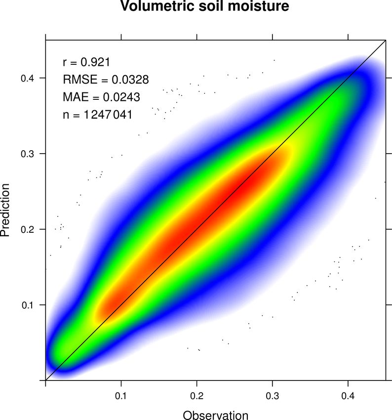
4430                                                K. Klingmüller and J. Lelieveld: Climate-model-informed deep learning

   Given the success of deep learning in many different disci-       This article is structured as follows: the datasets used are
plines (Schmidhuber, 2015; LeCun et al., 2015; Silver et al.,      presented in Sect. 2, the DNN is introduced and evaluated in
2016) it seems likely that atmospheric modelling and cli-          Sect. 3, and applications of the DNN are discussed in Sect. 4
mate science in general can benefit from this methodology          before we draw conclusions in Sect. 5.
(not only in terms of performance gains), and promising re-
sults have been presented lately to this end (e.g. Kadow et al.,
2020; Chandra et al., 2021). However, reservations about ma-       2   Data
chine learning exist. In contrast to physical models, where
                                                                   We used results from a 10-year simulation with the
the simulation result is deduced from the laws of physics and
                                                                   ECHAM/MESSy atmospheric chemistry–climate model
physical parameters, trained models often represent black
                                                                   (EMAC) (Jöckel et al., 2006) version 2.52, covering the years
boxes where the rules by which they compute the output tend
                                                                   2006 to 2015. The exact configuration is described by Kling-
to be non-transparent and cannot easily be modified to repre-
                                                                   müller et al. (2020). Horizontally, the setup employs a Gaus-
sent varied physical conditions. On the other hand, complex
                                                                   sian T63 grid with approximately 1.9◦ spacing. EMAC as-
conventional, phenomenologically derived parameterisations
                                                                   similates observational data by nudging temperature, vor-
at times also lack a clear physical meaning, and their param-
                                                                   ticity and divergence above the boundary layer to meteoro-
eters are often tuned to obtain realistic results, which is es-
                                                                   logical reanalysis data of the European Centre for Medium-
sentially a non-systematic form of training. Moreover, meth-
                                                                   Range Weather Forecasts (ECMWF) and by using the sea
ods for interpreting machine learning models are emerging
                                                                   surface temperature from the same dataset.
(Montavon et al., 2018; Kohoutová et al., 2020). Besides, de-
                                                                      The EMAC output variables we considered are precipita-
pending on the application, it may be irrelevant whether a
                                                                   tion, surface temperature and humidity, which are prepro-
process is implemented as a black box or not if the scientific
                                                                   cessed to daily average values. In addition, we made use
focus is on other processes. For instance, the present study
                                                                   of the static ecosystem rooting depth map of the online
was motivated by the need for reliable soil moisture data to
                                                                   dust emission scheme, originally from Schenk and Jackson
develop a mineral dust emission scheme.
                                                                   (2009).
   Soil moisture near the surface has a significant impact
                                                                      The EMAC data were complemented by daily volumetric
on the emissions of mineral dust (Klingmüller et al., 2016),
                                                                   soil moisture (i.e. the ratio of water relative to soil volume)
and it is generally of great importance for weather and cli-
                                                                   observations from the ESA CCI Soil Moisture Product Re-
mate. It has been identified by the Global Observing Sys-
                                                                   lease v04.5 (Dorigo et al., 2017; Gruber et al., 2017, 2019).
tem for Climate (GCOS) as an essential climate variable
                                                                   This dataset is representative of the soil moisture in the top-
(ECV, Bojinski et al., 2014) and, for example, soil mois-
                                                                   most few centimetres of soil (down to about 5 cm). We used
ture can greatly impact mesoscale convective systems (Klein
                                                                   the dataset that combines retrievals from active and passive
and Taylor, 2020). While detailed parameterisations of soil
                                                                   spaceborne microwave instruments, which we aggregated
moisture exist (e.g. Ekici et al., 2014), many models, such as
                                                                   from the original spatial grid with 0.25◦ spacing to the Gaus-
the ECHAM/MESSy atmospheric chemistry–climate model
                                                                   sian T63 grid of the EMAC results.
(EMAC) (Jöckel et al., 2006), still use relatively simple mod-
                                                                      We subdivided the 10-year period covered by the EMAC
els.
                                                                   simulation into a training period of 8 years from 2006 to 2013
   On the other hand, because moisture at the surface affects
                                                                   and a test period of 2 years from 2014 to 2015. This choice
the dielectric properties of the soil, it can be retrieved well
                                                                   maximises the length of the training period while keeping
remotely using microwaves, and an extensive global daily
                                                                   more than 1 year for testing, allowing the identification of
dataset covering the past 4 decades is provided by the Euro-
                                                                   interannual variations during the testing period. Moreover,
pean Space Agency (ESA) Climate Change Initiative (CCI)
                                                                   using training and testing periods in chronological order, all
(Dorigo et al., 2017; Gruber et al., 2017, 2019).
                                                                   predictions in the testing period represent forecasts. The test
   To make use of the ESA CCI surface soil moisture data
                                                                   period was exclusively used to evaluate the DNN after train-
in climate models, they cannot be imported directly because
                                                                   ing. Every third year of the training period (2008 and 2011)
the daily subsets have substantial gaps depending on the local
                                                                   was used for validating and monitoring the training proce-
retrieval conditions at overpass time. Moreover, merely im-
                                                                   dure.
porting observations would limit model applications to hind-
casting. Therefore, we pursued an alternative approach and
use the satellite data for supervised training of a deep neural    3   DNN model
network (DNN) to predict soil moisture based on modelled
meteorological data. In doing so, we explored the potential        The basic concept of our approach is to relate the observed
of machine learning to complement physical models using            soil moisture to relevant quantities modelled by the global
an introductory example, which demonstrates the useful re-         climate model. We applied a simple DNN architecture which
sults that can be achieved with limited technical effort and       operates on one grid cell at a time. As a consequence, the
which might instigate further applications.                        DNN can easily be integrated as a submodel in global climate

Geosci. Model Dev., 14, 4429–4441, 2021                                            https://doi.org/10.5194/gmd-14-4429-2021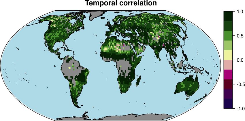
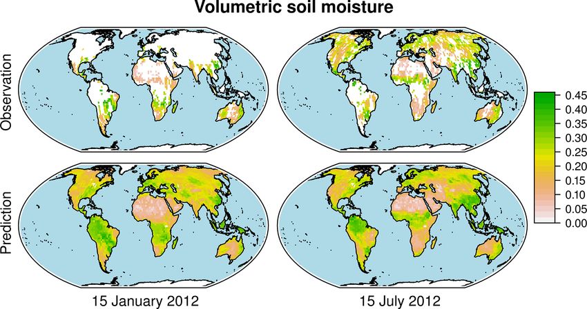
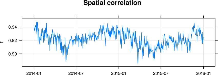
K. Klingmüller and J. Lelieveld: Climate-model-informed deep learning                                                           4431

models such as EMAC. The meteorological variables used as           observations, with a Pearson correlation coefficient of 0.92,
predictors are selected based on their availability in the cli-     and do not show any bias, resulting in a small root-mean-
mate simulation output and physical relevance: the rain rate        square error of 0.033 and a mean absolute error of 0.024,
represents the source of soil moisture, whereas surface tem-        which is an order of magnitude smaller than the average data
perature and atmospheric humidity control soil drying. To           values. Note that the Gaussian grid has more grid cells per
account for cumulative effects, in addition to the actual daily     area at higher latitudes, giving those regions more weight in
mean rain rate, surface temperature and specific humidity, we       this comparison, but the number of relevant grid cells in polar
provided the DNN with the corresponding values lagged by            regions is small.
1 d, the mean of values with 2 to 3 d lag, and the mean of 4           While Fig. 2 combines the effect of the spatial and tempo-
to 7 d lagged values. According to preliminary tests, consid-       ral variability, Fig. 3 shows the spatial correlation for each
ering longer lags did not yield a significant improvement, but      day separately, using all grid cells with observations dur-
it might become relevant if the overall performance can be          ing that day. The correlation coefficient attains high values
enhanced in future versions. To account for regional charac-        around 0.92 throughout the test period and rarely drops be-
teristics such as soil properties, the DNN uses longitude and       low 0.9. Considering that the training takes place before the
latitude, encoded in the triple sin(lon), cos(lon), and sin(lat),   test period, it is noteworthy that there is no significant decline
as well as the local rooting depth. Likewise, to account for        of the correlation over the two years. Essentially, at any time
seasonality, for example due to vegetation variation, we sup-       the DNN yields a realistic representation over the globe, pre-
plied the DNN with the time of year encoded as sin(2π t/a)          dicting low soil moisture in arid regions and high soil mois-
and cos(2π t/a), where t/a is the time in years. In total, this     ture in wet areas.
amounts to 18 input variables that had to be mapped to one             Equally important is a realistic representation of the tem-
output variable, i.e. the surface soil moisture.                    poral variation for each grid cell. Due to the strong temporal
   For the above purpose, we employed a generic DNN of lin-         variability of weather and precipitation in particular, this is
early stacked densely connected layers as illustrated in Fig. 1.    more challenging, and we do not expect equally high corre-
Four hidden layers of 512 units with rectified linear activa-       lation coefficients as those found for the spatial correlation.
tion are followed by the output layer with a single unit and        Nevertheless, Fig. 4 shows that the temporal correlation co-
linear activation. There is no strict formula for the number of     efficients are globally high, with a mean of almost 0.7, which
layers and units per layer, but DNNs that are too small are         appears to be a good performance when compared with state-
not capable of learning complex rules, whereas DNNs that            of-the-art model data (Dorigo et al., 2017). The correlation
are too large are more at risk of overfitting and require more      coefficient is larger than 0.5 in almost all grid cells except
computational resources. Our values are a compromise that           those representing the extremely dry soils of the Sahara, Rub’
is proving to work well, but systematic optimisation could          al Khali, Taklamakan and Gobi deserts. Related to this, a
possibly yield better results. To generalise the DNN and pre-       slight overestimation by the DNN towards the lower end of
vent overfitting during training, we regularised it by applying     the soil moisture range can be identified in Fig. 2. Training
a 10 % dropout rate to the hidden layers (Hinton et al., 2012)      and evaluation of the DNN are challenging in this range be-
and stopped the training process as soon as the validation loss     cause satellite retrievals are both sparse and uncertain (see,
was no longer improving. Before training, all input and out-        e.g. Fig. S1 in the Supplement); therefore, depending on the
put variables were normalised independently to have a mean          application, some additional effort focusing on these regions
of 0 and a standard deviation of 1. Accordingly, before using       might be required. For dust emissions, the soil moisture in
the DNN for predictions, the same transformations had to be         these regions is too low to significantly influence the results,
applied to the input data, and an inverse transformation had        while it is more relevant in semi-arid regions, where obser-
to be applied to the output.                                        vations and predictions are more reliable (Figs. 4 and S2 in
   We implemented the DNN and performed the training and            the Supplement).
inference using the TensorFlow library (Abadi et al., 2015)            Considering the grid cell centred at 49.4◦ N, 7.5◦ E, the
with the Keras interface (Chollet et al., 2015, 2017) for R         upper panel of Fig. 5 exemplifies how closely the predicted
(R Core Team, 2019). The training took about 40 min on an           volumetric soil moisture time series resembles the observa-
Nvidia Tesla V100 GPU accelerator. The much less compu-             tions. There is no bias in the predictions and the seasonal
tationally demanding predictions were evaluated on common           cycle is well represented. Moreover, the short-term varia-
desktop hardware.                                                   tions in the predictions show a clear similarity to those of
   To assess the overall predictive power of the DNN, we            the observations. Both have a comparable amplitude and fre-
compared the volumetric soil moisture calculations with the         quency, and characteristic features in the observed time se-
corresponding observations for all grid cells and days dur-         ries are reproduced by the predictions, e.g. in July 2014, Oc-
ing the test period (2014 to 2015) where retrievals are avail-      tober 2014, December 2014/January 2015 and March 2015
able. Figure 2 shows the scatter of the 1247041 observation–        (Fig. S3 in the Supplement). These features occur irregularly
prediction pairs. It demonstrates the remarkably high qual-         and are not repeated year after year, which demonstrates that
ity of the predictions, which are strongly correlated with the      the DNN did not simply learn one representative climatology

https://doi.org/10.5194/gmd-14-4429-2021                                               Geosci. Model Dev., 14, 4429–4441, 2021
4432                                                    K. Klingmüller and J. Lelieveld: Climate-model-informed deep learning

Figure 1. DNN architecture and hyperparameters. The input variables on the left are processed by four fully connected hidden layers of
512 units each to yield the soil moisture on the right. All four hidden layers use a rectified linear unit function activation and during the
training use a dropout rate of 10 % to avoid overfitting. The output layer with only one unit applies a linear activation function to obtain the
final result. The DNN operates on normalised variables with a standard deviation of 1 and mean of 0.

but instead utilises information from the meteorological data             duced by the DNN (Figs. S6 to S8). Therefore, if climatic
provided by the climate model. We reiterate that the nudged               changes are represented in the meteorological predictors, the
EMAC meteorology is close but not identical to the real at-               DNN soil moisture will respond to theses changes. The re-
mosphere, and hence small deviations are expected.                        sponse might be limited because in the present configuration
   For the realistic representation of the temporal soil mois-            the DNN can substitute meteorological information with the
ture variation in each grid cell, the meteorological predictors           knowledge of season and location. Consequently, for appli-
are essential. The climatological model obtained by train-                cations in long-term climate projections, training and eval-
ing the DNN and omitting the meteorological predictors still              uation on longer timescales and possibly refinements of the
reaches an overall correlation coefficient of close to 0.9, but           DNN architecture are advisable.
the global mean of temporal correlation coefficient drops                    The spatial coordinate predictors are crucial for a realis-
substantially from close to 0.7 to below 0.5 (Fig. S4 in the              tic spatial variation in the soil moisture. They are the pa-
Supplement). In addition to the interannual variations, the               rameters encoding information on a wide range of surface
variability on timescales shorter than 1 month is lost by ig-             properties, including soil and vegetation types, and substan-
noring the meteorology (Fig. S5 in the Supplement). The                   tially improve the DNN. Less relevant are the seasonal pre-
relevance of the individual meteorological predictors for the             dictors, but, if provided, the DNN makes use of them so that
temporal variations differs regionally. For example, in Eu-               the DNN predictions are sensitive to variations in the time
rope the DNN predictions are sensitive to all meteorological              of year (Figs. S6 to S8) and the temporal correlation is im-
predictors, but in arid and semi-arid regions of the Middle               proved (Fig. S4).
East they are not sensitive to reductions in rain (Figs. S6 to
S8 in the Supplement). Here, all variability is inferred from
temperature and humidity. This does not necessarily imply                 4    Applications
rain to be the least important driver of soil moisture variabil-
ity in the region, rather it is the least reliable predictor due to       The DNN operates on a single grid cell at a time and there-
the uncertainty in modelled precipitation.                                fore can easily be incorporated in climate models, for exam-
   The meteorological predictors are also required to make                ple in the submodel core layer of EMAC. This provides real-
the DNN sensitive to climatic changes. Increasing tempera-                istic soil moisture values to other submodels, which can op-
ture or decreasing humidity promotes soil drying, whereas                 tionally replace the current parameterisation of soil hydrol-
increasing rain enhances the soil moisture, which is repro-               ogy. For instance, this could be advantageous for mineral
                                                                          dust emission schemes, which should account for reduced

Geosci. Model Dev., 14, 4429–4441, 2021                                                      https://doi.org/10.5194/gmd-14-4429-2021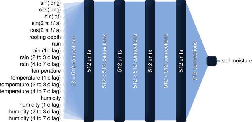
K. Klingmüller and J. Lelieveld: Climate-model-informed deep learning 4433
Mineral dust emissions are predominantly caused by salta-
tion bombardment where saltating particles on impact with
the surface eject finer dust sediments or disintegrate to finer
particles themselves. To activate and sustain a horizontal flux
of saltating particles, the surface friction velocity of the air
has to exceed a threshold that depends on the soil properties.
Soil moisture increases this threshold, thereby reducing the
dust emissions. We studied this effect using the parameteri-
sation presented by Fécan et al. (1999),
u∗t q
2 + 0.17φ 0.68 ,
= 1 + 1.21(w − (0.0014φclay clay )) (1)
u∗td
where u∗t is the threshold surface friction velocity, u∗td is
the corresponding threshold for dry soil, w is the gravi-
metric soil moisture in percent and φclay the soil clay frac-
tion in percent. The equation is applied if the soil moisture
exceeds 0.0014φclay 2 + 0.17φ
clay , representing the minimum
soil moisture required to induce an increase in the thresh-
old. Like Astitha et al. (2012), we combined this soil mois-
ture dependency with the threshold surface friction veloc-
ity parameterisation of Marticorena and Bergametti (1995),
applied to a saltation particle diameter of 60 µm. The full
Figure 2. Comparison of observed and predicted volumetric surface equation for the threshold surface friction velocity is repro-
soil moisture considering all daily grid cell values available globally duced in Appendix A. We evaluated the equation for air
during the years 2014 and 2015. The colours represent the density density ρair = 1.2 kg m−3 using the clay fraction distribution
distribution of the scatter, and outliers are represented by dots. Pear- from Shangguan et al. (2014). To convert the volumetric to
son correlation coefficient r, root-mean-square error (RMSE), mean gravimetric soil moisture we assumed a soil bulk density of
absolute error (MAE) and the number of data points n are provided 1600 kg m−3 . For comparison, we converted the EMAC soil
in the upper-left corner.
water from water volume per area to gravimetric soil mois-
ture using the same bulk density and assuming the water to be
evenly distributed over the soil column defined by the rooting
emissions from wet soils, but so far these have been lim- depth.
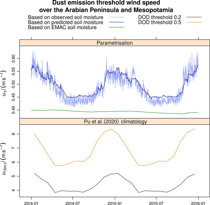
ited by the inadequate representation of soil moisture in the We focused our analysis on Mesopotamia and the Arabian
topmost surface layer by the physically modelled soil water Peninsula, where a significant correlation of soil moisture
(Klingmüller et al., 2018). and dust emissions was reported (Klingmüller et al., 2016),
The lower panel of Fig. 5 shows the time series of the and considered the regional average of the threshold sur-
physically modelled EMAC soil water. Evidently, this time face friction velocity over the territory of Iraq, Israel, Jor-
series is largely unrelated to the observed surface soil mois- dan, Kuwait, Lebanon, Oman, Qatar, Saudi Arabia, the State
ture in the upper panel: the short-term variability is smaller, of Palestine, Syria, the United Arab Emirates and Yemen.
whereas the long-term variability is much larger, showing a The threshold surface friction velocity during the test period
strong decline during summer 2015 that is not present in the is shown in Fig. 6 and was calculated using the observed,
observations. Regardless of the question as to whether this predicted and EMAC-calculated soil moisture. The results
decline reflects a true decline in the water content in deeper based on the observed and predicted soil moisture show good
soil layers or only a model artefact, it is obviously impossible agreement and a strong seasonal cycle. During summer, the
to map the EMAC soil water to a realistic representation of threshold calculated based on the DNN predictions tends to
the observed surface soil moisture in the panel above. How- be slightly higher than that based on the observed values, in-
ever, it is the latter that is required for parameterisations like dicating an effect of the aforementioned challenges in hyper
the mineral dust emission scheme. Because the DNN pre- arid regions. Nevertheless, the difference between both re-
sented here fulfils this requirement, we propose using it as sults is much smaller than the interannual variations, and the
an improvement over the EMAC computed soil water and as DNN result is in the range of the short-term variations in the
a viable alternative to more sophisticated physical soil mois- observation-based results that are due to the varying retrieval
ture models. The algorithm cannot replace physically based coverage. In contrast, the result based on the EMAC soil wa-
soil moisture representations for first-principle process stud- ter has little variability and is therefore inconsistent with the
ies, but it is an accurate substitute for parameterisations that other two results, irrespective of the precise conversion fac-
depend on limited empirical information. tor used to obtain the gravimetric surface soil moisture. We
https://doi.org/10.5194/gmd-14-4429-2021 Geosci. Model Dev., 14, 4429–4441, 2021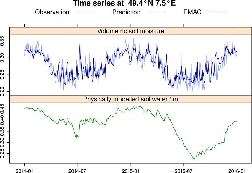
4434                                                    K. Klingmüller and J. Lelieveld: Climate-model-informed deep learning

Figure 3. Spatial correlation of predicted and observed volumetric soil moisture throughout the test period.

Figure 4. Correlation coefficient of the observed and predicted volumetric soil moisture time series in the individual grid cells during the test
years 2014 and 2015. In the grey regions no observations are available during the this period.

conclude that the value of the EMAC soil water, which repre-               speed u10 m,td = 7.5 m s−1 . This value is higher than most of
sents the total water including moisture in deeper soil layers,            the climatological values, however, the latter were derived
is limited in this context, but so far it has been the only esti-          based on 6-hourly wind speeds, whereas the parameterisa-
mate available for EMAC simulations.                                       tion we used is meant for and applied to instantaneous sur-
   Figure 6 additionally shows results from a recent dataset of            face friction velocities that vary on shorter timescales (only
Pu et al. (2020), who have retrieved a climatological monthly              limited by the model time step, e.g. 12 min in our T63 simula-
global distribution of the threshold in terms of the wind speed            tion and even shorter for higher spatial resolutions) and reach
at 10 m altitude based on satellite and reanalysis data. Two               higher peak values. Therefore, the threshold definitions differ
versions of the data represent different assumptions used to               and do not allow direct comparisons of the absolute values.
identify dust events based on the dust optical depth (DOD).                Additionally, because the retrieval of the climatology does
The seasonal cycle is similar to that of the predicted thresh-             not account for dust transport, it may regionally underesti-
old surface friction velocity with a comparable relative am-               mate the threshold.
plitude and a similar but slightly shifted phase. Assuming a                  The substantial variations in the threshold surface friction
logarithmic wind profile, the predicted surface friction ve-               velocity obtained based on the observed soil moisture em-
locity threshold can be converted to the corresponding 10 m                phasise the relevance of soil moisture for dust emissions. The
wind speed u10 m,t = u∗t ln(10 m/z0 )/κ, where κ ≈ 0.4 is the              soil moisture predicted by the DNN is sufficiently realistic to
Von Kármán constant and z0 the surface roughness. Consis-                  reproduce these variations and to account for this important
tent with Astitha et al. (2012), we used the surface rough-                effect in global climate model simulations.
ness z0 = 0.0001 m. According to the logarithmic profile, the                 In addition to the incorporation in global climate models,
threshold that Eq. (A1) yields for dry soils, i.e. the minimal             another application of the DNN is the reprocessing of re-
threshold u∗td = 0.26 m s−1 , corresponds to the 10 m wind                 mote sensing data. Based on meteorological input data, the

Geosci. Model Dev., 14, 4429–4441, 2021                                                      https://doi.org/10.5194/gmd-14-4429-2021
K. Klingmüller and J. Lelieveld: Climate-model-informed deep learning                                                               4435

Figure 5. Time series of the observed and predicted daily volumetric soil moisture values and the EMAC soil water in the grid cell centred
at 49.4◦ N, 7.5◦ E in Europe.

DNN predicts the global daily soil moisture distribution con-          5   Conclusions
sistent with the observations. In contrast to the observational
datasets that have substantial gaps in regions and time pe-
riods where conditions do not allow retrievals, the meteo-             We have presented a machine learning model that relates soil
rological input data does not have any missing values, and             moisture to meteorological conditions. Informed by a climate
consequently the same applies to the predicted soil moisture.          model, this DNN is able to accurately predict satellite-based
The latter can therefore also be used to consistently fill the         surface soil moisture observations, as demonstrated by our
gaps in the observations to obtain a complete daily global             evaluation. Using the example of the threshold wind speed
soil moisture dataset. Figure 7 shows the global distribution          for mineral dust emissions, we showed that the DNN predic-
of the observed and predicted soil moisture on two example             tions can be used for improved representations of processes
days from the training period, one during winter (15 January           depending on the surface soil moisture within climate mod-
2012) and the other during summer (15 July 2012), both in              els.
the Northern Hemisphere. Observations outside the training                The DNN in its present form should be regarded as a proof
period can be processed as well (Fig. S9 in the Supplement),           of concept, and there is room for improvement. The current
but to obtain optimal results the training should include the          DNN architecture, the simple stack of several densely con-
period of interest. Regardless of the extensive regions with-          nected layers, is very generic. While it is generally quite
out observations, the prediction yields global values within a         powerful, it is not tailored to our specific application and
reasonable range, closely resembling the observations where            other concepts might be considered as well. Convolutional
available. Note that in regions or seasons where no or only            neural networks could exploit the spatial relationship of
few observations are available throughout the training pe-             neighbouring grid cells and recurrent neural networks might
riod, the predictions have to be interpreted with caution. This        more optimally account for the causal relationship of the
applies to the rain forests, central deserts and regions per-          soil moisture at successive days including long-term accu-
manently or seasonally frozen or covered by snow. In the               mulative effects. The causal relation is partly addressed in
complete soil moisture distribution the seasonal variations            our implementation by the consideration of lagged meteoro-
become apparent, promoting the DNN predictions for use in              logical variables, representing a temporal convolution. How-
further studies, such as trend analyses. Moreover, in contrast         ever, the prediction is not informed about the conditions prior
to the incomplete observations, the optimised predictions can          to 1 week in the past. This apparently works well for the
straightforwardly be assimilated into climate models.                  surface soil moisture but is probably not sufficient for ad-
                                                                       ditional applications, such as those that require information
                                                                       about the moisture in deeper soil layers. The hyperparame-
                                                                       ters of the DNN, including the number of layers, the num-

https://doi.org/10.5194/gmd-14-4429-2021                                                   Geosci. Model Dev., 14, 4429–4441, 2021
4436 K. Klingmüller and J. Lelieveld: Climate-model-informed deep learning Figure 6. The surface friction velocity threshold above which dust is emitted, averaged over the Arabian Peninsula and Mesopotamia. The surface friction velocity threshold u∗t is computed using the parameterisation provided in the Appendix A. The threshold in terms of the wind speed at 10 m altitude u10 m,t represents the climatological dataset retrieved by Pu et al. (2020). Figure 7. Global distribution of the observed and predicted volumetric soil moisture on a Northern Hemisphere winter (15 January 2012) and summer (15 July 2012) day in the training period. Geosci. Model Dev., 14, 4429–4441, 2021 https://doi.org/10.5194/gmd-14-4429-2021
K. Klingmüller and J. Lelieveld: Climate-model-informed deep learning                                     4437

ber of units per layer and the selection of input variables,
are chosen to be appropriate for the problem but have not
been systematically optimised. We conclude that there are
various pathways for future developments that may enhance
the DNN performance. Nevertheless, the present DNN setup
can already be beneficial for applications such as online min-
eral dust emission schemes in climate models. Therefore, the
trained DNN will be implemented as an EMAC submodel
using the MESSy interface.
   The CPU time required for the inferencing using the
trained DNN is negligible compared to the total computa-
tional demand of a global climate model. Other applications
of DNNs within climate models may be more demanding,
in particular if they process three-dimensional data instead
of only two-dimensional surface data and if they have to be
called more often than once per day. In this case, GPUs or
specialised inferencing hardware can be employed to eval-
uate the trained model, which by design efficiently utilises
such accelerators. In this way, climate models can benefit
from GPUs that are available in many supercomputers with-
out the need for porting complex algorithms to GPUs, and
from the rapid development of machine learning hardware.
   For hindcasting applications, an alternative to implement-
ing the trained soil moisture DNN into climate models is to
import the consistent and comprehensive global soil moisture
prediction from the DNN at runtime. Because such a dataset
is also of general use, it appears to be promising to repeat the
procedure presented here with high-resolution meteorologi-
cal reanalysis data.
   Overall, our example demonstrates that machine learning
models informed by data from traditional, physical-process-
based climate models can perform well in learning and
predicting observational data. In return, they can comple-
ment process parameterisations in climate models, especially
when the parameterisations rely on limited empirical data.
Furthermore, they may help climate models to efficiently
utilise recent hardware architectures.

https://doi.org/10.5194/gmd-14-4429-2021                                Geosci. Model Dev., 14, 4429–4441, 2021
4438 K. Klingmüller and J. Lelieveld: Climate-model-informed deep learning
Appendix A: Surface friction velocity threshold for dust
emissions
The full equation for the threshold surface friction velocity
u∗t used in Sect. 4 is as follows:
v
u
u Dp √ −2
!
0.006 g cm s
u∗t = 0.129t ρp g + 5/2
ρair Dp
1
(
√ B < 10
× 1.928B 0.092 −1
(1 − 0.0858e−0.0617(B−10) ) B ≥ 10
−1
ln zzoso
1 −
×
0.8
10 cm
ln 0.35 zos
v
1 + 1.21max
u
u
×t 0.68 .
2 + 0.17φ
· 0, w − (0.0014φclay clay )
(A1)
The key to Eq. (A1) is as follows.
Dp = 60 µm saltation particle diameter
ρair air density
ρp = 2.65 g cm−3 particle density
g = 9.80665 m s−2 gravitational acceleration
u D
B = ∗tv p friction Reynolds number,
initially B = 1331(Dp /cm)1.56
+ 0.38
−4
v = 0.157 × 10 m s 2 −1 kinematic viscosity of air
zo = 0.01 cm surface roughness length
zos = 0.00333 cm local roughness length of the
uncovered surface
w gravimetric soil moisture in %
φclay clay fraction in %
Geosci. Model Dev., 14, 4429–4441, 2021 https://doi.org/10.5194/gmd-14-4429-2021K. Klingmüller and J. Lelieveld: Climate-model-informed deep learning 4439
Code and data availability. The ECHAM climate model is Scale Machine Learning on Heterogeneous Systems, available at:
available to the scientific community under the MPI-M Software https://www.tensorflow.org/ (last access: 14 July 2021), software
License Agreement (https://mpimet.mpg.de/en/science/modeling- available from tensorflow.org, 2015.
with-icon/code-availability, last access: 11 November 2020, Alvanos, M. and Christoudias, T.: GPU-accelerated atmospheric
MPI-M, 2020). The Modular Earth Submodel System (MESSy) chemical kinetics in the ECHAM/MESSy (EMAC) Earth sys-
is continuously further developed and applied by a consor- tem model (version 2.52), Geosci. Model Dev., 10, 3679–3693,
tium of institutions. The usage of MESSy and access to the https://doi.org/10.5194/gmd-10-3679-2017, 2017.
source code are licensed to all affiliates of institutions that are Astitha, M., Lelieveld, J., Abdel Kader, M., Pozzer, A., and de
members of the MESSy Consortium. Institutions can become Meij, A.: Parameterization of dust emissions in the global at-
a member of the MESSy Consortium by signing the MESSy mospheric chemistry-climate model EMAC: impact of nudg-
Memorandum of Understanding. More information can be ing and soil properties, Atmos. Chem. Phys., 12, 11057–11083,
found on the MESSy Consortium Website (https://www.messy- https://doi.org/10.5194/acp-12-11057-2012, 2012.
interface.org, last access: 11 November 2020, MESSy, 2020). Bojinski, S., Verstraete, M., Peterson, T. C., Richter, C., Simmons,
The data and DNN parameters used in this study are available at A., and Zemp, M.: The Concept of Essential Climate Variables in
https://edmond.mpdl.mpg.de/imeji/collection/eLt_AnQ98XFaaznl Support of Climate Research, Applications, and Policy, B. Am.
(last access: 22 June 2021) (Klingmüller, 2021). Meteorol. Soc., 95, 1431–1443, https://doi.org/10.1175/BAMS-
D-13-00047.1, 2014.
Chandra, R., Cripps, S., Butterworth, N., and Muller, R. D.: Pre-
Supplement. The supplement related to this article is available on- cipitation reconstruction from climate-sensitive lithologies us-
line at: https://doi.org/10.5194/gmd-14-4429-2021-supplement. ing Bayesian machine learning, Environ. Modell. Softw., 139,
105002, https://doi.org/10.1016/j.envsoft.2021.105002, 2021.
Chevallier, F., Morcrette, J.-J., Chéruy, F., and Scott, N. A.: Use of
Author contributions. KK conceived the study, implemented the a neural-network-based long-wave radiative-transfer scheme in
DNN and, supported by JL, wrote the manuscript. Both authors dis- the ECMWF atmospheric model, Q. J. Roy. Meteor. Soc., 126,
cussed the results and finalised the article. 761–776, https://doi.org/10.1002/qj.49712656318, 2000.
Chollet, F., Allaire, J., et al.: R Interface to Keras, available at: https:
//github.com/rstudio/keras (last access: 14 July 2021), GitHub,
2017.
Competing interests. The authors declare that they have no conflict
Chollet, F., et al.: Keras, available at: https://keras.io (last access:
of interest.
14 July 2021), keras.io, 2015.
Clark, M., Babich, R., Barros, K., Brower, R., and Rebbi, C.: Solv-
ing lattice QCD systems of equations using mixed precision
Disclaimer. Publisher’s note: Copernicus Publications remains solvers on GPUs, Comput. Phys. Commun., 181, 1517–1528,
neutral with regard to jurisdictional claims in published maps and https://doi.org/10.1016/j.cpc.2010.05.002, 2010.
institutional affiliations. Dorigo, W., Wagner, W., Albergel, C., Albrecht, F., Balsamo, G.,
Brocca, L., Chung, D., Ertl, M., Forkel, M., Gruber, A., Haas, E.,
Hamer, P. D., Hirschi, M., Ikonen, J., de Jeu, R., Kidd, R., La-
Acknowledgements. We acknowledge financial support from the hoz, W., Liu, Y. Y., Miralles, D., Mistelbauer, T., Nicolai-Shaw,
MaxWater Initiative of the Max Planck Society. N., Parinussa, R., Pratola, C., Reimer, C., van der Schalie, R.,
Seneviratne, S. I., Smolander, T., and Lecomte, P.: ESA CCI Soil
Moisture for improved Earth system understanding: State-of-the
Financial support. The article processing charges for this open- art and future directions, Remote Sens. Environ., 203, 185–215,
access publication were covered by the Max Planck Society. https://doi.org/10.1016/j.rse.2017.07.001, Earth Observation of
Essential Climate Variables, 2017.
Egri, G. I., Fodor, Z., Hoelbling, C., Katz, S. D., Nógrádi, D., and
Review statement. This paper was edited by Rohitash Chandra and Szabó, K. K.: Lattice QCD as a video game, Comput. Phys. Com-
reviewed by three anonymous referees. mun., 177, 631–639, https://doi.org/10.1016/j.cpc.2007.06.005,
2007.
Ekici, A., Beer, C., Hagemann, S., Boike, J., Langer, M., and Hauck,
C.: Simulating high-latitude permafrost regions by the JSBACH
References terrestrial ecosystem model, Geosci. Model Dev., 7, 631–647,
https://doi.org/10.5194/gmd-7-631-2014, 2014.
Abadi, M., Agarwal, A., Barham, P., Brevdo, E., Chen, Z., Citro, Fuhrer, O., Chadha, T., Hoefler, T., Kwasniewski, G., Lapil-
C., Corrado, G. S., Davis, A., Dean, J., Devin, M., Ghemawat, S., lonne, X., Leutwyler, D., Lüthi, D., Osuna, C., Schär, C.,
Goodfellow, I., Harp, A., Irving, G., Isard, M., Jia, Y., Jozefow- Schulthess, T. C., and Vogt, H.: Near-global climate simula-
icz, R., Kaiser, L., Kudlur, M., Levenberg, J., Mané, D., Monga, tion at 1 km resolution: establishing a performance baseline on
R., Moore, S., Murray, D., Olah, C., Schuster, M., Shlens, J., 4888 GPUs with COSMO 5.0, Geosci. Model Dev., 11, 1665–
Steiner, B., Sutskever, I., Talwar, K., Tucker, P., Vanhoucke, 1681, https://doi.org/10.5194/gmd-11-1665-2018, 2018.
V., Vasudevan, V., Viégas, F., Vinyals, O., Warden, P., Watten-
berg, M., Wicke, M., Yu, Y., and Zheng, X.: TensorFlow: Large-
https://doi.org/10.5194/gmd-14-4429-2021 Geosci. Model Dev., 14, 4429–4441, 20214440 K. Klingmüller and J. Lelieveld: Climate-model-informed deep learning Fécan, F., Marticorena, B., and Bergametti, G.: Parametrization of Klingmüller, K., Pozzer, A., Metzger, S., Stenchikov, G. the increase of the aeolian erosion threshold wind friction veloc- L., and Lelieveld, J.: Aerosol optical depth trend over ity due to soil moisture for arid and semi-arid areas, Ann. Geo- the Middle East, Atmos. Chem. Phys., 16, 5063–5073, phys., 17, 149–157, https://doi.org/10.1007/s00585-999-0149-7, https://doi.org/10.5194/acp-16-5063-2016, 2016. 1999. Klingmüller, K., Metzger, S., Abdelkader, M., Karydis, V. A., Gruber, A., Dorigo, W. A., Crow, W., and Wagner, W.: Triple Stenchikov, G. L., Pozzer, A., and Lelieveld, J.: Revised min- Collocation-Based Merging of Satellite Soil Moisture Retrievals, eral dust emissions in the atmospheric chemistry–climate model IEEE T. Geosci. Remote, 55, 6780–6792, 2017. EMAC (MESSy 2.52 DU_Astitha1 KKDU2017 patch), Geosci. Gruber, A., Scanlon, T., van der Schalie, R., Wagner, W., and Model Dev., 11, 989–1008, https://doi.org/10.5194/gmd-11-989- Dorigo, W.: Evolution of the ESA CCI Soil Moisture climate 2018, 2018. data records and their underlying merging methodology, Earth Klingmüller, K., Karydis, V. A., Bacer, S., Stenchikov, G. L., Syst. Sci. Data, 11, 717–739, https://doi.org/10.5194/essd-11- and Lelieveld, J.: Weaker cooling by aerosols due to dust– 717-2019, 2019. pollution interactions, Atmos. Chem. Phys., 20, 15285–15295, Hatfield, S., Chantry, M., Düben, P., and Palmer, T.: Accelerat- https://doi.org/10.5194/acp-20-15285-2020, 2020. ing High-Resolution Weather Models with Deep-Learning Hard- Kohoutová, L., Heo, J., Cha, S., Lee, S., Moon, T., Wager, T. D., ware, in: Proceedings of the Platform for Advanced Scien- and Woo, C.-W.: Toward a unified framework for interpret- tific Computing Conference, PASC ’19, Association for Com- ing machine-learning models in neuroimaging, Nat. Protoc., 15, puting Machinery, New York, NY, USA, 12–14 June 2019, 1399–1435, https://doi.org/10.1038/s41596-019-0289-5, 2020. https://doi.org/10.1145/3324989.3325711, 2019. Krizhevsky, A., Sutskever, I., and Hinton, G. E.: ImageNet Hinton, G. E., Srivastava, N., Krizhevsky, A., Sutskever, I., and Classification with Deep Convolutional Neural Networks, in: Salakhutdinov, R.: Improving neural networks by preventing Advances in Neural Information Processing Systems, edited co-adaptation of feature detectors, CoRR, arXiv [preprint], by: Pereira, F., Burges, C. J. C., Bottou, L., and Wein- 1207.0580, 2012. berger, K. Q., vol. 25, pp. 1097–1105, Curran Associates, Jöckel, P., Tost, H., Pozzer, A., Brühl, C., Buchholz, J., Ganzeveld, Inc., available at: https://proceedings.neurips.cc/paper/2012/file/ L., Hoor, P., Kerkweg, A., Lawrence, M. G., Sander, R., Steil, c399862d3b9d6b76c8436e924a68c45b-Paper.pdf (last access: B., Stiller, G., Tanarhte, M., Taraborrelli, D., van Aardenne, J., 14 July 2021), 2012. and Lelieveld, J.: The atmospheric chemistry general circulation LeCun, Y., Bengio, Y., and Hinton, G.: Deep learning, Nature, 521, model ECHAM5/MESSy1: consistent simulation of ozone from 436–444, https://doi.org/10.1038/nature14539, 2015. the surface to the mesosphere, Atmos. Chem. Phys., 6, 5067– Leiserson, C. E., Thompson, N. C., Emer, J. S., Kuszmaul, 5104, https://doi.org/10.5194/acp-6-5067-2006, 2006. B. C., Lampson, B. W., Sanchez, D., and Schardl, T. B.: Jouppi, N. P., Young, C., Patil, N., Patterson, D., Agrawal, G., Ba- There’s plenty of room at the Top: What will drive com- jwa, R., Bates, S., Bhatia, S., Boden, N., Borchers, A., Boyle, puter performance after Moore’s law?, Science, 368, eaam9744, R., Cantin, P.-l., Chao, C., Clark, C., Coriell, J., Daley, M., https://doi.org/10.1126/science.aam9744, 2020. Dau, M., Dean, J., Gelb, B., Ghaemmaghami, T. V., Gottipati, Markidis, S., Chien, S. W. D., Laure, E., Peng, I. B., R., Gulland, W., Hagmann, R., Ho, C. R., Hogberg, D., Hu, and Vetter, J. S.: NVIDIA Tensor Core Programmabil- J., Hundt, R., Hurt, D., Ibarz, J., Jaffey, A., Jaworski, A., Ka- ity, Performance Precision, in: 2018 IEEE International plan, A., Khaitan, H., Killebrew, D., Koch, A., Kumar, N., Lacy, Parallel and Distributed Processing Symposium Workshops S., Laudon, J., Law, J., Le, D., Leary, C., Liu, Z., Lucke, K., (IPDPSW), 21–25 May 2018, Vancouver, Canada, pp. 522–531, Lundin, A., MacKean, G., Maggiore, A., Mahony, M., Miller, https://doi.org/10.1109/IPDPSW.2018.00091, 2018. K., Nagarajan, R., Narayanaswami, R., Ni, R., Nix, K., Norrie, Marticorena, B. and Bergametti, G.: Modeling the atmospheric T., Omernick, M., Penukonda, N., Phelps, A., Ross, J., Ross, dust cycle: 1. Design of a soil-derived dust emission scheme, J. M., Salek, A., Samadiani, E., Severn, C., Sizikov, G., Snel- Geophys. Res., 100, 16415, https://doi.org/10.1029/95JD00690, ham, M., Souter, J., Steinberg, D., Swing, A., Tan, M., Thor- 1995. son, G., Tian, B., Toma, H., Tuttle, E., Vasudevan, V., Wal- MESSy: The Modular Earth Submodel System, available at: https: ter, R., Wang, W., Wilcox, E., and Yoon, D. H.: In-Datacenter //www.messy-interface.org (last access: 11 November 2020), Performance Analysis of a Tensor Processing Unit, in: ISCA MESSy Consortium, 2020. ’17: The 44th Annual International Symposium on Computer Montavon, G., Samek, W., and Müller, K.-R.: Methods for interpret- Architecture, ACM, New York, NY, USA, 24–28 June 2017, ing and understanding deep neural networks, Digit. Signal Pro- https://doi.org/10.1145/3079856.3080246, 2017. cess., 73, 1–15, https://doi.org/10.1016/j.dsp.2017.10.011, 2018. Kadow, C., Hall, D. M., and Ulbrich, U.: Artificial intelligence re- MPI-M: Code availability, available at: https://mpimet.mpg. constructs missing climate information, Nat. Geosci., 13, 408– de/en/science/modeling-with-icon/code-availability (last access: 413, https://doi.org/10.1038/s41561-020-0582-5, 2020. 11 November 2020), Max Planck Institute for Meteorology, Klein, C. and Taylor, C. M.: Dry soils can intensify mesoscale con- 2020. vective systems, P. Natl. Acad. Sci. USA, 117, 21132–21137, Müller, A., Deconinck, W., Kühnlein, C., Mengaldo, G., Lange, https://doi.org/10.1073/pnas.2007998117, 2020. M., Wedi, N., Bauer, P., Smolarkiewicz, P. K., Diamantakis, Klingmüller, K.: Climate model-informed deep learning of global M., Lock, S.-J., Hamrud, M., Saarinen, S., Mozdzynski, G., soil moisture distribution – data, available at: https://edmond. Thiemert, D., Glinton, M., Bénard, P., Voitus, F., Colavolpe, mpdl.mpg.de/imeji/collection/eLt_AnQ98XFaaznl (last access: C., Marguinaud, P., Zheng, Y., Van Bever, J., Degrauwe, D., 22 June 2021), Max Planck Society, 2021. Smet, G., Termonia, P., Nielsen, K. P., Sass, B. H., Poulsen, J. Geosci. Model Dev., 14, 4429–4441, 2021 https://doi.org/10.5194/gmd-14-4429-2021
K. Klingmüller and J. Lelieveld: Climate-model-informed deep learning                                                                 4441

  W., Berg, P., Osuna, C., Fuhrer, O., Clement, V., Baldauf, M.,       Shangguan, W., Dai, Y., Duan, Q., Liu, B., and Yuan, H.: A global
  Gillard, M., Szmelter, J., O’Brien, E., McKinstry, A., Robin-           soil data set for earth system modeling, J. Adv. Model. Earth Sy.,
  son, O., Shukla, P., Lysaght, M., Kulczewski, M., Ciznicki, M.,         6, 249–263, https://doi.org/10.1002/2013MS000293, 2014.
  Pia̧tek, W., Ciesielski, S., Błażewicz, M., Kurowski, K., Procyk,   Silver, D., Huang, A., Maddison, C. J., Guez, A., Sifre, L., van den
  M., Spychala, P., Bosak, B., Piotrowski, Z. P., Wyszogrodzki, A.,       Driessche, G., Schrittwieser, J., Antonoglou, I., Panneershelvam,
  Raffin, E., Mazauric, C., Guibert, D., Douriez, L., Vigouroux,          V., Lanctot, M., Dieleman, S., Grewe, D., Nham, J., Kalchbren-
  X., Gray, A., Messmer, P., Macfaden, A. J., and New, N.: The ES-        ner, N., Sutskever, I., Lillicrap, T., Leach, M., Kavukcuoglu, K.,
  CAPE project: Energy-efficient Scalable Algorithms for Weather          Graepel, T., and Hassabis, D.: Mastering the game of Go with
  Prediction at Exascale, Geosci. Model Dev., 12, 4425–4441,              deep neural networks and tree search, Nature, 529, 484–489,
  https://doi.org/10.5194/gmd-12-4425-2019, 2019.                         https://doi.org/10.1038/nature16961, 2016.
Pu, B., Ginoux, P., Guo, H., Hsu, N. C., Kimball, J., Marti-           Sun, J., Fu, J. S., Drake, J. B., Zhu, Q., Haidar, A.,
  corena, B., Malyshev, S., Naik, V., O’Neill, N. T., Pérez García-       Gates, M., Tomov, S., and Dongarra, J.: Computational
  Pando, C., Paireau, J., Prospero, J. M., Shevliakova, E., and           Benefit of GPU Optimization for the Atmospheric Chem-
  Zhao, M.: Retrieving the global distribution of the threshold           istry Modeling, J. Adv. Model. Earth Sy., 10, 1952–1969,
  of wind erosion from satellite data and implementing it into            https://doi.org/10.1029/2018MS001276, 2018.
  the Geophysical Fluid Dynamics Laboratory land–atmosphere            Yashiro, H., Terai, M., Yoshida, R., Iga, S.-I., Minami, K.,
  model (GFDL AM4.0/LM4.0), Atmos. Chem. Phys., 20, 55–81,                and Tomita, H.: Performance Analysis and Optimization of
  https://doi.org/10.5194/acp-20-55-2020, 2020.                           Nonhydrostatic ICosahedral Atmospheric Model (NICAM)
R Core Team: R: A Language and Environment for Statistical                on the K Computer and TSUBAME2.5, in: Proceedings
  Computing, R Foundation for Statistical Computing, Vienna,              of the Platform for Advanced Scientific Computing Confer-
  Austria, available at: https://www.R-project.org/ (last access:         ence, PASC ’16, Association for Computing Machinery, New
  14 July 2021), 2019.                                                    York, NY, USA, 8–10 June 2016, Lausanne, Switzerland,
Schenk, H. J. and Jackson, R. B.: ISLSCP II Ecosystem                     https://doi.org/10.1145/2929908.2929911, 2016.
  Rooting Depths, ORNL Distributed Active Archive Center,
  https://doi.org/10.3334/ORNLDAAC/929, 2009.
Schmidhuber, J.: Deep learning in neural networks:
  An       overview,      Neural      Networks,     61,     85–117,
  https://doi.org/10.1016/j.neunet.2014.09.003, 2015.

https://doi.org/10.5194/gmd-14-4429-2021                                                   Geosci. Model Dev., 14, 4429–4441, 2021
You can also read