Contracting alignment patterns of mixed composition UHECRs nuclei deflected in the galactic magnetic field - Indico@KIT (Indico)
←
→
Page content transcription
If your browser does not render page correctly, please read the page content below
Contracting alignment patterns of
         mixed composition UHECRs nuclei
       deflected in the galactic magnetic field

               Correct GMF   +30° wrong
    -30° wrong  knowledge

Marcus Wirtz, HAP Workshop 2019, 19.02.2019
Motivation – Search for point source patterns
                                                                                source
    ✗ Discovery of a significant energy ordering,
      would be a discovery of the sources
    ✗ Including charge in “multiplet analysis”
      would lead to exploding combinatorics

                                                                                         arrival

                      All p-values
                      above 6%
                                                                                    outside galaxy

                                                    (charge sensitive observable)

2    Marcus Wirtz
                                                                                    outside galaxy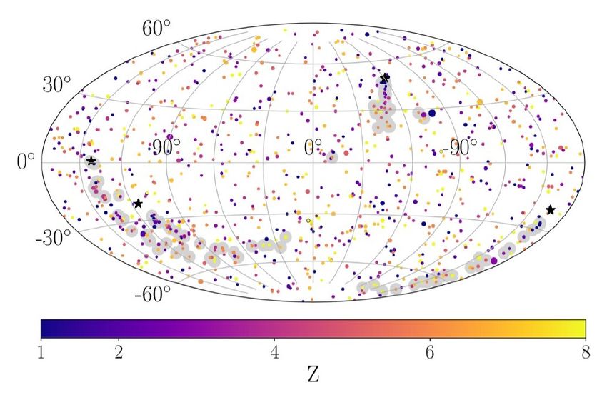
Overview

    I. Contracting alignment patterns: Simultaneous fit to all cosmic ray charges
      (~1000) with Tensorflow, to contract alignment patterns given a galactic
      magnetic field model
     (M. Erdmann, L. Geiger, D. Schmidt, M. Urban, M. Wirtz, Astroparticle Physics, 108, 74-83, 2019)

    II. Compass method: Multi dimensional fit to the galactic magnetic field using
      strongest occurrences of UHECR aligments

3     Marcus Wirtz
Contracting alignment patterns
Fit Concept
      ✗ Contracting mixed composition multiplets by a fit to all charges and “source
         positions” with a suitable loss term and a galactic mangnetic field model

    “charge”
    “source”

           “Fit parameter”           “Transformation”       “Observed direction”

                                                                                     Minimizing loss by
      ✗ Defining loss term:                                                          backpropagation
                                                                                         technique

                   “Distance loss”                      “Cluster loss”                    “Charge loss”

               Keeps arrival directions          Clusters source positions          Keeps charges compatibel
                                             in as few directions as possible      with their energy and shower
                                                (preferred along GMF axis)               depth information
4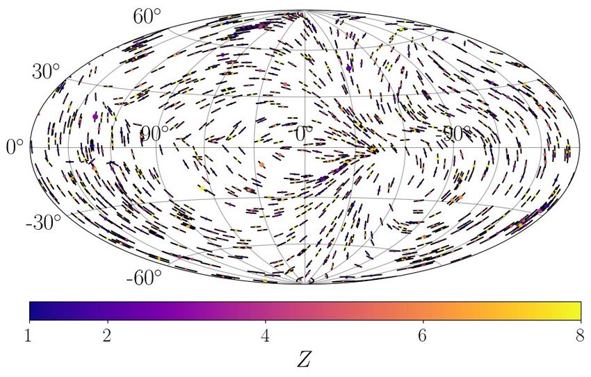
Loss terms
                                                   Three components drive the fit

     Distance loss (arrival directions within uncertainties)

    Entropy like cluster loss (minimize “potential energy”)

                          “Elliptical fisher distribution”

     Compatibility with shower depth distribution

5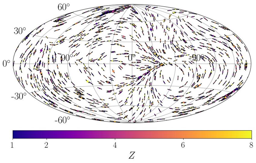
Scenario for realistic deflection model

    ✗   Cosmic rays follow AUGER
        energy spectrum, E > 40 EeV
    ✗   Charge uniform up to CNO
        group (Z = 1 … 8)
    ✗   4 sources each emitting 25
        CRs + 900 background CRs
    ✗   Deflection model:
        JF12 galactic field model
        + rigidity dependent smearing

                                        How to transport gradients over an
                                        arbitrary galactic field transformation?
6       Marcus Wirtz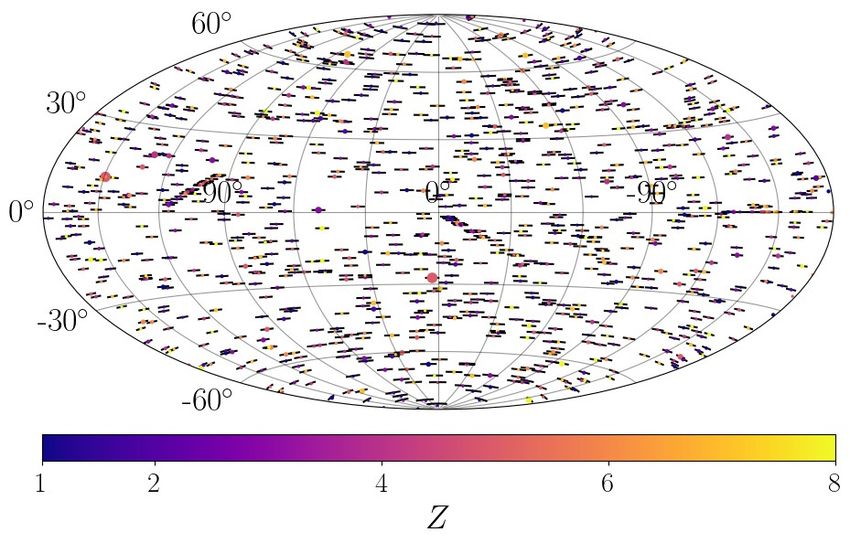
MagNet – Deep neural network for GMF transformation
    ✗ The transformation of directions outside our galaxy to observed directions
      is not differentiable (depends on magnetic field model)

                          backprop.

7    Marcus Wirtz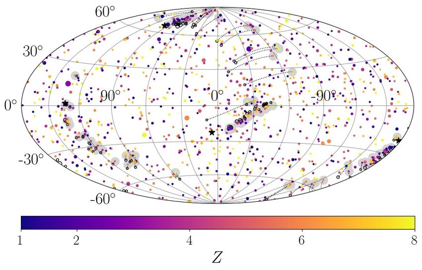
MagNet – Deep neural network for GMF transformation
    ✗ The transformation of directions outside our galaxy to observed directions
      is not differentiable (depends on magnetic field model)

                          backprop.
                                               Network is able to interpolate between
                                                simulated spatial points and rigidities

    ✗ Deep neural network learns
      (5 layers, 100 nodes):

7    Marcus Wirtz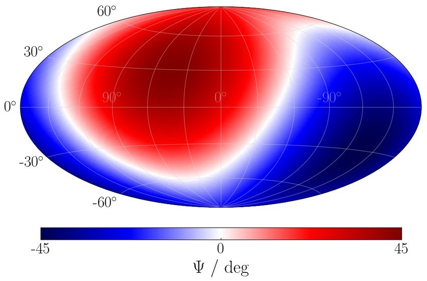
Fit results on realistic scenario
    ✗    Cosmic rays follow AUGER
         energy spectrum, E > 40 EeV

                                                Found cluster
    ✗    Charge uniform up to CNO
         group (Z = 1 … 8)                                      sources
    ✗    4 x 25 signal; 900 isotropic CRs
    ✗    Deflection: JF12 model + blurring

                                             reconstruction
                                                Charge

8       Marcus Wirtz
Evaluate sensitivity on realistic scenario
Signal set 1 set
Statistical measure:
Isotropy set
500 sets
Mean density
in isotropy
9“How to deal with unknown galactic magnetic field?”
Compass methodParametrize new deflection model
JF12 vs PT11
✗ Most important uncertainty in the galactic
magnetic field for cosmic ray deflection
is the directional deflection
✗ Fit parameters for the GMF uncertainties
defined for few fixed points on sphere:
JF12
fit
✗ For the angle of a certain cosmic ray,
interpolate values of the different regions: CR
Using Healpy nside=2 (48 points)
10 as interpolation pointsFit concept
✗ Define ellipses around all observed cosmic rays,
with major axis aligned with the local Psi
by varying the Psi fit parameters
Entropy like cluster loss (minimize “potential energy”)
“Elliptical Fisher distribution”
Penalize too large deviations from model prediction
Fit avoids
values Psi > 90°
11Benchmark simulation
Astrophysical scenario Simulated GMF uncertainty
✗ Auger energy spectrum, E > 40 EeV ✗ Motivated by
✗ differences
4 sources each emitting 25
between
CRs + 900 background CRs
JF12, PT11
✗ Charges uniformly between 1 and 8
✗ Deflection model: ✗ Create a dipolar modulation of the
JF12 galactic field model psi angle, with random direction
+ rigidity dependent smearing and amplitude of 45 degrees
12 Marcus WirtzBenchmark simulation 13 Marcus Wirtz
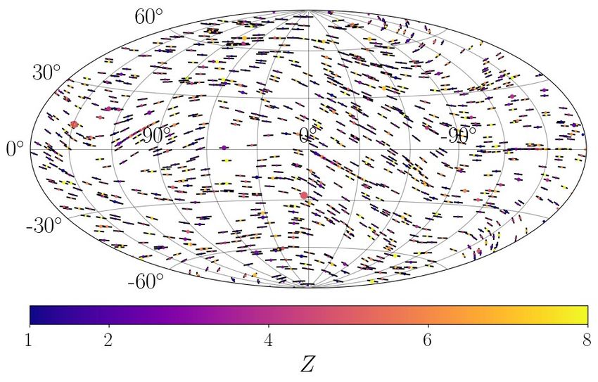
Reconstructed Psi angle for galactic field correction

                                            ✗ Interpolation scheme
                                              provides psi angles
                                              which can change on
                                              intermediate scales
                                            ✗ The psi angles of the
                                              4 sources
                                              [43°, 7°, -4°, -26°]
                                              are well reconstructed

14   Marcus Wirtz
Reconstruction quality
70
60 rmin =2 deg
68-Percentile (∆Ψ / deg)
reference
50 corrected rmin =4 deg
60
rmin =6 deg
40
rmin =8 deg
N
30 50
20
10 40
0
−50 −25 0 25 50 75 10−7 10−6 10−5 10−4
∆Ψ / deg wgmf
✗ Deviation before and after re- ✗ Width of the psi distribution as
construction for 200 scenarios function of the loss weight,
✗ Fit clearly decreases the width for different ellipse widths
of the psi deviation ✗ Scale of roughly 2:1 in the ellipse
15 Marcus Wirtz shape yields best reconstructionSummary
Contracting alignment patterns
✗ Multi-dimensional tensorflow based fit, to contract aligned patterns
in the arrival directions of UHECRs to their sources
✗ Works well on simulated astrophysical scenarios, given that
deflections in the galactic magnetic field are known
Compass method
✗ Approach to fit a deflection model itself by elliptical potentials around
each cosmic ray, which rotate according to the local alignments
✗ First benchmark studies show a promising reconstruction quality
even in high turbulent scattering
16 Marcus Wirtz – mwirtz@physik.rwth-aachen.deBackup
Reliability of galactic                                  JF12

     magnetic field models                   PT11

               R = 10 EV

                                                             R = 10 EV
      Directional differences between GMF models in median
B1    below 40° (remaining offset: blurring)
Fit results on isotropy...
For comparison:
Isotropic backtracking
✗ Cosmic rays follow AUGER
energy spectrum, E > 40 EeV
✗ Charge uniform up to CNO
group (Z = 1 … 8) 10 EV
✗ Arrival directions isotropic
Converged fit result
Run 500 times and
create mean isotropic
5°- tophat map
B2Compass method – Reconstruction on only coherent
300
60 reference
250
reference
corrected 50 corrected
200
40
N
N
150
30
100 20
50 10
0 0
−100 −50 0 50 100 −50 −25 0 25 50 75
∆Ψ / deg ∆Ψ / deg
B3Compass visualization – Toy setup B4
Compass visualization – JF12 model

B5
You can also read


