Investigating the response of leaf area index to droughts in southern African vegetation using observations and model simulations
←
→
Page content transcription
If your browser does not render page correctly, please read the page content below
Hydrol. Earth Syst. Sci., 26, 2045–2071, 2022
https://doi.org/10.5194/hess-26-2045-2022
© Author(s) 2022. This work is distributed under
the Creative Commons Attribution 4.0 License.

Investigating the response of leaf area index to droughts in southern
African vegetation using observations and model simulations
Shakirudeen Lawal1 , Stephen Sitch2 , Danica Lombardozzi3 , Julia E. M. S. Nabel4 , Hao-Wei Wey4 ,
Pierre Friedlingstein5 , Hanqin Tian6 , and Bruce Hewitson1
1 Climate System Analysis Group, Department of Environmental and Geographical Science,
University of Cape Town, Cape Town 7700, South Africa
2 College of Life and Environmental Sciences, University of Exeter, Exeter EX4 4QE, UK
3 National Center for Atmospheric Research, Climate and Global Dynamics,

Terrestrial Sciences Section, Boulder, CO 80305, USA
4 Land in Earth System (LES), Max Planck Institute for Meteorology, Hamburg, Germany
5 College of Engineering, Mathematics and Physical Sciences, University of Exeter, Exeter EX4 4QF, UK
6 School of Forestry and Wildlife Sciences, Auburn University, 602 Duncan Drive, Auburn, AL 36849, USA

Correspondence: Shakirudeen Lawal (lasd_dr@yahoo.com)

Received: 12 October 2020 – Discussion started: 27 November 2020
Revised: 26 March 2022 – Accepted: 28 March 2022 – Published: 27 April 2022

Abstract. In many regions of the world, frequent and con-       summer) season, while the tropical forest biome shows the
tinual dry spells are exacerbating drought conditions, which    weakest response (r = 0.35) at a 6-month timescale in the
have severe impacts on vegetation biomes. Vegetation in         DJF (December–February; hot and rainy) season. In addition,
southern Africa is among the most affected by drought.          we found that the spatial pattern of change of LAI and SPEI
Here, we assessed the spatiotemporal characteristics of me-     are mostly similar during extremely dry and wet years, with
teorological drought in southern Africa using the standard-     the highest anomaly observed in the dry year of 1991, and we
ized precipitation evapotranspiration index (SPEI) over a 30-   found different temporal variability in global and regional re-
year period (1982–2011). The severity and the effects of        sponses across different biomes.
droughts on vegetation productiveness were examined at dif-        We also examined how well an ensemble of state-of-the-
ferent drought timescales (1- to 24-month timescales). In       art dynamic global vegetation models (DGVMs) simulate
this study, we characterized vegetation using the leaf area     the LAI and its response to drought. The spatial and sea-
index (LAI) after evaluating its relationship with the nor-     sonal response of the LAI to drought is mostly overesti-
malized difference vegetation index (NDVI). Correlating the     mated in the DGVM multimodel ensemble compared to the
LAI with the SPEI, we found that the LAI responds strongly      response calculated for the observation-based data. The cor-
(r = 0.6) to drought over the central and southeastern parts    relation coefficient values for the multimodel ensemble are
of the region, with weaker impacts (r < 0.4) over parts of      as high as 0.76 (annual) over South Africa and 0.98 in the
Madagascar, Angola, and the western parts of South Africa.      MAM season over the temperate grassland biome. Further-
Furthermore, the latitudinal distribution of LAI responses      more, the DGVM model ensemble shows positive biases
to drought indicates a similar temporal pattern but different   (3 months or longer) in the simulation of spatial distribution
magnitudes across timescales. The results of the study also     of drought timescales and overestimates the seasonal distri-
showed that the seasonal response across different south-       bution timescales. The results of this study highlight the areas
ern African biomes varies in magnitude and occurs mostly        to target for further development of DGVMs and can be used
at shorter to intermediate timescales. The semi-desert biome    to improve the models’ capability in simulating the drought–
strongly correlates (r = 0.95) to drought as characterized by   vegetation relationship.
the SPEI at a 6-month timescale in the MAM (March–May;

Published by Copernicus Publications on behalf of the European Geosciences Union.
2046                          S. Lawal et al.: Investigating the response of LAI to droughts in southern African vegetation

1   Introduction                                                    calculation (McKee et al., 1993). It is also recognized as ap-
                                                                    propriate for use in southern Africa (Hoffman et al., 2009).
Drought can be described as a natural occurrence whereby            However, the SPI has a significant shortcoming, which is
the natural accessibility of water for a region is beneath the      that its computation uses only rainfall without considering
normal state over a long period of time (Xu et al., 2015).          the effect of other meteorological variables in the develop-
Globally, it is considered one of the world’s most important        ment of drought occurrence (Teuling et al., 2013). In or-
climate risks, with significant environmental, social, and eco-     der to address this shortcoming, the SPEI was developed for
logical impacts on different sectors (e.g. agriculture, forestry,   drought monitoring, and it is regarded as being a more suit-
and hydrology) and human lives (Naumann et al., 2018). In-          able drought index in the region to investigate the spatiotem-
creasing trends in the occurrence and severity of drought in        poral scale of drought (Ujeneza and Abiodun, 2014). SPEI is
West Africa and the Mediterranean have huge impacts on wa-          computed from the difference between potential evapotran-
ter resources and agriculture (Sultan and Gaetani, 2016). In        spiration (PET) and rainfall (Vicente-Serrano et al., 2010).
southern Africa, a region regarded as a climate hotspot be-         PET can be computed using different methods such as the
cause of the projected impacts of climate change on its nu-         Hargreaves (HG) and Penman–Monteith (PM) methods. Al-
merous endemic vegetation, an understanding of these im-            though studies (e.g. Vicente-Serrano et al., 2010) have found
pacts is important for mitigation options in managing future        that the PM method captures drought better than HG, other
drought events. Therefore, it is important to examine drought       studies (e.g. Lawal et al., 2019a) showed that this difference
impacts on vegetation and evaluate how this is simulated in         is negligible over southern Africa.
models.                                                                Many studies have used different indices to quantify ob-
    Drought is a frequent occurrence in southern Africa and         served drought, characterize vegetation, and study drought
has enormous impacts on vegetation in the region. For in-           effects on the productiveness of vegetation across differ-
stance, drought has resulted in a significant loss of biomes        ent timescales. Several studies (e.g. Vicente-Serrano and
and the death of plants (Masih et al., 2014; Hoffman et al.,        National Center for Atmospheric Research Staff, 2015;
2009). It is reported that there has been a significant loss of     Zhang et al., 2012; Lawal et al., 2019a, b) have shown
vegetation cover over the region over the last 30 years (Driver     that the satellite-derived normalized difference vegetation in-
et al., 2012; DEA, 2015). Drought has also impacted the spe-        dex (NDVI) is one the most important indicators of vegeta-
ciation of vegetation thereby causing significant changes to        tion health and greenness. These studies applied NDVI in ex-
the region’s rich biomes through the lack of formation of new       amining drought impacts on global vegetation biomes. How-
species or even the growth of species with underdeveloped           ever, other studies (Gitelson, 2004; Santin-Janin et al., 2009)
morphological and physiological characteristics (Hoffman et         have argued that, while the NDVI is a true proxy for vegeta-
al., 2009). Drought-induced vegetation loss has both ecolog-        tion trends, its potential saturation makes it difficult to fully
ical and socioeconomic consequences for human lives. For            estimate biomass. In addition, because the NDVI parameters
instance, studies have shown that food security in the re-          are not well calibrated and often missing from the models,
gion is threatened due to the continual mortality of vegetation     simulated NDVI can be biased. Due to its high correlation
(FAO, 2000; Müller et al., 2011). Other studies (e.g. Wang,         with NDVI, the leaf area index (LAI) is instead used to char-
2010; Khosravi et al., 2017) have also reported that south-         acterize vegetation conditions (Fan et al., 2008; Zhao et al.,
ern Africa could lose more than USD 200 billion of its GDP          2013). Although the LAI is an important vegetation proxy,
(gross domestic product) from the effects of drought on veg-        it is rarely considered in the estimation of drought impacts
etation. The enormous impacts on vegetation have thus made          on vegetation. Thus, quantifying the response of the LAI to
it imperative to investigate how vegetation might respond to        drought over southern Africa is important for understand-
different drought intensities at varying timescales.                ing the processes that modulate ecosystem services produced
    In order to monitor and quantify drought characteristics,       by vegetation which are crucial for human survival (Melillo,
drought indices are used (Wilhite and Glantz, 1985). Drought        2015).
indices, including the SPI (i.e. the Standardized Precipita-           Previous studies have also evaluated the performance of
tion Index), standardized water-level index, and standardized       coupled climate models in simulating the response of veg-
anomaly index, are derived from a single hydrological vari-         etation to drought. For instance, Lawal et al. (2019a) re-
able, which is rainfall (Kwon et al., 2019). Other indices such     ported that an ensemble of the Community Earth System
as the Palmer drought severity index, multivariate standard-        Model (CESM) showed biases in response simulation of veg-
ized drought index, and standardized precipitation evapotran-       etation to drought. This was attributed to the parameteriza-
spiration index (SPEI) combine two or more variables related        tions of the land component (i.e. community land model –
to other atmospheric or soil and environmental conditions           CLM) which poorly simulated observed NDVI. Given the
that may predispose a plant to water stress (Palmer, 1965;          poor replication of the vegetation response to drought by a
Vicente-Serrano et al., 2010; Hao and AghaKouchak, 2013).           coupled climate model, there is a need to examine land-only
Among the drought indices, the SPI is the most widely used          models and whether they might better capture the drought–
because of the adjustable timescale and its relatively simple       vegetation relationship when the atmospheric forcings are

Hydrol. Earth Syst. Sci., 26, 2045–2071, 2022                                        https://doi.org/10.5194/hess-26-2045-2022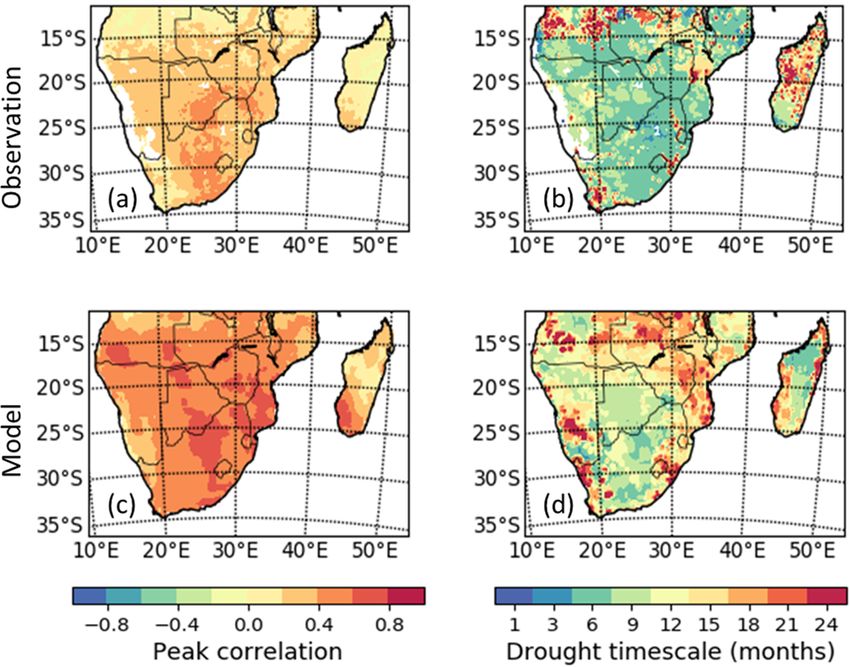
S. Lawal et al.: Investigating the response of LAI to droughts in southern African vegetation                                   2047

derived from observations. The present study used dynamic            ulations. Here we aggregated CRUJRA to monthly samples
global vegetation models (DGVMs) to study the vegetation             and used the data at the same spatial and temporal resolution
response to drought, as little is known about how the LAI            as CRU.
response to drought is simulated by DGVMs. The choice of                For the satellite vegetation indices, first, we used the third
DGVMs is because of their capability to simulate a mostly            generation of NDVI (hereafter, NDVI3g) from the Global In-
accurate carbon exchange between the atmosphere and veg-             ventory Modelling and Mapping Studies (GIMMS), span-
etation ecosystems (Lu et al., 2011).                                ning the period from 1981–2015, with a biweekly tempo-
   The aim of this study is to investigate the response of LAI       ral resolution and a spatial resolution of about 8 km (Pinzon
to droughts in southern African vegetation using observa-            and Tucker, 2014; National Center for Atmospheric Research
tions. We also examined how well the responses are repre-            Climate Data Guide, accessed 2019). Here, we used the data
sented in model simulations. We used satellite-derived and           for the period 1982–2011. Furthermore, we used the third
simulated LAI to quantify vegetation responses to drought.           generation of the GIMMS LAI (LAI3g), which also spans
We characterized the spatiotemporal extent of drought and            the period 1981–2015 and has a biweekly temporal resolu-
its severity using the SPEI and then assessed the influence of       tion and the same spatial resolution as GIMMS3g. The LAI
drought using the LAI from satellite data and model simula-          data had been processed (at source) using a set of neural net-
tions.                                                               works which were first trained on the highest quality and
                                                                     post-processed MODIS LAI and fraction of photosynthet-
                                                                     ically active radiation (FPAR) products and advanced very
2     Data and methodology                                           high resolution radiometer (AVHRR) GIMMS NDVI3g data
                                                                     for the overlapping period (2000 to 2009). The trained neural
2.1    Data                                                          networks were then used to produce the LAI3g and FPAR3g
                                                                     data sets (Mao and Yan, 2019). For the study, LAI3g was also
In this study, we used satellite-calculated (hereafter, ob-          used for the period 1982–2011. We note that GIMMS LAI
served LAI/observation-based LAI) and simulated LAI and              and the NDVI, used in this study, are two different indices.
satellite-derived NDVI, with gridded observation and re-             The LAI was post-processed using different data (MODIS
analysis climate data sets. The gridded observation cli-             LAI, FPAR, and AVHRR NDVI) for the period of 2000–
mate data sets include precipitation and maximum, mean,              2009. The GIMMS LAI product is superior here over the
and minimum temperature. These data were obtained from               GIMMS NDVI, which is due to the information derived from
CRU (i.e. the Climate Research Unit; Mitchell and Jones,             the MODIS LAI. The additional properties on GIMMS LAI
2005; Harris et al., 2014). These are global monthly data            by MODIS differentiate the index from the NDVI. Thus, it
which have 0.5◦ × 0.5◦ as spatial resolution and span the            was necessary to investigate how the two indices differ. In
1901–2019 period. Here, we used the CRU data for the                 addition, other studies (Forkel et al., 2013; Schaefer et al.,
period 1982–2011 to compute observed drought indices                 2012; Rezaei et al., 2016; Lawal et al., 2019a) have inves-
(i.e. SPEI) to characterize the spatiotemporal severity of           tigated how well satellite-derived LAI estimates actual and
drought. CRU is a gridded observed data set, which was used          ground-measured LAI.
because of its suitable spatial and temporal resolutions. Pre-          The simulated monthly LAI data were obtained from 11
vious studies (e.g. New et al., 2000; Otto et al., 2018; Harris      DGVMs which are part of the TRENDY version 7 model
et al., 2020) have shown that there is a good and robust agree-      (Sitch et al., 2008; Le Quéré et al., 2014). These DGVMs
ment between the observation network and CRU over most               are CABLE-POP (Haverd et al., 2018), CLM (Oleson et al.,
parts of southern Africa. We should note that sparseness and         2013), CLASS-CTEM (Melton and Arora, 2016), DLEM
missing data generally affect the correlation between CRU            (Tian et al., 2015), JSBACH (Mauritsen et al., 2018), LPX
and station data in the region. Furthermore, with respect to         (Lienert and Joos, 2018), OCN (Zaehle et al., 2011), OR-
the interannual variability, CRU robustly captures the climate       CHIDEE (Goll et al., 2017), SURFEX (Joetzjer et al., 2015),
factors in southern Africa. The major exception is with the          JULES (Clark et al., 2011), and VISIT (Kato et al., 2013).
long-term trend of precipitation, particularly over the West-        LAI from the models have a monthly temporal resolution
ern Cape province of South Africa and wetter than normal             spanning the period from 1901–2017. We selected these
conditions over the same province. These limitations do not          DGVMs because they have been run with a similar protocol
affect the validity of our results because we are looking at         (S3 simulations) and forcing data sets (i.e. CRUJRA).
below-normal precipitation and temperature.
   The reanalysis climate data we used are the CRUJRA,
which is a combination of CRU and the Japanese Reanaly-
sis data (JRA) (University of East Anglia Climatic Research
Unit; Harris et al., 2020). It is a 6 h land surface, gridded data
with a spatial resolution 0.5◦ × 0.5◦ . CRUJRA was used to
compute reanalysis drought indices and used for model sim-

https://doi.org/10.5194/hess-26-2045-2022                                         Hydrol. Earth Syst. Sci., 26, 2045–2071, 2022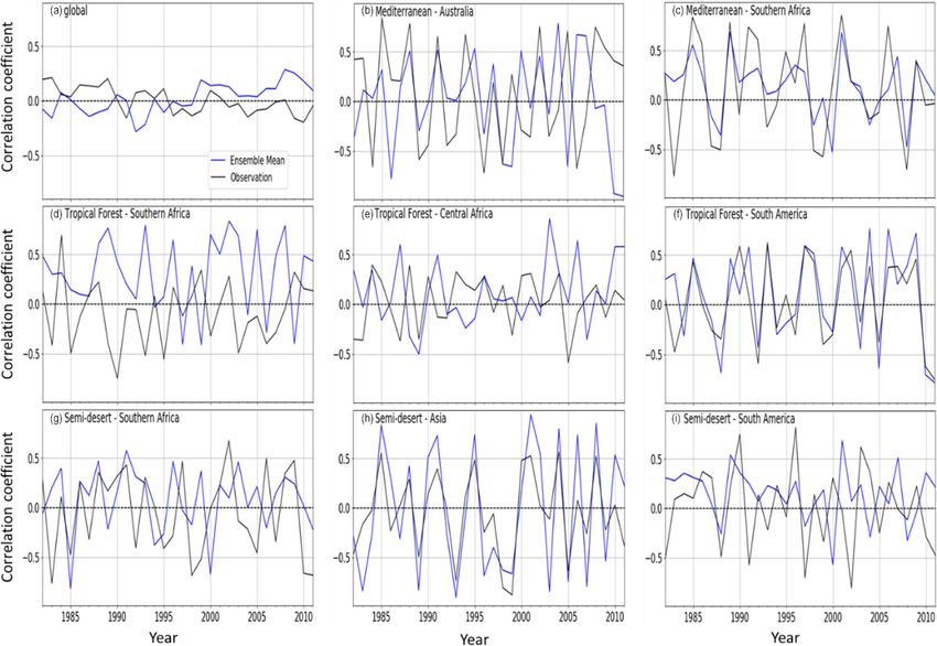
2048                          S. Lawal et al.: Investigating the response of LAI to droughts in southern African vegetation

2.2     Methods overview                                            Table 1. Definition of drought thresholds based on the SPEI scale.

2.2.1    Evaluation of DGVMs and the relationship                                  SPEI                  Drought thresholds
         between NDVI and LAI
                                                                                   2 or more             Extremely wet
The relationship between the NDVI and LAI was evaluated                            1.5 to 1.99           Severely wet
                                                                                   1 to 1.49             Moderately wet
by computing the grid cell spatiotemporal correlation be-
                                                                                   0 to 0.99             Mildly wet
tween GIMMS NDVI and GIMMS LAI. The spatiotemporal                                 0 to −0.99            Mild drought
correlation between GIMMS LAI and simulated LAI from                               −1 to −1.49           Moderate drought
individual DGVMs was also calculated. This was necessary                           −1.5 to −1.99         Severe drought
to show whether LAI is an appropriate estimator of NDVI                            −2 or less            Extreme drought
and how well the models simulate the LAI in the region. Fur-
                                                                                 Sources: Wang et al. (2014) and modified as shown
thermore, we made comparisons of the seasonal values of                          in Lawal (2018).
observed and modelled LAI. We note that the lack of avail-
able of data makes it difficult to compare GIMMS LAI and
actual LAI. Nevertheless, the GIMMS LAI has been evalu-                A time series of the evolution of drought for the 30-
ated and agrees well with observations in other regions (Fan        year period was plotted. The present study extends the time
et al., 2019).                                                      frame for understanding drought impacts from 1982 to 2011,
   The climatology of observed and simulated climatic vari-         mainly because there were frequent droughts in the 2005–
ables, as well as LAI over six major biomes in southern             2011 window (Masih et al., 2014). The time frame was then
Africa for the period 1982–2011, were computed. These               extended back to cover a 30-year period to be long enough
biomes are semi-desert, Mediterranean, dry savanna, moist           to cover the impacts of climate change, which is particu-
savanna, temperate grassland, and tropical forest (Fig. 1; Sin-     larly important considering that southern Africa experiences
clair and Beyers, 2015; Lawal et al., 2019a, b).                    more frequent droughts with impacts exacerbated by cli-
                                                                    mate change. This information is important for considering
2.2.2    Description of drought                                     adaptation measures and understanding the role of climate
                                                                    change.
For the present study, we adopted the definition of meteoro-           The drought index, SPEI, is calculated from the deduc-
logical drought, “which is described as a period (e.g. a sea-       tion between precipitation (P ) and potential evapotranspira-
son) during which there is a deficit in the magnitude of pre-       tion (PET) as follows:
cipitation in a particular area compared to the long-term nor-
mal” (Palmer, 1965; Wilhite and Glantz, 1985). The deficit          D = P − PET,                                                     (1)
in magnitude of precipitation compared to the long-term nor-
mal is mostly accounted for by temperature and less by hu-          where D values represent a measurement of water deficit or
midity, wind, or other variables. Here, we used meteoro-            surplus aggregated at different timescales. D values are ob-
logical drought because it does not make any presumptions           tained through aggregation over individual timescales which
about soil characteristics or runoff. In addition, it is acknowl-   span 1 to 24 months (i.e. 1, 3, 6, 9, 12, 15, 18, 21, and
edged to be a primary component in the depletion of vege-           24 months). The timescales were calculated by including
tation productiveness and the reduction in biomass (Vicente-        the past values of the variable. For example, a timescale of
Serrano et al., 2010). Previous studies (Vicente-Serrano et al.,    15 months suggests that input from the preceding 15 months,
2006; Vicente-Serrano, 2013) have also used meteorological          which includes the present month, was used for calculating
drought in the investigation of drought impacts on biomass          SPEI (Beguería et al., 2014). “For the 1-month timescale,
and vegetation productiveness.                                      only the current month data [are] used for the calculation.
                                                                    The D values were standardized by assuming a suitable
2.2.3    Drought computation and correlation with LAI               statistical distribution (e.g. gamma, log-logistic). The log-
                                                                    logistic distribution was used to standardize the D values in
The analyses include calculating drought (i.e. SPEI) using          this study” (see also Lawal et al., 2019a). For more details
CRU data over a 30-year period (1982–2011) for differ-              on the timescale computation, please see Vicente-Serrano
ent drought timescales. The drought timescale can be de-            et al. (2010; https://rdrr.io/cran/SPEI/man/spei.html, last ac-
scribed as the aggregation of the temporal duration (Vicente-       cess: January 2010). PET is computed from maximum tem-
Serrano et al., 2010). SPEI is an index that is used to quan-       perature, minimum temperature, and mean temperature, us-
tify drought (see Table 1). Therefore, the quantified values of     ing the HG technique (e.g. Vicente-Serrano et al., 2012; Be-
the index give the state of drought in a space. Our definition      guería et al., 2014; Stagge et al., 2014).
and approaches follow numerous previous studies (Vicente-              We note that the PET in the SPEI was computed us-
Serrano, 2013 Vicente-Serrano, 2013; Khosravi et al., 2017;         ing the Hargreaves (HG) method rather than Penman–
Zhao et al., 2013; Hao and AghaKouchak, 2013).                      Monteith (PM) because the data (e.g. vapour pressure and

Hydrol. Earth Syst. Sci., 26, 2045–2071, 2022                                         https://doi.org/10.5194/hess-26-2045-2022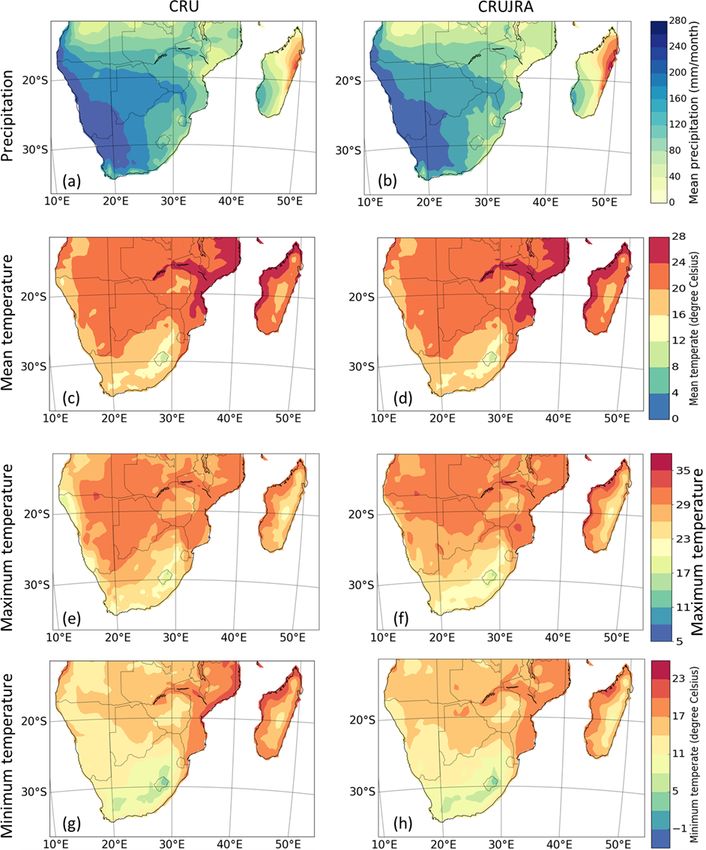
S. Lawal et al.: Investigating the response of LAI to droughts in southern African vegetation                              2049

maximum and minimum humidity) required for comput-                    In summary, CRU was used to compute observed drought
ing PM over southern Africa are sometimes missing or not           while CRUJRA was used to calculate modelled drought be-
available at the needed gridded spatial resolutions and time       cause it is what was used to force the models. This will allow
span. Although PM is considered better in most regions,            for easy observation and model comparisons.
Lawal et al. (2019a) showed that the variation between the            Similar to Lawal et al. (2019a), we calculated the seasonal
PM and HG is negligible for the southern African region.           mean for four seasons, i.e. (a) December, January, and Febru-
The study only considered observed SPEI_PM, which was              ary (DJF), (b) March, April, and May (MAM), (c) June, July,
obtained from https://spei.csic.es/database.html (last access:     and August (JJA), and (d) September, October, and Novem-
January 2010), and not modelled SPEI_PM, due to the un-            ber (SON), from the correlations of monthly series of drought
availability of simulated data required for its computation.       and LAI. These were computed from correlating the monthly
Other studies (e.g. Beguería et al., 2014) have also found that    series (12 series per year) per pixel of GIMMS LAI and each
there is an insignificant contrast in the strength of PM and       monthly series of a 1- to 24-month drought (SPEI) series
HG for reproducing their divergence on measured variables          over the 30-year period with the Pearson correlation. The
such as vegetation indices. We should also note that the SPEI      same technique was used for the model ensemble. In simpler
(unlike SPI or the Palmer drought severity index – PDSI) is        terms, we calculated the correlations (12 sequences in a year)
the most appropriate index for measuring drought in southern       of monthly LAI to the monthly sequences of a 1- to 24-month
Africa, as it accounts for the effect of the evaporative demand    SPEI using 30 years of data. Subsequently, the seasonal mean
from the atmosphere in drought monitoring (Vicente-Serrano         of these correlations was calculated. The peak correlations
et al., 2010; Ujeneza, 2014). In addition, the SPEI is reported    and drought timescales of the models were calculated over
to be able to identify the geographical and temporal coverage      six major biomes in southern Africa, namely (Fig. 1) tem-
of droughts (Vicente-Serrano et al., 2010; Ujeneza, 2014).         perate grassland, tropical forest, moist savanna, dry savanna,
   We deseasonalized GIMMS LAI by transforming the                 semi-desert, and Mediterranean vegetation. These regions
monthly LAI series per pixel to symbolize the standardized         were selected because of their relative importance and are
deviations from the extended mean. This was to make the            most affected by drought.
sequence of LAI commensurate to SPEI (Vicente-Serrano,                Finally, the impacts of extreme events (wet and dry years)
2013) and eliminate the impact of periodicity on vegetation        at different time periods were compared, and the comparison
response. We note that the SPEI is intrinsically deseasonal-       of global and regional responses to drought across biomes for
ized.                                                              the period 1982–2011 was investigated.
   In order to reconcile the difference in the spatial resolu-
tions of CRU and GIMMS, we regridded the data to the same
spatial resolution using the bilinear interpolation method. We     3     Results
then computed the correlation per grid cell between SPEI
(based on CRU) and deseasonalized LAI over the 30-year             3.1    Grid cell correlations between NDVI and LAI
period at the different drought timescales using Pearson cor-
relations. We then compared the spatial distribution of max-       Figure 2 illustrates the relationships between the NDVI and
imum (peak) correlation and the comparable timescales of           LAI for observations, as well as the comparison between ob-
drought for observed SPEI. Our analyses consider the pe-           served and modelled LAI. There is a strong linear relation-
riods at which LAI responds to the presence/absence and            ship between observed NDVI and LAI (Fig. 2a). The cor-
the severity of drought. This is referred to as the drought        relation (0.94) is high between both variables, and the stan-
timescale in the study.                                            dard deviation is low (0.005). The standard deviation being
   Next, we investigated correlations at each grid cell be-        referred to is for GIMMS LAI and individual DGVMs, as
tween the drought (from reanalysis – CRUJRA) and an en-            well as GIMMS LAI and GIMMS NDVI. From the figure, a
semble median of deseasonalized modelled LAI from in-              log-like shape can be seen, where NDVI grows faster when
dividual DGVMs. The peak (maximum) correlations and                LAI is low (< 0.2) and becomes saturated when LAI goes
equivalent timescales from the complete 1- to 24-month             higher (> 0.3). A linear regression of the data shows a slope
timescales were mapped for the ensemble median over the            of 2.15. The low standard deviation indicates that the val-
30-year period. We used the ensemble median because of its         ues from the two indices are close. Although there is a good
lower sensitivity to independent outliers (Reuter et al., 2013).   agreement between observed NDVI and LAI, the 1 : 1 line
In summary, we calculated the model ensemble drought from          shows that the data sets are not exactly equal.
the median from individual members’ drought indices. The              Furthermore, there is good agreement between the ob-
interannual variation in drought impacts on LAI by individ-        served and the simulated LAI (Fig. 2). JULES has the highest
ual DGVMs was also calculated for different timescales. We         correlation (0.97) with observation (Fig. 2l). CLM has the
also examined the observed and ensemble mean of the simu-          weakest (0.73) correlation with the observations (Fig. 2c).
lated LAI response to drought across latitudes.                    DLEM and LPX have the same correlation coefficient value
                                                                   of 0.87 with the observation (Fig. 2e and g). The positive

https://doi.org/10.5194/hess-26-2045-2022                                          Hydrol. Earth Syst. Sci., 26, 2045–2071, 2022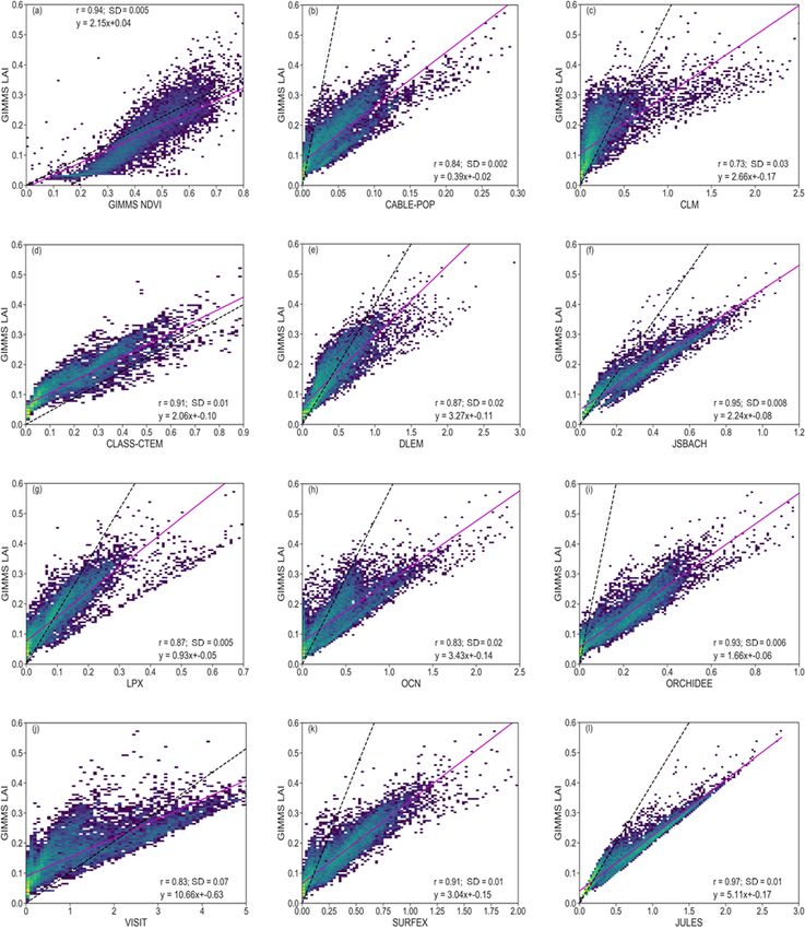
2050 S. Lawal et al.: Investigating the response of LAI to droughts in southern African vegetation
Figure 1. Major vegetation biomes in southern Africa (adapted from UNEP, 2008, Sinclair and Beyers, 2015, and Lawal et al., 2019a, b).
The black lines indicate political boundaries.
relationships between simulated and observed LAI indicate former (Fig. 3u), there is a gradient in the correlation across
a general applicability in investigating the model’s perfor- the region, with higher values in central and southern parts
mance of vegetation response to drought. It also shows that than in Angola and Madagascar. However, with the original
the correlation is strong enough to compare how the LAI re- LAI data (Fig. 3v), the correlation is very high (about 0.85)
acts to drought in the ensemble. An aggregation of the obser- and more prevalent, except in eastern Madagascar and the
vation along the gradient of simulated LAI shows that most Western Cape province of South Africa.
of the models have similar slopes to the observation.
3.3 Climatology of observed and simulated climate
3.2 Seasonal and interannual variations in observed variables and LAI
and modelled LAI
This section compares the seasonal cycle of observa-
The comparison of seasonal and interannual variation of the tional (CRU and CRUJRA) climate variables and observed
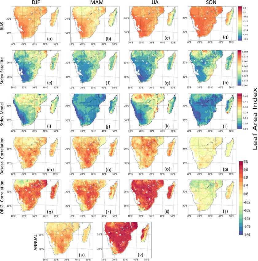
observed and modelled LAI is given in Fig. 3. The model and simulated LAI from GIMMS LAI and TRENDY mod-
shows a stronger positive bias in JJA and SON in comparison els, respectively. Precipitation and temperature are season-
to the summer and winter months and a negative bias over the ally variable, and their climatologies are mostly similar. For
tropical forest region of Madagascar (Fig. 3a–d). In addition, example, precipitation is higher in MAM and DJF over many
the models mostly overestimate the seasonal patterns of LAI of the biomes, except in Mediterranean vegetation, where
in some regions during DJF and JJA and underestimate LAI precipitation is higher in JJA (Fig. 4a, d, g, m, and p). The
in MAM and SON (Fig. 3e–l). Over most parts of the region, wettest month occurs over the TF (i.e. tropical forest biome)
there is a strong correlation and good agreement between the where the precipitation is about 350 mm. Conversely, during
observed and modelled LAI in DJF, MAM, and JJA, although the dry season (JJA), there is little rainfall in the biome, al-
it is weaker in SON (Fig. 3m–t). The strong correlation is though it experiences some precipitation June and July. Over
more prevalent in JJA than other seasons (Fig. 3s), while it the Mediterranean vegetation (Fig. 4j), a winter (JJA) rain-
is weakest in the southern parts of the region. However, the fall region, rainfall variability is lower and is mostly dry in
correlation is largely negative over Angola in DJF and SON DJF and SON. Similarly, the highest minimum and maxi-
(Fig. 3q and t). Furthermore, the correlations between the mum temperature in the region is observed in the DJF season,
model and observed LAI is weaker in deseasonalized data where the highest temperature value exceeds 30 ◦ C. Over the
(hereafter deseas. correlation; Fig. 3m–p) than in original tropical forest biome, although the distribution pattern of pre-
data (hereafter orig. correlation; Fig. 3q–t), thereby showing cipitation and temperature are similar for most months, they
the effects of seasonal patterns on time series data. With re- differ during June and July. The pattern of precipitation and
spect to the period, 1982–2011 (hereafter annual), the corre- temperature distribution generally differs over the Mediter-
lation between the modelled and observed LAI are different ranean vegetation. The pattern of temperature and precipi-
for deseasonalized and original data (Fig. 3u and v). For the tation from CRUJRA follows CRU, although the ensemble
Hydrol. Earth Syst. Sci., 26, 2045–2071, 2022 https://doi.org/10.5194/hess-26-2045-2022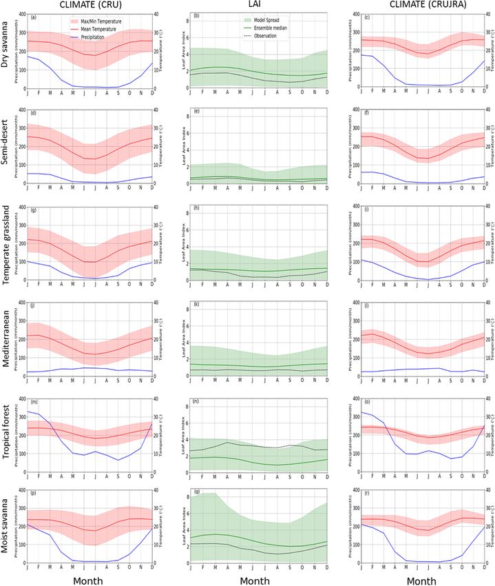
S. Lawal et al.: Investigating the response of LAI to droughts in southern African vegetation                                        2051

Figure 2. Scatterplots of correlations between vegetation indices (observation and model) for the period 1982–2011 over southern Africa.
Inset values indicate the correlation coefficient (r) and standard deviation (SD) between GIMMS LAI and GIMMS NDVI, as well as GIMMS
LAI and modelled LAI. The colour represents each grid cell. The pink solid line is the linear regression, while the dashed black line shows
the 1 : 1 line. The unequal x axes are to visualize the detailed data for the models.

https://doi.org/10.5194/hess-26-2045-2022                                             Hydrol. Earth Syst. Sci., 26, 2045–2071, 2022
2052                          S. Lawal et al.: Investigating the response of LAI to droughts in southern African vegetation

Figure 3. Spatial seasonal distribution and interannual variability (IAV) of satellite-calculated and modelled LAI (multimodel mean) over
southern Africa. Panels (a–d) show the difference (bias). Panels (e–h) and (i–l) show their standard deviation (SD). Panels (m–p) show the
correlations between deseasonalized GIMMS LAI and modelled LAI. Panels (q–t) show their correlations for original GIMMS LAI and
modelled LAI. Panels (u) and (v) show correlations between GIMMS LAI and modelled LAI but for the period 1982–2011. The interannual
variability for observed and modelled LAI for the period 1982–2011 is shown in Fig. S8.

spread is much narrower (Fig. 4c, f, i, l, o, and r). The spa-         although it shows some biases in magnitudes and for mini-
tial patterns of the climate variables from CRU and CRUJRA             mum temperature (Fig. 5g and h).
are shown in Fig. 5. CRUJRA simulates the pattern of pre-                 There is not a strong seasonality for LAI, with maximum
cipitation over southern Africa well (Fig. 5a and b) as CRU,           observed LAI values being less than 4 in all biomes. The
                                                                       models reproduce the climatology of LAI over the southern

Hydrol. Earth Syst. Sci., 26, 2045–2071, 2022                                            https://doi.org/10.5194/hess-26-2045-2022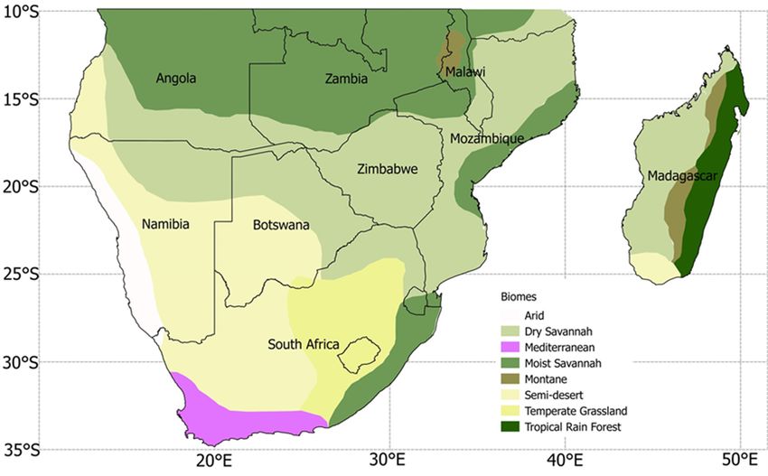
S. Lawal et al.: Investigating the response of LAI to droughts in southern African vegetation                                  2053

Figure 4. Annual cycle of observed climate variables (precipitation in millimetres per month; maximum, minimum, and mean temperature
in degrees Celsius) and LAI for observation and multimodel mean (TRENDY) across six southern African biomes for the period 1982–2011.
The annual cycle of the LAI for individual models is shown in Fig. S5.

https://doi.org/10.5194/hess-26-2045-2022                                         Hydrol. Earth Syst. Sci., 26, 2045–2071, 2022
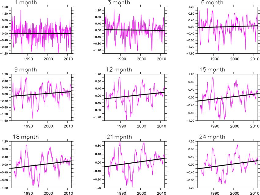
2054                          S. Lawal et al.: Investigating the response of LAI to droughts in southern African vegetation

Figure 5. Spatial distribution of precipitation, mean temperature, maximum temperature, and minimum temperature over southern Africa in
CRU and CRUJRA for the period 1982–2011.

African biomes well, with a few exceptions (Fig. 4b, e, h, k, n       3.4   The evolution of drought in southern Africa
and q). For instance, the models simulate the drop in LAI
over the semi-desert, temperate grassland, tropical forest, dry       Figure 6 shows the evolution of observed SPEI in southern
savanna, and moist savanna biomes in JJA. The highest in-             Africa between 1982 and 2011. Here, drought indices from
crease in observed LAI occurs over the tropical forest in             CRUJRA are not included because a preliminary investiga-
April, although the models simulate a decrease in LAI over            tion showed close magnitudes for drought indices computed
tropical forest during this time. On the other hand, the lowest       from CRU and CRUJRA. We note that CRU was used to cal-
amount (less than 0.1) of LAI is observed in September, and           culate SPEI for the observation, while simulated SPEI was
this occurs over the semi-desert biome. Observations typi-            computed with CRUJRA.
cally fall within the range of the model ensemble. In addition,          There is interannual, seasonal, and decadal variability in
the distribution pattern of the simulated LAI is similar to the       the drought indices during dry and wet conditions over south-
observation in most biomes except in the Mediterranean and            ern Africa. Although 1-, 3-, and 6-month SPEI indicate no
tropical forest biomes. The LAI pattern also follows that of          trend in wet or dry spells, they show the intensity of drought
the climatic variables, although the former lag. The lag effect       events for the 30-year period (Fig. 6a–c). The highest mag-
is accounted for in this study and is known as the drought            nitude of the drought is captured by a 1-month SPEI while
timescale.                                                            the lowest is shown in a 21-month SPEI. The severity of the

Hydrol. Earth Syst. Sci., 26, 2045–2071, 2022                                          https://doi.org/10.5194/hess-26-2045-2022
S. Lawal et al.: Investigating the response of LAI to droughts in southern African vegetation                                      2055

Figure 6. Evolution of SPEI in southern Africa for the period 1982–2011. The trend is significant at the 90 % confidence interval for all
timescales.

drought intensity is similar for all SPEI (i.e. 1- to 24-month         be much stronger, i.e. in the 0.6–0.8 range for most of the
SPEI). The magnitude of the severity is on the y axis of the           regions. In addition, over the arid areas of Namibia, mod-
1- to 24-month SPEI.                                                   els simulate a LAI, while observations depict no measurable
   We note an increasing trend in SPEI (9 to 24 months). Ta-           LAI, indicating that models simulate the LAI in areas where
bles 2 and 3 illustrate when droughts occurred and the sever-          observations show no measurable LAI.
ity of the droughts within the 30-year period. They also show,            The multimodel median has a drought timescale that is
however, that droughts were most frequent and intense in the           mostly longer than the observations (Fig. 7b and d). For in-
second decade, thus, indicating how climate change is ex-              stance, the drought response of simulated LAI occurs mostly
pected to increase the frequency and severity of droughts.             over a longer time period (6- and 9-month timescale) than
                                                                       in the observation over eastern Madagascar. Over the south-
3.5   Spatial distribution of LAI response to drought and              ern areas of Madagascar and central Zambia, the multimodel
      the timescales                                                   median overestimates the drought timescale. Over the cen-
                                                                       tral areas of South Africa and Mozambique, simulated LAI
                                                                       responds at intermediate (9-month) timescales. In compari-
Figure 7 presents the spatial distribution of the peak corre-
                                                                       son, similar drought timescales for the observation and the
lation between the SPEI and the LAI and the timescales at
                                                                       model ensemble median are shown in parts of Angola.
which the correlation occurs. This is to show the magnitude
of response of LAI to drought in southern Africa and the
length of the period for the response.                                 3.6   Latitudinal distributions of LAI response to
   Observations show that southern African LAI can respond                   drought and the timescales
fairly strongly to droughts (peak correlation magnitudes of
between 0.4 and 0.6), though the response is much weaker
(r < 0.4) in eastern Madagascar, Angola, and parts of South            The present study investigated and discussed the implications
Africa (Fig. 7a). The TRENDY multimodel median generally               of drought on different vegetation/biome types across lati-
overestimates the observed magnitude of the LAI to drought             tudes in the region. Here, we stratified the LAI response to
response (Fig. 7c). Peak correlations for the models seem to           drought based on latitude because we intend to investigate

https://doi.org/10.5194/hess-26-2045-2022                                            Hydrol. Earth Syst. Sci., 26, 2045–2071, 2022
2056 S. Lawal et al.: Investigating the response of LAI to droughts in southern African vegetation
Table 2. Characteristics of drought occurrence for a 1- to 24-month drought timescale for the first decade (1982–1991), second decade (1992–
2001), and third decade (2002–2011).
Drought Number of drought events Year of moderate drought events
timescale First Second Third First Second Third
decade decade decade decade decade decade
1 month 53 62 53 1987 1992, 1990 2004, 2007, 2008, 2011
3 months 55 64 58 1988 1991, 1992 2004, 2008, 2011
6 months 44 62 60 1982 1992, 1993 2004
9 months 55 66 62 – 1992, 1994 –
12 months 53 68 56 – 1992, 1995 –
15 months 58 63 56 – 1992 –
18 months 54 69 51 – 1992, 1994 –
21 months 51 69 56 – 1992, 1995 –
24 months 41 71 54 – 1992, 1994 –
Table 3. Statistics of the severity of drought for 1- to 24-month drought timescale for first decade (1982–1991), second decade (1992–2001),
and third decade (2002–2011). SD is the standard deviation, and max is the highest magnitude of drought occurrence.
Drought Mean SD Max
timescale First Second Third First Second Third First Second Third
decade decade decade decade decade decade decade decade decade
1 month 0.30 0.39 0.31 0.26 0.26 0.27 1.1 1.02 1.15
3 months 0.32 0.36 0.29 0.24 0.25 0.25 1.02 1.01 1.12
6 months 0.38 0.38 0.26 0.31 0.28 0.24 1.04 1.3 1.33
9 months 0.31 0.41 0.21 0.26 0.35 0.18 0.86 1.32 0.83
12 months 0.30 0.43 0.21 0.21 0.35 0.18 0.81 1.27 0.7
15 months 0.28 0.47 0.20 0.21 0.31 0.18 0.77 1.13 0.7
18 months 0.27 0.48 0.20 0.17 0.28 0.12 1.02 1.02 0.77
21 months 0.18 0.50 0.17 0.2 0.28 0.14 0.62 1.00 0.61
24 months 0.28 0.51 0.15 0.19 0.24 0.11 0.55 0.93 0.46
and identify the shift in the response based on the vegetation 3.7 Response of LAI to droughts across seasons
types across the latitudinal belt.
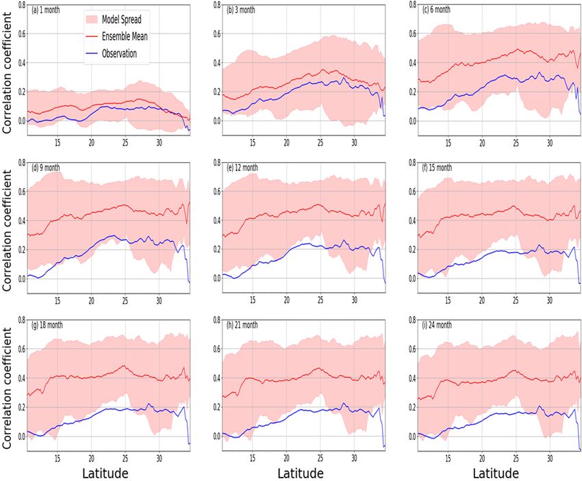
While the pattern of the latitudinal distribution of the LAI Observations show similar correlations between LAI and
response to drought is identical across different timescales, drought across all seasons in the biomes (Fig. 9). For the dry
the magnitudes generally differ (Fig. 8). The response is savanna, which is one of the most climate-impacted biomes
much weaker (less than 0.15) for the 1-month timescale in the region, LAI response to drought is strong, the correla-
than for other timescales. The strongest response is observed tion is as high as 0.8 in MAM season, and it occurs at a 12-
at a 6-month timescale between latitudes of 25 and 30◦ . month timescale. The correlations between drought and LAI
The model ensemble mean generally agrees with the pat- are also very strong in other seasons over the same biome
tern of the observed LAI–SPEI correlations across all the and occur at 6- and 12-month drought timescale, except over
timescales. However, the magnitudes differ from the ob- the Mediterranean vegetation, where the response occurs at
servation. The modelled correlation is stronger than ob- 18 months in the DJF season. Similarly, the peak correlations
servations for the longer (6 months or more) timescales. between drought and LAI are strong across the other biomes.
This means that the models are oversimplifying how the With the exception of the tropical forest biome, the drought
LAI responds to drought by neglecting other climate fac- timescale is at longer time periods (> 6 months).
tors, such that, in models, LAI only correlates to the water The model ensemble generally overestimates correlations
deficit (SPEI). Furthermore, there is an offset between the across the biomes in different seasons. While the correlation
observation and model mean, which is consistent across most magnitude remains mostly larger than the observation, mod-
of the timescales, perhaps due to the strong memory of the els nonetheless simulate a closer correlation with observa-
some of the models. tion in some biomes and seasons. For instance, over Mediter-
ranean vegetation, models simulate a fairly good response
Hydrol. Earth Syst. Sci., 26, 2045–2071, 2022 https://doi.org/10.5194/hess-26-2045-2022S. Lawal et al.: Investigating the response of LAI to droughts in southern African vegetation 2057
the highest correlation value. Furthermore, JSBACH simu-
lates the highest correlation value for most of the timescales,
while CLM simulates the lowest correlation values for most
(3, 9, 12, 15, and 18 months) of the timescales. A possible
reason for the weak performance of CLM may be its repre-
sentation of the canopy construction of the plant functional
types (PFTs) and of its foliage clumping representation. In
addition, CLM is limited in its simulations of vegetation with
regards to transpiration, due to the rooting depth, among oth-
ers (Dahlin et al., 2020). Furthermore, CLM does not simu-
late savanna ecosystems well but instead uses a combination
of grasses, shrubs, and trees. There are also some problems
(such as an unusual green-up in the dry season) identified
with deciduous stress responses (Dahlin et al., 2015).
3.9 Impacts of extreme events on LAI
Figure 7. Spatial distribution of peak correlation between
drought (SPEI) and LAI over the region of southern Africa in the The impacts of extreme events on LAI are shown in Fig. 10.
observation and in the model ensemble median for the period 1982– The objective was to discuss the impacts and compound in-
2011. Panels (a) and (c) show the peak correlation per pixel, which fluences of extreme events on LAI during extremely hot/dry
is independent of the timescale and the month of the year. Panels and wet years. Here, extreme events are the wet (2000, 2010,
(b) and (d) indicate the timescales at which the peak correlation be- and 2011) years, i.e. the periods with precipitation higher
tween SPEI and LAI is found. Areas with no significant correlation than normal, and the dry (1983, 1984, and 1991) years, which
are white. include the periods of very high dry spells. To achieve this,
we used the anomaly of precipitation, SPEI, and LAI rela-
tive to the long-term mean. The anomaly was computed as
of LAI to drought in all seasons. Furthermore, in nearly a difference between a particular extremely dry or wet year
all other biomes, the ensemble spread overlaps with the ob- and 30-year mean representing dry and wet conditions. The
servations. In addition, simulations mostly overestimate the anomaly is the magnitude of impacts added by the extreme
drought timescale, except over dry savanna. A possible rea- event in a particular year. The spatial pattern of the changes in
son for why the difference in the timescale for dry savanna LAI, SPEI, and precipitation were then plotted. Our analyses
was underestimated may be because phenological triggers follow Pan et al. (2015). Furthermore, we computed the pat-
for dry savannah vegetation types respond differently to en- tern correlation coefficients (r) between the LAI and climate
vironmental variables, which the models do not capture. The variables for each extremely dry and wet year. The statistical
African dry savanna region is characterized by rapid vegeta- significance of the coefficients was also calculated. The goal
tion changes due to fire, land use, among others, and senes- of this is to ascertain whether the sign of the anomaly of the
cence for prolonged dry periods (Rahimzadeh-Bajgiran et variables correspond in the same locations on two different
al., 2012; Zhu and Liu, 2015), which may have contributed maps. In order to determine the significance of correlation
to the underestimation in the response of the models. Sim- coefficient, we performed the linear regression t test (i.e. Lin-
ilarly, models have different representations of fire, which RegTTest). This finds the best line of fit among a set of data
could also indirectly contribute to the underestimated model points. It also checks the quality of the fit by carrying out a
responses to drought. t test on the slope, thus testing the null hypothesis that the
best fitted line is 0, suggesting that there is no correlation be-
3.8 Interannual variation in the model simulation of tween two variables, since an association with a slope of zero
the drought impacts on LAI implies that one variable does not affect the other. Therefore,
if the p value is not sufficiently low, then we do not have suf-
Table 4 shows the correlations between observed mean SPEI ficient data to accept relationship between the variables. For
and LAI for the period 1982 and 2011 and simulations by this study, we used a significance level of 5 % i.e. α = 0.05,
individual DGVMs across different timescales. Unlike Fig. 7, which is the most commonly used value in life and biolog-
which shows the peak correlations, the table shows the mean ical sciences. We then tested the hypothesis on whether the
correlation for the 30-year period. p value is less than the significance level (α = 0.05), which
There is variation in the interannual simulation of LAI is our null hypothesis. In cases where that is the case, we
response to drought across different timescales by individ- rejected the null hypothesis and concluded that there is ad-
ual models. For instance, on the 1-month timescale, JULES equate evidence that there is a significant linear relationship
simulates the lowest correlation value while JSBACH shows between the variables i.e. LAI–SPEI and LAI–precipitation.
https://doi.org/10.5194/hess-26-2045-2022 Hydrol. Earth Syst. Sci., 26, 2045–2071, 20222058 S. Lawal et al.: Investigating the response of LAI to droughts in southern African vegetation
Figure 8. Mean correlation (observed and multimodel ensemble) of annual LAI and SPEI for 1982–2011 across latitudes over southern
Africa for 1- to 24-month timescales.
Table 4. Model simulation of mean SPEI and LAI correlations between 1982 and 2011. The asterisk (∗ ) indicates the model with the lowest
mean correlation.
Correl. GIMMS CABLE- CLM CLASS- DLEM JSBACH LPX OCN ORCHIDEE SURFEX JULES VISIT
LAI POP CTEM
1 month 0.0066 0.1017 0.1188 0.1266 0.085 0.1388 0.0842 0.0579 0.0884 0.1094 0.027∗ 0.086
3 months 0.0775 0.3084 0.0187∗ 0.29 0.2499 0.4165 0.2403 0.1644 0.266 0.2791 0.1434 0.1108
6 months 0.091 0.3474 0.1806 0.3562 0.3305 0.5404 0.2386 0.3377 0.3733 0.3759 0.2429 0.1703∗
9 months 0.0832 0.333 0.2034∗ 0.3496 0.3437 0.5734 0.2505 0.4055 0.39 0.3994 0.3189 0.23
12 months 0.0813 0.3053 0.2155∗ 0.3231 0.3229 0.5398 0.304 0.4109 0.4054 0.3911 0.3663 0.2892
15 months 0.0642 0.2773 0.2161∗ 0.2912 0.2846 0.4925 0.3208 0.4106 0.4132 0.3547 0.3623 0.3198
18 months 0.0452 0.2534 0.2349∗ 0.276 0.2381 0.4599 0.2405 0.3998 0.4109 0.3289 0.3586 0.3472
21 months 0.0406 0.239 0.2402 0.27 0.2119 0.4334 0.1569∗ 0.3739 0.3962 0.2955 0.3621 0.3501
24 months 0.0409 0.2302 0.2355 0.2668 0.2186 0.4696 0.2064∗ 0.3528 0.3777 0.2682 0.3617 0.327
In cases where the p value is greater, we do not reject the null evaporate from the soil. SPEI, as a drought index, considers
hypothesis, since there is not enough evidence to conclude on temperature effects on moisture availability.
the significance of correlation coefficients. We considered only observation, i.e. CRU (precipitation
Note that, although the SPEI is a drought index, it was also and drought) and satellite-calculated LAI. The observed cli-
considered in a wet year because the impact of drought usu- mate (CRU) data are not sub-monthly. Only the CRUJRA
ally lasts beyond a dry year, especially in semi-arid regions (reanalysis), which was used for model correlation, is sub-
of southern Africa. In addition, the hot temperature has an in- monthly. The model was not analysed in this section because
fluence on the worsening of the drought by causing water to our goal was simply to examine the observed impacts (or in-
fluence) of an extreme event.
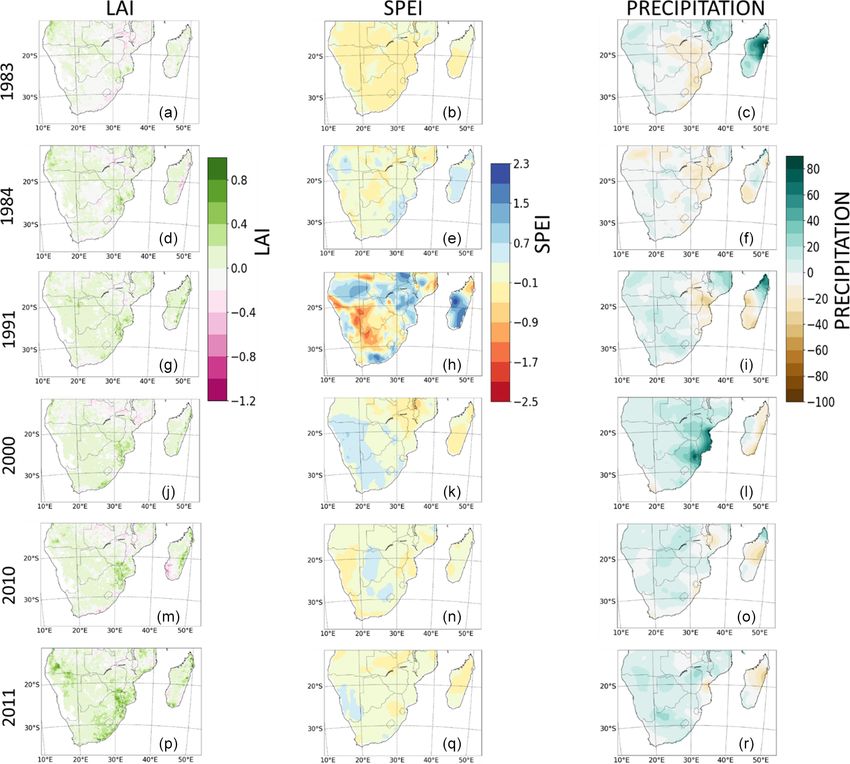
Hydrol. Earth Syst. Sci., 26, 2045–2071, 2022 https://doi.org/10.5194/hess-26-2045-2022S. Lawal et al.: Investigating the response of LAI to droughts in southern African vegetation 2059 Figure 9. Seasonal correlations of drought (SPEI) and LAI across six southern African biomes. The values on the left axis show the peak correlation in observation and TRENDY models. The values on the right axis indicate the corresponding drought timescale. The spatial pattern of change of LAI and SPEI are mostly change of the SPEI in the region is observed in the dry year similar during extreme dry and wet years (Fig. 10). For ex- of 1991 (Fig. 10h). However, the pattern of change of the ample, in 1983 (a dry year), the negative anomaly of LAI LAI and SPEI are not similar over some regions in some pe- in some parts of the region largely follows the negative riods. For instance, in 1991, while a negative anomaly of the anomaly of the SPEI, except in the western and central parts SPEI is observed in northern Madagascar and central parts (Fig. 10a and b). In 1984, both variables show a strong posi- of southern Africa, LAI shows a positive anomaly (Fig. 10g tive anomaly over Madagascar, Eswatini, and the KwaZulu- and h). The opposite and decreasing relationship between the Natal province of South Africa (Fig. 10d and e). The pat- two variables in 1991 is also evident in the pattern correla- tern of change of both SPEI and LAI are also comparable tion coefficient value of −0.16 (Fig. 10h). The variation in during the extremely wet year. In the wet year of 2000, the anomaly in these parts and period may be due to the exertion positive anomaly of SPEI that is observed in Namibia and of a stronger influence by other factors such as residual soil South Africa is also evident for the LAI (Fig. 10j and k). In moisture and precipitation (see Fig. 10i), with temperature a like manner, both variables show a negative anomaly over having negligible impacts. Malawi and Zambia. The strongest pattern (magnitudes) of https://doi.org/10.5194/hess-26-2045-2022 Hydrol. Earth Syst. Sci., 26, 2045–2071, 2022
2060                            S. Lawal et al.: Investigating the response of LAI to droughts in southern African vegetation

Figure 10. Spatial pattern changes in satellite-calculated LAI, observed SPEI, and precipitation during extremely dry (1983, 1984, and 1991)
and wet (2000, 2010, and 2011) years. For panels (a–i), the changes in LAI, SPEI, and precipitation were calculated as a difference between
the dry year and the 30-year mean. For panels (j–r), changes in LAI, SPEI, and precipitation were calculated as the difference between the
wet year and the 30-year mean. White areas indicate no correlation. The pattern correlation coefficients and the statistical significance of the
coefficients between the variables are given in Table 5.

   The influence of precipitation (as a standalone meteoro-               parts of southern Africa, there is a decrease in the LAI, as is
logical factor) on LAI during extreme events is limited. This             the case with SPEI (Fig. 10j–l). Nevertheless, precipitation
is observed from the disparity in the spatial pattern of the LAI          plays a primary/major role in the pattern of change of LAI,
and precipitation over some regions and periods. For exam-                as is observed over the most parts of the region during the
ple, in 1984, the wide negative anomaly of precipitation that             years considered.
is shown over Zimbabwe, Mozambique, and southern Mada-                       Generally, the pattern correlation coefficient values be-
gascar is opposite to the LAI, which shows positive anomaly               tween the LAI and SPEI are higher than those between
(Fig. 10d and f). The LAI anomaly is more similar to that of              the LAI and precipitation in extremely dry and wet years
the SPEI (Fig. 10e). Also, in wet year of 2000, while precip-             (Table 5). Although the coefficients are small, they are
itation shows a preponderant increase over the northeastern               mostly significant across the different extreme periods, ex-

Hydrol. Earth Syst. Sci., 26, 2045–2071, 2022                                                https://doi.org/10.5194/hess-26-2045-2022
S. Lawal et al.: Investigating the response of LAI to droughts in southern African vegetation                                2061

cept for 1983, an extremely dry year, where the p value            both vegetation indices differ temporally and seasonally over
is 0.58 for LAI–SPEI (Table 5). The extremely low statistical      deciduous forests, which are sometimes not accounted for in
significance indicate low standard errors and a large number       models that test their relationship (Wang et al., 2004). For in-
of grid sizes for the region.                                      stance, while the relationship is strong during periods of leaf
                                                                   production and senescence, no relationship is observed dur-
3.10    Comparison of global and regional distribution of          ing the period of leaf constant due to NDVI saturation above
        LAI response to droughts (1982–2011)                       certain LAI values (Xue and Su, 2017).
                                                                      Although the present study found a strong linear relation-
There is variability in the global and regional temporal dis-      ship between the NDVI and LAI in southern Africa, other
tribution of the LAI response to drought (at a 12-month            studies (Potithep et al., 2010; Towers et al., 2019) have shown
timescale) when global vegetation biomes are split into re-        that the two indices are not always directly proportional. For
gional biomes (Fig. 11). The map of the global biomes is           example, both indices do not exhibit the same relationships
shown in Fig. S1 in the Supplement. The observed global            over different ecoregions such as the evergreen broadleaf for-
response indicates a decreasing trend of the LAI response to       est or deciduous needleleaf forest. Furthermore, other studies
drought, while the model mean shows an increasing estimate.        (Fan et al., 2008; Tian et al., 2017) found that the LAI may
   The semi-desert biome dominates the LAI response                be a better indicator of plant biomass and health because of
as higher drought–vegetation correlations are observed             the saturation associated with the NDVI, particularly in the
(Fig. 11g–i). Over the biome, there is a more marked interan-      drylands. This makes the LAI more applicable in monitoring
nual variability, which makes the biome an important player        the vegetation response to drought. Evaluating how the LAI
in the global carbon cycling (Poulter et al., 2014). The re-       differs from the NDVI over different biomes (such as dry sa-
sponse over the semi-desert in southern Africa is, however,        vanna, tropical forest, etc.), with regards to temporal differ-
weaker in comparison to the other semi-desert biomes.              ence, is shown in Fig. S7. Both the LAI and NDVI show simi-
   The response over the Mediterranean vegetation in Aus-          lar annual cycles over southern Africa, except for the tropical
tralia is stronger than the Mediterranean vegetation over the      forest and Mediterranean vegetation.
rest of inland southern Africa. Over the biome, the model
simulates closer magnitudes in the latter than over Australia      4.2   The importance of sub-monthly data in drought
(Figs. 11b and 9c).                                                      computation and monitoring
   Over the tropical forest biomes, there is a weaker response
in central Africa compared to southern Africa and South            The data used to evaluate drought indices are CRUJRA. JRA
America; the model simulates the closest response in mag-          is a reanalysis data set and has a 6 h temporal resolution. Ad-
nitude in South America (Fig. 11d and f).                          ditionally, CRUJRA have the data used to force the DGVMs,
                                                                   so the drought indices are being calculated based on the same
                                                                   data the models use for their simulations. JRA is a reanal-
4     Discussion                                                   ysis data set, but the combined CRUJRA product uses the
                                                                   sub-monthly information from JRA and is constrained to the
4.1    Relationship of LAI to phenological changes
                                                                   monthly CRU observations. The comparisons of the data are
LAI is a variable that is needed for the global modelling of       shown in Figs. 5 and S6. It is useful to use data with shorter
biogeochemistry, climate, ecology and hydrology, and differ-       times because the study focuses on an evaluation of drought
ent primary production models (e.g. Running and Coughlan,          impact, which is sensitive to the timescale. In the drylands,
1988; Sellers et al., 1996; Bonan et al., 2002). In view of the    for instance, the uncertainties associated with monthly data
need to run biogeochemical models at regional and global           in drought monitoring are reduced when sub-monthly data
scales, accurate LAI data at moderate to high resolutions are      are used (Mukherjee et al., 20117). With regards to the pre-
crucial (Wang et al., 2004). The relationship between NDVI         cipitation and temperature fields, the difference is negligible.
and LAI is applied as a support algorithm in MODIS LAI.               We note that, over different parts of the world, CRU
Thus, from the viewpoint of the availability of data, retriev-     has been widely validated against station data (Harris et
ing LAI from analysing the NDVI–LAI relationship remains           al., 2020), and there is a high accuracy of the valida-
the main perspective for high temporal resolution in regional      tion. Therefore, observed SPEI gives a high accuracy of
and global studies (Wang et al., 2004).                            measured drought. Another major advantage of using the
   LAI showed a linear relationship with NDVI. This sug-           observational-based CRU data is its spatial and temporal cov-
gests that the NDVI is associated with the phenological            erage. Station data are available for very few points and for
changes in plants, the parts of the surface cover class which      limited times in the region of interest. The few data that are
contribute to the general reflectance, and the variations in the   available are fraught with missing data, rendering them an
angle of solar zenith (Wang et al., 2004). Studies (e.g. My-       unreliable data source (Harris et al., 2020).
oung et al., 2013) have, however, found that the relationship
between NDVI and LAI varies intra- and interannually, and

https://doi.org/10.5194/hess-26-2045-2022                                       Hydrol. Earth Syst. Sci., 26, 2045–2071, 2022
You can also read


