Lévy noise versus Gaussian-noise-induced transitions in the Ghil-Sellers energy balance model
←
→
Page content transcription
If your browser does not render page correctly, please read the page content below
Nonlin. Processes Geophys., 29, 183–205, 2022
https://doi.org/10.5194/npg-29-183-2022
© Author(s) 2022. This work is distributed under
the Creative Commons Attribution 4.0 License.

Lévy noise versus Gaussian-noise-induced transitions in the
Ghil–Sellers energy balance model
Valerio Lucarini1,2,z , Larissa Serdukova1,2 , and Georgios Margazoglou1,2
1 Department   of Mathematics and Statistics, University of Reading, Reading, UK
2 Centre for the Mathematics of Planet Earth, University of Reading, Reading, UK
z Invited contribution by Valerio Lucarini, recipient of the EGU Lewis Fry Richardson Medal 2020.

Correspondence: Valerio Lucarini (v.lucarini@reading.ac.uk)

Received: 20 October 2021 – Discussion started: 5 November 2021
Revised: 17 March 2022 – Accepted: 5 April 2022 – Published: 11 May 2022

Abstract. We study the impact of applying stochastic forcing      attractor. This property can be better elucidated by consider-
to the Ghil–Sellers energy balance climate model in the form      ing singular perturbations to the solar irradiance.
of a fluctuating solar irradiance. Through numerical simula-
tions, we explore the noise-induced transitions between the
competing warm and snowball climate states. We consider
multiplicative stochastic forcing driven by Gaussian and α-       1     Introduction
stable Lévy – α ∈ (0, 2) – noise laws, examine the statistics
of transition times, and estimate the most probable transition    1.1    Multistability of the Earth’s climate
paths. While the Gaussian noise case – used here as a refer-
                                                                  The climate system comprises the following five interacting
ence – has been carefully studied in a plethora of investiga-
                                                                  subdomains: the atmosphere, the hydrosphere (water in liq-
tions on metastable systems, much less is known about the
                                                                  uid form), the upper layer of the lithosphere, the cryosphere
Lévy case, both in terms of mathematical theory and heuris-
                                                                  (water in solid form), and the biosphere (ecosystems and
tics, especially in the case of high- and infinite-dimensional
                                                                  living organisms). The climate is driven by the inhomoge-
systems. In the weak noise limit, the expected residence time
                                                                  neous absorption of incoming solar radiation, which sets up
in each metastable state scales in a fundamentally different
                                                                  nonequilibrium conditions. The system reaches an approxi-
way in the Gaussian vs. Lévy noise case with respect to
                                                                  mate steady state, where macroscopic fluxes of energy, mo-
the intensity of the noise. In the former case, the classical
                                                                  mentum, and mass are present throughout its domain, and
Kramers-like exponential law is recovered. In the latter case,
                                                                  entropy is continuously generated and expelled into the outer
power laws are found, with the exponent equal to −α, in ap-
                                                                  space. The climate features variability on a vast range of spa-
parent agreement with rigorous results obtained for additive
                                                                  tial and temporal scales as a result of the interplay of forcing,
noise in a related – yet different – reaction–diffusion equa-
                                                                  dissipation, feedbacks, mixing, transport, chemical reactions,
tion and in simpler models. This can be better understood
                                                                  phase changes, and exchange processes between the subdo-
by treating the Lévy noise as a compound Poisson process.
                                                                  mains (see Peixoto and Oort, 1992, Lucarini et al., 2014a,
The transition paths are studied in a projection of the state
                                                                  Ghil, 2015, and Ghil and Lucarini, 2020).
space, and remarkable differences are observed between the
                                                                     In the late 1960s Budyko (1969) and Sellers (1969) in-
two different types of noise. The snowball-to-warm and the
                                                                  dependently proposed that, in the current astronomical and
warm-to-snowball most probable transition paths cross at the
                                                                  astrophysical configuration, the Earth could support two dis-
single unstable edge state on the basin boundary. In the case
                                                                  tinct climates, namely the present-day warm (W) state and
of Lévy noise, the most probable transition paths in the two
                                                                  a competing one characterised by global glaciation, usu-
directions are wholly separated, as transitions apparently take
                                                                  ally referred to as the snowball (SB) state. Their analysis
place via the closest basin boundary region to the outgoing
                                                                  was performed using one-dimensional energy balance mod-

Published by Copernicus Publications on behalf of the European Geosciences Union & the American Geophysical Union.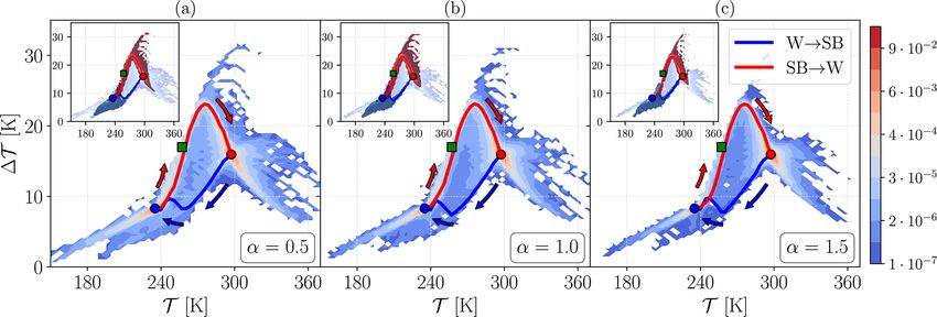
184                                                                V. Lucarini et al.: Metastability of the Ghil–Sellers model

els (EBMs), which, despite their simplicity, were able to cap-     tions for Earth-like exoplanets (see Lucarini et al., 2013, and
ture the essential physical mechanisms in action, i.e. the in-     Linsenmeier et al., 2015).
terplay between two key feedbacks. The Boltzmann feedback             Additionally, several results indicate that the phase space
is associated with the fact that warmer bodies emit more           of the climate system might well be more complex than
radiation, and it is a negative, stabilising one. Instead, the     the scenario of bistability described above. Various studies
instability of the system is due to the presence of the so-        (Lewis et al., 2007; Abbot et al., 2011; Lucarini and Bódai,
called ice–albedo feedback, whereby an increase in the ice-        2017; Margazoglou et al., 2021) performed with highly non-
covered fraction of the surface leads to a further tempera-        trivial climate models report the possible existence of addi-
ture reduction for the planet because ice efficiently reflects     tional competing states, up to a total of five (Brunetti et al.,
the incoming solar radiation. These mechanisms are active at       2019; Ragon et al., 2022). In Margazoglou et al. (2021), it is
all spatial scales, including the planetary one (see Budyko,       argued that, in fact, one can see the climate as a multistable
1969, and Sellers, 1969). Such pioneering investigations of        system where multistability is realised at different hierarchi-
the multistability of the Earth’s climate were later extended      cal levels. As an example, the tipping points (Lenton et al.,
by Ghil (1976) (see also the later analysis by Ghil and Chil-      2008; Steffen et al., 2018) that characterise the current (W)
dress, 1987), who provided a comprehensive mathematical            climate state can be seen as a manifestation of a hierarchi-
framework for the problem, based on the study of the bi-           cally lower multistability with respect to the one defining the
furcations of the system. The main control parameter defin-        dichotomy between the W and SB states.
ing the stability properties is the solar irradiance S ∗ . Below
the critical value SW→SB , only the SB state is permitted,         1.2   Transitions between competing metastable states:
whereas, above the critical value SSB→W , only the W state               Gaussian vs. Lévy noise
is permitted. Such critical values, which determine the re-
gion of bistability, are defined by bifurcations that emerge       Clearly, in the case of autonomous systems where the phase
when, roughly speaking, the strength of the positive, desta-       space is partitioned in more than one basin of attraction of
bilising feedbacks becomes as strong as the negative, stabil-      the corresponding attractors and the basin boundaries, the
ising feedbacks. Many variants of the models proposed by           asymptotic state of the system is determined by its initial
Budyko and Sellers have been discussed in the literature, all      conditions. Things change dramatically when one includes
featuring by and large rather similar qualitative and quanti-      time-dependent forcing which allows for transitions between
tative features (Ghil, 1981; North et al., 1981; North, 1990;      competing metastable states (Ashwin et al., 2012). In partic-
North and Stevens, 2006). Furthermore, these models have           ular, following the viewpoint originally proposed by Hassel-
long been receiving a great deal of attention from the math-       mann (1976), whereby the fast variables of the climate sys-
ematical community regarding the possibility of proving the        tem act as stochastic forcings for the slow ones (Imkeller and
existence of solutions and evaluating their multiplicity (Het-     von Storch, 2001), the relevance of studying noise-induced
zer, 1990; Díaz et al., 1997; Kaper and Engler, 2013; Bensid       transitions between competing states has become apparent
and Díaz, 2019).                                                   (Hänggi, 1986; Freidlin and Wentzell, 1984). This view-
   Only later were these predictions confirmed by actual           point, where the noise is usually assumed to be Gaussian
data. Indeed, geological and paleomagnetic evidence sug-           distributed, has provided very valuable insight on the mul-
gests that, during the Neoproterozoic era, between 630 × 106       tiscale nature of climatic time series (Saltzman, 2001) and is
and 715 × 106 years ago, the Earth went, at least twice, into      related to the discovery of phenomena like stochastic reso-
major long-lasting global glaciations that can be associated       nance (Benzi et al., 1981; Nicolis, 1982).
with the SB state (see Pierrehumbert et al., 2011, and Hoff-          Metastability is ubiquitous in nature, and advancing its
man et al., 1998). Multicellular life emerged in our planet        understanding is a key challenge in complex system sci-
shortly after the final deglaciation from the last SB state        ence at large (Feudel et al., 2018). In general, the transi-
(Gould, 1989). The robustness and importance of the com-           tions between competing metastable states in stochastically
petition between the Boltzmann feedback and the ice–albedo         perturbed multistable systems take place, in the weak noise
feedback in defining the global stability properties of the        limit, through special regions of the basin boundaries, which
climate has been confirmed by investigations performed us-         are named edge states. The edge states are saddles, and
ing higher complexity models (Lucarini et al., 2010; Pierre-       the trajectories initialised in the basin boundaries are at-
humbert et al., 2011), including fully coupled climate mod-        tracted to them, but there is an extra direction of instabil-
els (Voigt and Marotzke, 2010). While the mechanisms de-           ity, so that a small perturbation sends an orbit towards one
scribed above are pretty robust, the concentration of green-       of the competing metastable states with a probability of one
house gases and the boundary conditions defined by the ex-         (Grebogi et al., 1983; Ott, 2002; Kraut and Feudel, 2002;
tent and position of the continents have an impact on the          Skufca et al., 2006; Vollmer et al., 2009). In the case the
values of SW→SB and SSB→W , as well as on the properties           edge state supports chaotic dynamics, we refer to it as the
of the competing states. The presence of multistability has a      melancholia (M) state (Lucarini and Bódai, 2017). In pre-
key importance in terms of determining habitability condi-         vious papers, we have shown that it is possible to construct

Nonlin. Processes Geophys., 29, 183–205, 2022                                         https://doi.org/10.5194/npg-29-183-2022
V. Lucarini et al.: Metastability of the Ghil–Sellers model                                                                      185

M states in high-dimensional climate models (Lucarini and           ternative to the universal multifractal. Finally, we remark that
Bódai, 2017) and to prove that the nonequilibrium quasi-            fractional Fokker–Planck equations have been proposed by
potential formalism introduced by Graham (1987) and Gra-            Schertzer et al. (2001) to investigate the properties of non-
ham et al. (1991) provides a powerful framework for explain-        linear Langevin-type equations forced by an α-stable Lévy
ing the population of each metastable state and the statis-         noise with the goal of analysing and simulating anomalous
tics of the noise-induced transitions. In the weak noise limit,     diffusion.
edge states act as gateways for noise-induced transitions be-          Following Ditlevsen (1999), it has become apparent that
tween the metastable states (Lucarini and Bódai, 2019; Lu-          more general classes of α-stable Lévy noise laws might be
carini and Bódai, 2020; Margazoglou et al., 2021); see also a       useful for modelling noise-induced transitions in the cli-
recent study on a nontrivial metastable prey–predator model         mate system like Dansgaard–Oeschger events, which are se-
(Garain and Sarathi Mandal, 2022). The local minima and             quences of periods of abrupt warming followed by slower
the saddles of the quasi-potential 8, which generalises the         cooling that occurred during the last glacial period (Barker
classical energy landscape for non-gradient systems, corre-         et al., 2011). The viewpoint by Ditlevsen (1999) was particu-
spond to competing metastable states and to edge states, re-        larly effective in stimulating mathematical investigations into
spectively. In our investigation, the climate system is forced      noise-induced escapes from attractors, where, as stochastic
by adding a random – Gaussian-distributed – component to            forcing, one chooses a Lévy, rather than Gaussian, noise
the solar irradiance, which impacts, in the form of multiplica-     (Imkeller and Pavlyukevich, 2006a, b; Chechkin et al., 2007;
tive noise, only a small subset of the degrees of freedom of        Debussche et al., 2013). Such analyses have clarified that a
the system. We remark that such a choice of the stochastic          fundamental dichotomy exists with the classical Freidlin and
forcing does not fully reflect the physical realism, as the vari-   Wentzell scenario mentioned above, even if phenomena like
ability of the solar irradiance has a more complex behaviour        stochastic resonance can also be recovered in this case (Dy-
(Solanki et al., 2013). Instead, noise acts as a tool for explor-   biec and Gudowska-Nowak, 2009; Kuhwald and Pavlyuke-
ing the global stability properties of the system, and injecting    vich, 2016). Whereas, in the Gaussian case, transitions be-
noise as fluctuation of the solar irradiance has the merit of       tween competing attractors occur as a result of the very un-
impacting the Lorenz energy cycle, thus effecting all degrees       likely combination of many steps all going in the right di-
of freedom of the system (Lucarini and Bódai, 2020). See            rection, in the Lévy case, transitions result from individual,
also the recent detailed mathematical analysis of the stochas-      very large and very rare jumps. Recently, Duan and collab-
tically perturbed one-dimensional EBMs presented in Díaz            orators have made fundamental progress in achieving a vari-
and Díaz (2021).                                                    ational formulation of the Lévy noise-perturbed dynamical
   A major limitation of this mathematical framework is the         systems (Hu and Duan, 2020) and in developing correspond-
need to rigidly consider Gaussian noise laws, even if con-          ing methods for data assimilation (Gao et al., 2016) and data
siderable freedom is left as to the choice of the spatial cor-      analysis (Lu and Duan, 2020). In terms of applications, Lévy
relation properties of the noise. It seems natural to attempt       noise is becoming a more and more a popular concept and
a generalisation by considering the whole class of α-stable         tool for studying and interpreting complex systems (Grigoriu
Lévy noise laws. Lévy processes (Applebaum, 2009; Duan,             and Samorodnitsky, 2003; Penland and Sardeshmukh, 2012;
2015), described in detail in Appendix A, are fundamentally         Zheng et al., 2016; Wu et al., 2017; Serdukova et al., 2017;
characterised by the stability parameter α ∈ (0, 2], where the      Cai et al., 2017; Singla and Parthasarathy, 2020; Gottwald,
α = 2 case corresponds to the Gaussian case (which is, in-          2021).
deed, a special Lévy process). In what follows, when we dis-           The contribution by Gottwald (2021) is especially worth
cuss Lévy noise laws, we refer to α ∈ (0, 2).                       recapitulating because of its methodological clarity. There,
   Note that α-stable Lévy processes have played an impor-          the idea is, following Ditlevsen (1999), to provide a con-
tant role in geophysics as they have provided the starting          ceptual deterministic climate model able to generate a Lévy-
point for defining the multiplicative cascades also referred        noise-like signal to describe, at least qualitatively, abrupt cli-
to as universal multifractal. This framework has been pro-          mate changes similar to Dansgaard–Oeschger events. A key
posed as way to analyse and simulate, at climate scales, the        building block is the idea proposed in Thompson et al. (2017)
ubiquitous intermittency and heavy-tailed statistics of clouds      that a Lévy noise can be produced by integrating the so-
(Schertzer and Lovejoy, 1988), rain reflectivity (Tessier et al.,   called correlated additive and multiplicative (CAM) noise
1993; Schertzer and Lovejoy, 1997), atmospheric turbulence          processes, which are defined by starting from standard Gaus-
(Schmitt et al., 1996), and soil moisture (Millàn et al., 2016).    sian processes. The other key ingredient is to consider the
On longer timescales, multiplicative cascades have been             atmosphere as the fast component in the multiscale model
used to interpret temperature records in the summit ice core        and deduce, using homogenisation theory (Pavliotis and Stu-
Schmitt et al. (1995, see Lovejoy and Schertzer, 2013, for          art, 2008; Gottwald and Melbourne, 2013), that its influence
a summary of this viewpoint). Mathematicians, on the other          on the slower climate components can be closely represented
hand, have defined a Lévy multiplicative chaos (Fan, 1997;          as a Gaussian forcing. Finally, the temperature signal is cast
Rhodes et al., 2014) as a more mathematically tractable al-         as the integral of a CAM process.

https://doi.org/10.5194/npg-29-183-2022                                         Nonlin. Processes Geophys., 29, 183–205, 2022
186                                                                V. Lucarini et al.: Metastability of the Ghil–Sellers model

   We remark that Gaussian and Lévy noise can be associated        noise limit, the escapes from a given basin of attraction oc-
with stochastic forcings of a fundamentally different nature.      cur through the boundary region closest to the outgoing at-
One might think of Gaussian noise as being associated to the       tractor. Hence, the paths are very different from the Gaussian
impact of very rapid unresolved scales of motion on the re-        case (especially so for the freezing transition) and, somewhat
solved ones Pavliotis and Stuart (2008). Instead, one might        surprisingly, are identical regardless of the value of α consid-
interpret α-stable Lévy noise as describing, succinctly, the       ered. These properties can be better understood by studying
impact of what in the insurance sector are called acts of God      the impact of including singular perturbations to the value of
(e.g. an asteroid hitting the Earth, a massive volcanic erup-      the solar irradiance.
tion, or the sudden collapse of the West Antarctic ice sheet).        The rest of the paper is organised as follows. In Sect. 2,
                                                                   we present the Ghil–Sellers EBM and summarise its most
1.3   Outline of the paper and main results                        important dynamical aspects and the steady-state solutions
                                                                   and their stability. The stochastic partial differential equation
We consider here the Ghil–Sellers Earth’s EBM (Ghil, 1976),        obtained by randomly perturbing the solar irradiance in the
a diffusive, one-dimensional energy balance system, gov-           EBM is given in Sect. 3, where we also clarify the mathemat-
erned by a nonlinear reaction–diffusion parabolic partial dif-     ical meaning of the solution of the stochastic partial differen-
ferential equation. We stochastically perturb the system by        tial equation. Section 3 also introduces the mean residence
adding random fluctuations to the solar irradiance; therefore,     time and most probable transition path between the compet-
the noise is introduced in a multiplicative form. We study the     ing climate states. The numerical methods are also briefly
transitions between the two competing metastable climate           presented. In Sect. 4, we discuss our main results. In Sect. 5,
states and carry out a comparison of the effect of considering     we present our conclusions and perspectives for future inves-
Lévy vs. Gaussian noise laws of weak intensity ε.                  tigations. Finally, Appendix A presents a succinct description
   The main challenges of the problem are (a) the fact that        of α-stable Lévy processes, Appendix B sketches the deriva-
we are considering dynamical processes occurring in infinite       tion of the scaling laws for mean residence times presented in
dimensions (Doering, 1987; Duan and Wang, 2014; Alharbi,           Debussche et al. (2013), Appendix C explores the behaviour
2021) and (b) the consideration of multiplicative Lévy noise       and dynamics of singular Lévy perturbations of different du-
laws (Peszat and Zabczyk, 2007; Debussche et al., 2013). We        ration, and Appendix D presents a tabular summary of the
characterise noise-induced transitions between the compet-         statistics of the problem.
ing climate basins and quantify the effect of noise parame-
ters on them by estimating the statistics of escape times and
empirically constructing mean transition pathways called in-       2   The Ghil–Sellers energy balance climate model
stantons.
                                                                   The Ghil–Sellers EBM (Ghil, 1976) is described by a one-
   The results obtained confirm that, in the weak noise limit
                                                                   dimensional nonlinear, parabolic, reaction–diffusion partial
ε → 0, the mean residence time in each metastable state
                                                                   differential equation (PDE) involving the surface tempera-
driven by Gaussian vs. Lévy noise has a fundamentally dif-
                                                                   ture T field and the transformed space variable x = 2φ/π ∈
ferent dependence on ε. Indeed, as expected, in the Gaus-
                                                                   [−1, 1], where φ ∈ [−π/2, π/2] is the latitude. The model
sian case, the residence time grows exponentially with ε −2 ,
                                                                   describes the processes of energy input, output, and diffusion
which is, thus, in basic agreement with the well-known
                                                                   across the domain and can be written as follows:
Kramers (1940) law and the previous studies performed on
climate models (Lucarini and Bódai, 2019; Lucarini and Bó-         C(x)Tt = DI (x, T , Tx , Txx ) + DII (x, T ) − DIII (T ),    (1)
dai, 2020). Instead, in the case of α-stable noise laws, the
residence time increases with ε −α . We perform simulations        where C(x) is the effective heat capacity, and T = T (x, t)
for α = {0.5, 1.0, 1.5}. The obtained scaling can be explained     has boundary and initial conditions, as follows:
by effectively treating the Lévy noise as a compound Poisson
process, and this is in agreement with what is found for low-      Tx (−1, t) = Tx (1, t) = 0,        T (x, 0) = T0 (x).        (2)
dimensional dynamics (Imkeller and Pavlyukevich, 2006a, b)
                                                                      The equation does not depend explicitly on the time t. The
and for the infinite dimensional stochastic Chafee–Infante
                                                                   subscripts t and x refer to partial differentiation. The first
reaction–diffusion equation (Debussche et al., 2013) in the
                                                                   term – DI – on the right-hand side of Eq. (1) can be writ-
case of additive noise. This might indicate that such scaling
                                                                   ten as follows:
laws are more general than what has been so far assumed.
   Furthermore, we find clear confirmation that, in the case       DI (x, T , Tx , Txx )
of Gaussian noise in the weak noise limit, the escape from                    4
either attractor’s basin takes place through the edge state. In-   =                    [cos(π x/2)K(x, T )Tx ]x ,              (3)
                                                                       π 2 cos(π x/2)
deed, the most probable paths for both thawing and freezing
processes meet at the edge state and have distinct instantonic     and describes the convergence of meridional heat transport
and relaxation sections. In turn, for Lévy noise in the weak       performed by the geophysical fluids. The function K(x, T )

Nonlin. Processes Geophys., 29, 183–205, 2022                                              https://doi.org/10.5194/npg-29-183-2022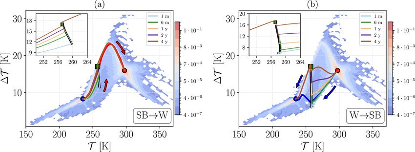
V. Lucarini et al.: Metastability of the Ghil–Sellers model 187
is a combined diffusion coefficient, expressed as follows: where slightly different parameterisations for the diffusion
operator, for the albedo, and for the greenhouse effect are
K(x, T ) = k1 (x) + k2 (x)g(T ), with (4) introduced. Such models are in fundamental agreement, both
c4 c
5 in terms of physical (Ghil, 1981; North et al., 1981; North,
g(T ) = 2 exp − . (5)
T T 1990; North and Stevens, 2006) and mathematical properties
(Hetzer, 1990; Díaz et al., 1997; Kaper and Engler, 2013;
The empirical functions k1 (x) and k2 (x) are eddy diffu-
Bensid and Díaz, 2019).
sivities for sensible and latent heat, respectively, and g(T ) is
In this study, we consider µ = 1.05. For this value of µ,
associated with the Clausius–Clapeyron relation, which de-
two stable asymptotic states – the W and the SB states – co-
scribes the relationship between temperature and saturation
exist (see Fig. 1b). Indeed, a codimension of one manifold
water vapour content of the atmosphere.
separates the basins of attraction of the W and SB states.
The second term – DII – on the right-hand side of Eq. (1)
We refer to D W (D SB ) as the basin of attraction of the W
describes the energy input associated with the absorption of
(SB state). We refer to B as the basin boundary, which in-
incoming solar radiation and can be written as follows:
cludes a single edge state M. Therefore, the system has three
DII (x, T ) = µQ(x) [1 − αa (x, T )] , (6) stationary solutions TW (x), TSB (x), and TM (x) for the W, SB,
and M state, respectively, as shown in Fig. 1a. In Ghil (1976),
where Q(x) is the incoming solar radiation, and αa (x, T ) is the three stationary solutions were obtained by equating Tt
the surface reflectivity (albedo), which is expressed as fol- to 0, and it was shown, through linear stability analysis, that
lows: the stationary solutions TW and TSB are stable, while TM is
unstable. In Bódai et al. (2015) the unstable solution TM was
αa (x, T ) = {b(x) − c1 (Tm + min [T − c2 z(x) − Tm , 0])}c , (7) constructed using a modified version of the edge-tracking al-
gorithm (Skufca et al., 2006).
where the subscript {·}c denotes a cutoff for a generic quan- Following previous studies (Bódai et al., 2015; Lucarini
tity h, defined as follows: and Bódai, 2019; Lucarini and Bódai, 2020; Margazoglou
et al., 2021), when visualising our results, we apply a coarse
hmin h ≤ hmin ,
graining to the phase space of the model. In what follows,
hc = h hmin < h < hmax , (8) we perform a projection on the plane spanned by the spa-
tially averaged temperature T and the averaged Equator mi-
hmax hmax ≤ h.
nus the poles’ temperature difference 1T , which is defined
The term c2 z(x) in Eq. (7) indicates the difference between as follows:
the sea level and surface level temperatures, and b(x) is a
temperature independent empirical function of the albedo. T = [T (x, t)]10 , (10)
The parameterisation given in Eqs. (7)–(8) encodes the pos- 1/3
itive ice–albedo feedback. The relative intensity of the solar 1T = [T (x, t)]0 − [T (x, t)]11/3 , where (11)
R xh
radiation in the model can be controlled by the parameter µ. x cos(π x/2)T (x, t)dx
xh
The last term – DIII – on the right-hand side of Eq. (1) [T (x, t)]xl = l R xh . (12)
describes the energy loss to space by outgoing thermal plan- xl cos(π x/2)dx
etary radiation and is responsible for the negative Boltzmann
feedback. It can be written as follows: Such a representation allows for a minimal yet still phys-
h i ically relevant description of the system. Indeed, changes
DIII (T ) = σ T 4 1 − m tanh(c3 T 6 ) , (9) in the energy budget of the system (warming versus cool-
ing) are, to a first approximation, related to variations in
where σ is the Stefan–Boltzmann constant, and the T , while the large-scale energy transport performed by the
emissivity coefficient is expressed as 1 − m tanh(c3 T 6 ). geophysical fluids is controlled by 1T . The boundary be-
Such a term describes, in a simple yet effective way, tween high and low latitude in Eq. (11) is established at
the greenhouse effect by reducing infrared radia- x = ±1/3, i.e. at 30◦ N/S. Additionally, in some visualisa-
tion losses. The values of the empirical functions tions, we consider, as a third coordinate, the fraction of the
C(x), Q(x), b(x), z(x), k1 (x), k2 (x) at discrete latitudes surface with a below-freezing temperature (therefore, we ex-
and empirical parameters c1 , c2 , c3 , c4 , c5 , σ, m, Tm are pect 1 for global glaciation and 0 for no ice). We refer to this
taken from Ghil (1976), as modified in Bódai et al. (2015). variable as I , and it is an attempt to extract an observable that
The choice of the empirical functions and parameters are resembles the sea ice percentage of the Earth’s surface. Thus,
extensively discussed in Ghil (1976). Of course, one might the stationary solutions TW (x), TSB (x), and TM (x), in terms
reasonably wonder about the robustness of our modelling of 1T and T , correspond to 1TW = 16 K, 1TSB = 8.3 K,
strategy. Indeed, a plethora of EBMs analogous to the 1TM = 17.5 K, T W = 297.7 K, T SB = 235.1 K, T M = 258 K,
one described here have been presented in the literature, IW = 0.2, ISB = 1, and IM = 1.
https://doi.org/10.5194/npg-29-183-2022 Nonlin. Processes Geophys., 29, 183–205, 2022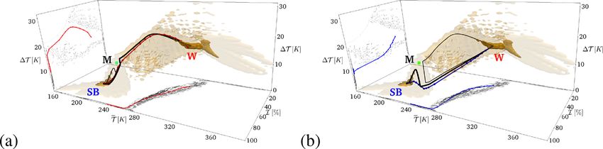
188                                                                    V. Lucarini et al.: Metastability of the Ghil–Sellers model

Figure 1. (a) Stationary solutions TW (x), TSB (x), and TM (x) in Kelvins (K) of the zonally averaged energy balance model Eq. (1). (b) Bi-
furcation diagram of the average temperature T as a function of control parameter µ.

3     Background and methodology                                        and H (k · k, h·, ·i) a separable Hilbert space with a norm k · k
                                                                        and inner product h·, ·i. Equation (13) can be rewritten in the
3.1    Stochastic energy balance model                                  more general form, as follows:
In order to analyse the influence of random perturbations on            Tt = A(x) [E(x, T ) Tx ]x + F (x, T ) + εG(x, T )L̇α (t),
the deterministic dynamics of the climate model described               Tx (−1, t) = Tx (1, t) = 0,
in Sect. 2, we perturb the relative intensity µ of the solar
irradiance by including a symmetric α-stable Lévy process               T (x, 0) = T0 (x),                                            (14)
and rewrite Eq. (1) in the form of the following stochastic
                                                                        where A, E, F, G are Lipschitz functions defined on
partial differential equation (SPDE):
                                                                        [−1, 1] × H and G(x, T )L̇α (t) = L̇(t). Under certain as-
C(x)Tt = DI (x, T , Tx , Txx )                                          sumptions (Yagi, 2010), the problem (Eq. 14) is formulated
            + DII (x, T ) 1 + ε/µL̇α (t) − DIII (T ),

                                                              (13)      as a Cauchy problem, for which a local mild solution, a pro-
                                                                        gressively measurable process T (t), for all t ∈ [0, tF ] and
where the boundary and initial conditions defined by Eq. (2)            T0 ∈ H has the following integral representation:
apply to the stochastic temperature field T . Here the param-
eter ε > 0 controls the noise intensity, and (Lα (t)t≥0 ) is a                               Zt
symmetric α-stable process defined in Appendix A. We con-               T (t) = 9(t)T0 +          9(t − s)ϒ(T (s))ds
sider symmetric processes because we want to have a sim-
                                                                                             0
ple mathematical model allowing for transitions in both the
                                                                                     Zt
SB → W and the W direction → SB direction. Instead, a
strongly skewed process would have made it very hard to ex-                     +ε        9(t − s)G(T (s))dβ
plore the full phase space because a lack of symmetry would                          0
invariably favour one of the two transitions. As mentioned                           Zt
before, we refer to the Lévy case if the stability parameter                    +ε        9(t − s)G(T (s))dγ ,                        (15)
α ∈ (0, 2), so that we consider a jump process. We recall that
                                                                                     0
the jumps become more frequent and less intense as α in-
creases.                                                                where the dependence on x is kept implicit, and β (γ ) is
   We define L̇(t) = Q(x)[1 − αa (x, T )]L̇α (t), as the gen-           the Poisson random measure (compensated Poisson random
eralised derivative of a stochastic process in a suitably de-           measure) defined through Lévy–Itô decomposition. Instead,
fined functional space. Equation (13) features multiplicative           9(t) with t>0 is the evolution operator having the gener-
noise. The research interest on this type of SPDE (Doering,             alised semigroup property for the family of sector operators
1987; Peszat and Zabczyk, 2007; Duan and Wang, 2014;                    with the bounded inverses, and ϒ(T ) = T +F (x, T ), T ∈ H
Alharbi, 2021) is mainly focused on defining weak, strong,              is a nonlinear operator, which we assume to be Lipschitz
mild, and martingale solutions, in specifying under which               continuous. Following the abstract theory presented in Yagi
conditions these solutions exist and are unique, and in con-            (2010), under certain structural assumptions for the operators
structing numerical approximation schemes for the solutions             9 and ϒ and for the functional space, one can prove that the
(Davie and Gaines, 2000; Cialenco et al., 2012; Burrage and             solution Eq. (15) is the unique local mild solution of Eq. (14).
Lythe, 2014; Jentzen and Kloeden, 2009; Kloeden and Shott,                 As mentioned above, things are radically different for the
2001), among other aspects.                                             special case α = 2, which corresponds to Gaussian noise.
   First, let us define the concept of a mild solution in this          In this case, we revisit Eq. (14), and we define L̇α=2 (t) =
context. Let (, F, P) be a given complete probability space            Ẇ (t), where (W (t)t≥0 ) is a Wiener process. We then de-

Nonlin. Processes Geophys., 29, 183–205, 2022                                                https://doi.org/10.5194/npg-29-183-2022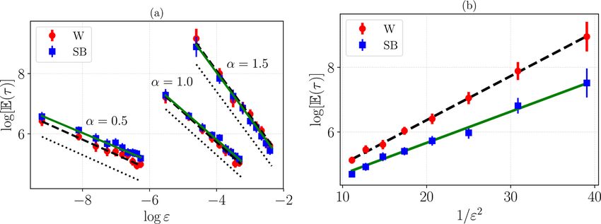
V. Lucarini et al.: Metastability of the Ghil–Sellers model                                                                       189

fine Ẇ(t) = G(x, T )Ẇ (t) as the generalised derivative of a       not actually play any relevant role in determining the tran-
Wiener process in a suitably defined functional space.               sitions, while they are responsible for the variability within
                                                                     each basin of attraction.
3.2   Noise-induced transitions: mean escape times                      We now consider the case α = 2. While the correspond-
                                                                     ing finite dimensional problem is thoroughly documented in
By incorporating stochastic forcing into the system, its long-       the literature (Freidlin and Wentzell, 1984) and has been ap-
time dynamics change significantly, allowing transitions be-         plied in a similar context by some of the authors (Lucarini
tween the competing basins. This dynamical behaviour is              and Bódai, 2019; Lucarini and Bódai, 2020; Ghil and Lu-
called metastability and is graphically captured by Fig. 2,          carini, 2020; Margazoglou et al., 2021), the treatment of in-
where, in Fig. 2a and b, a typical spatiotemporal evolution          finite dimensional SDEs driven by an infinite dimensional
of the temperature field is shown for the stability parameters       Wiener process via the Freidlin–Wentzell theory requires fur-
α = 0.5 and α = 1.5, respectively. Instead, in Fig. 2c and d,        ther extension. In the present context, we refer to Budhiraja
the temporal evolution of the global temperature T and of            and Dupuis (2000) and Budhiraja et al. (2008) and refer-
the averaged Equator and poles’ temperature difference 1T            ences therein, where the problem of an infinite dimensional
(as defined in Eqs. 10–11) is correspondingly shown. In what         reaction–diffusion equation driven by an infinite dimensional
follows, we investigate the time statistics and the paths of the     Wiener process has been addressed.
transitions between such basins.                                        We assume that steady-state conditions and ergodicity are
   In a complete probability space (, F, P) we define the           met, and we also assume that the analysing system is bistable
first exit time τx of a cádlág mild solution T (·; x) of Eq. (13),   and a unique edge state is present at the basin boundary, as
starting at the x ∈ D W/SB domain of a W/SB climate stable           in the case studied here. In the case of Gaussian noise, tran-
state as follows:                                                    sitions between the competing basins of attraction are not
            n                          o                             determined by a single event as in the 0 < α < 2 case but,
τx (ω) = inf t > 0|Tt (ω, x) 6 ∈ D W/SB ,   ω ∈ , x ∈ H.    (16)    instead, occur as a result of very unlikely combinations of
                                                                     subsequent realisations of the stochastic variable acting as a
   The mean escape time is then expressed by E[τx (ω)]. In           forcing. In the weak noise limit, the transitions occur accord-
the case of the infinite dimensional multistable reaction–           ing to the least unlikely (yet very unlikely) chain of events,
diffusion system described by Chafee–Infante equation un-            whose probability is described using a large deviation law
der the influence of additive infinite-dimensional α-stable          (Varadhan et al., 1985). One finds that the mean escape time
Lévy noise – α ∈ (0, 2) – it was shown (Debussche et al.,            from either basin of attraction decreases exponentially with
2013) that, in the weak noise limit, ε → 0 the mean es-              increasing noise intensity ε and is given by a generalised
cape time from one of the competing basins of attraction             Kramers’ law, as follows:
increases as ε −α . In such a limit, the jump diffusion sys-
                                                                                             218W→M/SB→M (T )
tem reduces the Markov chain to a finite state, with val-            E[τW/SB (ε)] ≈ exp                               ,         (17)
ues in the set of stable states. Details of this method are                                           ε2
given in Appendix B. Similar results have been obtained              where 18W→M = 8M (T ) − 8W (T ) is the height of the
for bistable one-dimensional stochastic differential equations       quasi-potential barrier in the W attractor; correspondingly,
(SDEs; Imkeller and Pavlyukevich, 2006a, b). The basic rea-          18SB→M (T ) = 8M (T )−8SB (T ) is the height of the quasi-
son behind this result is that, in order to study the transitions    potential barrier in the SB attractor, and 8 is the Graham
between the competing basins of attraction, one can treat the        quasi-potential mentioned above (Graham, 1987; Graham
Lévy noise as a compound Poisson process, where jumps ar-            et al., 1991).
rive randomly, according to a Poisson process, and the size
of the jumps x is given by a stochastic process that obeys a         3.3   Noise-induced transitions: most probable
specified probability distribution. For a symmetric α-stable               transition paths
Lévy process, such a distribution asymptotically decreases
as |x|−1−α , as discussed in Appendix A. Let us assume that          In the weak noise limit, the most probable path to escape an
positive values of x bring the state of the system closer to         attractor is defined by a class of trajectories named instantons
the basin boundary (as in the case of positive fluctuations          (Grafke et al., 2015, 2017; Bouchet et al., 2016; Grafke and
of the solar irradiance when studying escapes from the SB            Vanden-Eijnden, 2019) or maximum likelihood escape paths
state). Assuming a simple geometry for the basin boundary,           (Lu and Duan, 2020; Dai et al., 2020; Hu and Duan, 2020;
we find that a transition takes place when an event larger than      Zheng et al., 2020). However, note that different noise laws
a critical value xcrit > 0 is realised. The probability of such      result into possibly radically different instantonic trajectories
                         −α
an event scales with xcrit  . A similar argument applies when        (Dai et al., 2020; Zheng et al., 2020).
considering transitions triggered by negative fluctuations of           In our case, the theory indicates that, if the stochastic forc-
the stochastic variable. Small-size events, which occur fre-         ing is Gaussian, under a rather general hypothesis, the in-
quently and correspond to the non-occurrence of jumps, do            stanton will connect the attractor W/SB with the edge state

https://doi.org/10.5194/npg-29-183-2022                                          Nonlin. Processes Geophys., 29, 183–205, 2022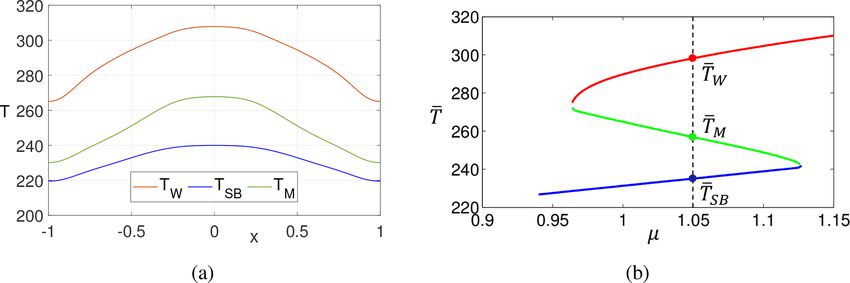
190                                                                      V. Lucarini et al.: Metastability of the Ghil–Sellers model

M, which then acts as gateway for noise-induced transi-                     The time span of integration t ∈ [0, Tf ], varies for differ-
tions. Once the quasi-potential barrier is overcome, a free-             ent cases, with Tf ∈ (105 , 15 × 105 ) years, with a time step-
fall relaxation trajectory links M with the competing at-                ping of 1 year. Each year, we consider a different value for the
tractor SB/W. For equilibrium systems, (e.g. for gradient                relative solar irradiance by extracting a random number Zj
flows), where a detailed balance is achieved, the relaxation             (see Eq. 19). To simulate the stochastic noise term εLα (t),
and instantonic trajectories within the same basin of attrac-            which is added in the parameter µ in Eq. (13), we use the
tion are identical. On the contrary, for non-equilibrium sys-            recursive algorithm from Duan (2015). The process values
tems, the relaxation and instantonic trajectories will differ            Lα (t1 ), . . ., Lα (tN ) at each moment tj , j ∈ N are obtained via
and will only meet at the attractor. (See a detailed discus-             the following:
sion of this aspect and of the dynamical interpretation of the                                                  1
quasi-potential 8 in Lucarini and Bódai, 2020, and Marga-                Lα (tj ) = Lα (tj −1 ) + (tj − tj −1 ) α Zj ,   j = 1, . . ., N, (19)
zoglou et al., 2021). Instead, if the noise is of Lévy type, the         where the second term is an independent increment, and
theory formulated for simpler equations suggests that the in-            Zj are the independent standard symmetric α-stable random
stanton will connect the attractor with a region on the basin            numbers generated by an algorithm in Weron and Weron
boundary that is the nearest, in the phase space, to the at-             (1995, see also Grafke et al., 2015, for a detailed explana-
tractor, as the concept of the quasi-potential is immaterial             tion of the steps above). For illustrative reasons, some sam-
(Imkeller and Pavlyukevich, 2006a, b).                                   ple solutions of Eq. (13) for different values of α are shown
   In general, the maximum likelihood transition trajectory              in Fig. 2a and b.
TM (t) can be defined (Zheng et al., 2020; Lu and Duan, 2020)               For the numerical simulations discussed below, we con-
as a set of system states at each time moment t ∈ [0, tf ]               sider α = (0.5, 1.0, 1.5, 2) and ε ∈ (0.0001, 0.3). We select ε
that maximises the conditional probability density function              in such a way that the noise intensity is strong enough to in-
p( . | . ; . ) of the passage from the origin stable state               duce at least an order of 10 transition, given our constraints
φ W/SB to the destination stable state φ SB/W and is expressed           in the time length of the simulations, and weak enough that
as follows:                                                              we are not far from the weak noise limit, where the scal-
TM (t)                                                                   ing laws discussed above apply and transitions paths are well
                                                                       organised. Our simulations are performed by taking the Itô
= arg max        p (T (t) = x | T (0) = x0 ; T (tf ) = xf )
         x                                                               interpretation for the stochastic equations.
                                                                            We remark that, when we consider Lévy noise, it does hap-

  p T (tf ) = xf | T (t) = x · p (T (t) = x | T (0) = x0 )
=                                                          ,      (18)   pen that, for some years, the solar irradiance has negative val-
               p (T (tf ) = xf | T (0) = x0 )
                                                                         ues. Of course these conditions bear no physical relevance,
where x0 (xf ) belongs to the basin of attraction D W/SB                 and are a necessary result of considering unbounded noise.
(D SB/W ), and p ( . | . ) is the probability density function           Nonetheless, we have allowed for this to occur in our simu-
evolving according to the Fokker–Planck equation (Risken,                lations in order to be able to stick to the desired mathemat-
1996). This method is applicable either if efficient numerical           ical framework. We remind the reader that this study does
algorithms are available to solve the Fokker–Planck equation             not aim at capturing, with any high degree of realism, the de-
associated to the studied stochastically driven system, or, em-          scription of the actual evolution of climate. At any rate, as
pirically, when considering a large ensemble of simulations.             can be understood from the discussion below in Sect. 4.2.2
Note that this is not an asymptotic approach, i.e. it does not           and from what is reported in Appendix C, were we to con-
require a weak noise limit ε → 0 and is applicable for sys-              sider longer-lasting (e.g. 2 years vs. 1 year) fluctuations of the
tems with either Gaussian or non-Gaussian noise. Yet, in the             solar irradiance, a satisfactory exploration of the transitions
weak noise limit, the definition (Eq. 18) leads to constructing          between the competing W and SB states would be possible
the optimal transition paths described above.                            with a greatly reduced occurrence of such unphysical events,
   In the following section, for practical purposes, we con-             and the basic reason for this being the presence of a larger
                                                                                              1
struct such optimal transition path in the coarse-grained 2D             factor (tj − tj −1 ) α in Eq. (19).
phase space (T , 1T ) and 3D phase space (T , 1T , I) of the
variables defined in Sect. 2 by averaging the ensemble of
transitions connecting the two competing states in the weak              4   Results and discussion
noise limit.
                                                                         In what follows, we aim at addressing three main ques-
3.4   Numerical methods                                                  tions: (1) what are the temporal statistics of the SB → W
                                                                         and W → SB transitions? (2) What are the typical transition
We solve Eq. (13) through the MATLAB pdepe function,                     pathways? (3) What are the fundamental differences between
which is well suited for solving 1D parabolic and elliptic               transitions caused by Gaussian vs. Lévy noise? A summary
PDEs. We discretise the 1D space with a regular grid of 201              of the results of the numerical simulations is given in Ta-
grid points, following Bódai et al. (2015).                              ble D1 in Appendix D, including the sample size, i.e. number

Nonlin. Processes Geophys., 29, 183–205, 2022                                                 https://doi.org/10.5194/npg-29-183-2022
V. Lucarini et al.: Metastability of the Ghil–Sellers model 191
Figure 2. The metastable behaviour of the solution path of a stochastic energy balance model (Eq. 13), for ε = 0.04, T0 = 300 K, and
t ∈ (0, 300) years, for (a) α = 0.5, (b) α = 1.5, and the (c) temperature average T and (d) temperature contrast at low and high latitudes. 1T ,
for ε = 0.01, α = 0.5,andα = 1.5. Red, green, or blue dash-dotted lines portray the stationary climate states of T W /T M /T SB , respectively.
of transitions, point estimates for mean escape time, and their possibility that the ε −α scaling might apply in more general
0.95 confidence intervals for exits from both the W and SB conditions than what has been, as of yet, rigorously proven,
basins. See the data availability section for information on and this is specifically the case when multiplicative Lévy
how to access the supplement (Lucarini et al., 2022), which noise is considered. The stochastically perturbed trajectories
contains the raw data produced in this study and some illus- forced by Lévy noise consist of jumps, and the probability
trative animations portraying noise-induced transitions be- of occurrence of a high jump, which can trigger the escape
tween the two competing metastable states. from the reference basin of attraction, is polynomially small
in noise intensity ε.
4.1 Mean escape time The Gaussian case – where no jumps are present – is por-
trayed in Fig. 3b. We show, in semi-logarithmic scale, the
Our analysis confirms that there is a fundamental dichotomy mean residence time versus 1/ε2 . We perform a successful
in the statistics of mean escape times between Lévy noise linear fit of the logarithm of the mean residence time in either
and Gaussian noise-induced transitions. attractor versus 1/ε 2 , and using Eq. (17), we obtain an esti-
Figure 3a shows the dependence of the mean escape time mate of the local quasi-potential barrier 18W/SB→M , which
from either attractor on ε and α for the Lévy case. The red is half of the slope of the corresponding straight lines of the
circles (blue squares) correspond to escapes from the W (SB) linear fit (see the last column of Table 1). We conclude that,
basin (see Lucarini et al., 2022, for additional details). The for µ = 1.05, the local minimum of 8 corresponding to the
scaling ∝ ε −α presented in Eq. (B6) is shown by the dot- W state is deeper than the one corresponding to the SB state.
ted black line for each value of α. We also portray the best
power law fit of the mean residence time with respect to ε
4.2 Escape paths for the noise-induced transitions
for each value of α; the confidence intervals of the exponent
are shown in Table 1. Our empirical results seem to indicate,
at least in this case, an agreement with the ε −α scaling pre- We now explore the geometry of the transition paths asso-
sented and discussed earlier in the paper. This points at the ciated with the metastable behaviour of the system. We first
https://doi.org/10.5194/npg-29-183-2022 Nonlin. Processes Geophys., 29, 183–205, 2022192 V. Lucarini et al.: Metastability of the Ghil–Sellers model
Figure 3. Estimates of the mean escape time E(τ ) (in years) from the W (blue circles) and SB (red squares) states, as a function of the noise
intensity ε. (a) Lévy noise for α = 0.5, 1.0, and 1.5, with the dotted line being the corresponding prediction from Eq. (B6), while the straight
green (SB) and dashed black (W) lines are the fittings of Eq. (B6) of the relevant dataset. (b) Gaussian noise, with straight green (SB) and
dashed black (W) lines being the fit of Eq. (17), is shown.
Table 1. Estimates of the exponent α via the fitting of Eq. (B6) sponds to the SB (W) state and of the M state (green square).
for the Lévy case (three first columns) and of the energy barrier In the inset of Fig. 4a, we present the ensemble of W → SB
18W/SB→M via the fitting of Eq. (17) for the Gaussian case (last (SB → W) transitions as deep blue (red) contours. The most
column). In parenthesis, the estimated error of the last digit is probable transition paths are shown in blue for the W → SB
shown. and in red for the SB → W. The instantonic portion of the
blue (red) line is the one connecting the W (SB) attractor to
Lévy Gaussian
the M state and is portrayed as a solid line, while the relax-
α 0.5 1.0 1.5 2 ation portion, connecting the M state with the SB (W) at-
W 0.50(2) 1.00(2) 1.50(1) 18W→M = 0.068(1) tractor, is portrayed as a dashed line. Within each basin of
SB 0.47(2) 0.97(2) 1.52(4) 18SB→M = 0.048(3) attraction, the instantonic and relaxation trajectories do not
coincide, and, instead, only meet at the corresponding attrac-
tor and at the M state. This is particularly clear for the W
discuss the case of Gaussian noise because it is indeed more state. The presence of such a loop, proving the existence of
familiar and more extensively studied. non-vanishing probability currents and the breakdown of de-
tailed balance, is a signature of non-equilibrium dynamics,
4.2.1 Gaussian noise which was also observed in Margazoglou et al. (2021) and
has, instead, gone undetected in Lucarini and Bódai (2019)
We estimate the transition paths by averaging among the and Lucarini and Bódai (2020). See Lucarini et al. (2022) for
escape plus relaxation trajectories using the run performed some illustrative simulations of the transitions.
with the weakest noise (see Table D1). We first perform our Let us provide some physical interpretation of how the
analysis in the 2D-projected state space defined by (T , 1T ). transitions occur. Looking at the SB → W most probable
We prescribe two small circular-shaped regions enclosing the path, the escape includes a simultaneous increase in T and
two deterministic attractors and search the time series of the 1T . In practice, a SB → W transition takes place when,
portions of the whole trajectory that leave one of these re- starting at the SB state, one has a (rare) sequence of positive
gions and reach the other one. This creates two subsets of our anomalies in the fluctuating solar irradiance e µ, i.e. e
µ > µ.
full dataset from which we build a 2D histogram for each of While the planet is warming globally, the Equator is warm-
the SB → W and W → SB transitions in the projected space. ing faster than the poles, resulting in a positive rate 1T˙ > 0,
We then estimate the most probable transition paths by find- because it receives, in relative and absolute terms, more in-
ing, for each bin value of T , the peak of the histogram in the coming solar radiation. Considering that the Equator also in
1T direction. The distributions are very peaked, and almost the SB state is warmer than the poles, the melting of the ice
indistinguishable estimates for the instantonic and relaxation conducive to the transition occurs first at the Equator, with
trajectories are obtained when computing the average of 1T a subsequent decrease in the albedo in low latitudes. Once
according to the 2D histogram conditional on the value of T . the system crosses the M state, and supposing that persistent
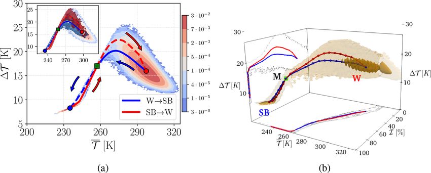
In the background of Fig. 4a, we show the empirical esti- µ < µ do not appear at this stage, the system will relax to-
e
mate of the invariant measure in the 2D-projected state space wards the W state. The relaxation includes a consistent global
defined by (T , 1T ). Additionally, we indicate the position of warming of the planet but with a change in sign in the rate
the deterministic attractors, where the blue (red) circle corre-
Nonlin. Processes Geophys., 29, 183–205, 2022 https://doi.org/10.5194/npg-29-183-2022V. Lucarini et al.: Metastability of the Ghil–Sellers model 193
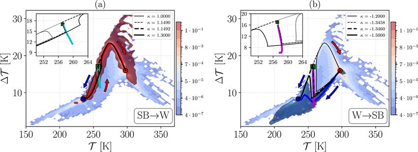
Figure 4. (a) Invariant measure in the 2D-projected state space defined by T , 1T . The coloured points indicate the deterministic attractors
of the SB (blue), M (green), and W (red) states, and the blue (red) line is the stochastically averaged transition paths for the W → SB
(SB → W) transitions. Dashed (solid) lines are the relaxation (instantonic) trajectories. The arrows show the direction of transitions. The top
left inset shows that the dark blue (red) contours portray the ensembles of the transition paths between W → SB (SB → W). Here, the system
is driven by Gaussian noise with ε = 0.14. (b) The invariant measure and most probable transition paths (W → SB in blue and SB → W
in red) in the 3D-projected state space are defined by T , 1T , I . The darker brown shading indicates a higher probability density for the
corresponding isosurface. The 2D projections on the T , I , and (1T , I) planes are shown. The location of the M state is given by a pink
square. Here, the system is driven by Gaussian noise, with ε = 0.16.
of 1T˙ , and a subsequent decrease in 1T , implying that as cross in the 3D projection in a well-defined region, which
soon as the temperature at the Equator has risen enough, the indeed corresponds to the M state (pink square).
poles will then warm at a faster pace because the ice–albedo
effect kicks in. 4.2.2 Lévy noise
The global freezing of the planet associated with the W →
SB transition is qualitatively similar but not identical to the There is scarcity of rigorous mathematical results regarding
reverse SB → W process. Notice a considerable overlap of the weak noise limit of the transition paths between compet-
the transition paths ensembles in both basins of attraction, ing states in metastable stochastic systems forced by multi-
shown as red and blue contours in the inset of Fig. 4a. This plicative Lévy noise. Indeed, the derivation of analytical re-
implies the presence of less extreme non-equilibrium condi- sults for this type of system largely remains an open problem.
tions compared to what was observed in Margazoglou et al. Recently, for stochastic partial differential equations with ad-
(2021), where the W → SB and SB → W transitions oc- ditive Lévy and Gaussian noise, the Onsager–Machlup action
curred through fundamentally different paths (see the discus- functional has been derived in Hu and Duan (2020), lead-
sion therein, especially regarding the role of the hydrological ing to a precise formulation of the most probable transition
cycle). paths. Hence, we do not have solid mathematical results to
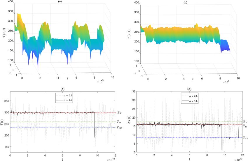
Figure 4b presents the optimal transition paths W → SB interpret what we describe below, where, instead, we need to
and SB → W in a three-dimensional projection, where we use heuristic arguments. As far as we know, this is the first
add, as a third coordinate, the variable I, which indicates attempt to estimate the most probable transition pathway be-
the fraction of the surface that has subfreezing tempera- tween the metastable states in infinite stochastic systems with
tures (T < 273.15 K). On the sides of the figure, two two- multiplicative pure Lévy process.
dimensional projections on the (T , 1I) and on the (1T , I) A striking feature in Fig. 5 is that the invariant measure and
planes are shown. Here, darker brown shadings indicate the the structure of the most probable transition paths (SB → W
higher density of points and the red and blue dots sample and W → SB), in the weak noise limit, are fundamentally
the highest probability for the SB → W and W → SB tran- different between the Lévy case and the Gaussian one. The
sitions paths, respectively. One could argue that the presence invariant measure is highly peaked (dark red in the colour
of an intersection between the SB → W and W → SB high- scheme) in a small region around the deterministic attrac-
est probability transition paths in Fig. 4a could have been a tors, as, most typically, the Lévy noise fluctuations of e µ are
simple effect of 2D projection. Instead, we see here that the very small. Additionally, the most probable transition paths
SB → W and W → SB most probable transition paths also depend very weakly on the chosen value for the stability pa-
rameter α. This suggests that the geometry of most proba-
ble path of transitions does not depend on the frequency and
https://doi.org/10.5194/npg-29-183-2022 Nonlin. Processes Geophys., 29, 183–205, 2022You can also read