Linking plant and soil indices for water stress management in black gram
←
→
Page content transcription
If your browser does not render page correctly, please read the page content below
www.nature.com/scientificreports
OPEN Linking plant and soil indices
for water stress management
in black gram
Afshin Khorsand1, Vahid Rezaverdinejad2*, Hossein Asgarzadeh3, Abolfazl Majnooni‑Heris4,
Amir Rahimi5, Sina Besharat1 & Ali Ashraf Sadraddini4
Measurement of plant and soil indices as well as their combinations are generally used for irrigation
scheduling and water stress management of crops and horticulture. Rapid and accurate determination
of irrigation time is one of the most important issues of sustainable water management in order to
prevent plant water stress. The objectives of this study are to develop baselines and provide irrigation
scheduling relationships during different stages of black gram growth, determine the critical limits
of plant and soil indices, and also determine the relationships between plant physiology and soil
indices. This study was conducted in a randomized complete block design at the four irrigation
levels 50 (I1), 75 (I2), 100 (I3 or non-stress treatment) and 125 (I4) percent of crop’s water requirement
with three replications in Urmia region in Iran in order to irrigation scheduling of black gram using
indices such as canopy temperature (Tc), crop water stress index (CWSI), relative water content
(RWC), leaf water potential (LWP), soil water (SW) and penetration resistance (Q) of soil under one-
row drip irrigation. The plant irrigation scheduling was performed by using the experimental crop
water stress index (CWSI) method. The upper and lower baseline equations as well as CWSI were
calculated for the three treatments of I1, I2 and I3 during the plant growth period. Using the extracted
baselines, the mean CWSI values for the three treatments of I1, I2 and I3 were calculated to be 0.37,
0.23 and 0.15, respectively, during the growth season. Finally, using CWSI, the necessary equations
were provided to determine the irrigation schedule for the four growing stages of black gram,
i.e. floral induction-flowering, pod formation, seed and pod filling and physiological maturity, as
(Tc − Ta)c = 1.9498 − 0.1579(AVPD), (Tc − Ta)c = 4.4395 − 0.1585(AVPD), (Tc − Ta)c = 2.4676 − 0.0578(AVPD)
and (Tc − Ta)c = 5.7532 − 0.1462(AVPD), respectively. In this study, soil and crop indices, which were
measured simultaneously at maximum stress time, were used as a complementary index to remove
CWSI constraints. It should be noted that in Urmia, the critical difference between the canopy
temperature and air temperature (Tc − Ta), soil penetration resistance (Q), soil water (SW) and relative
water content (RWC) for the whole growth period of black gram were − 0.036 °C, 10.43 MPa and
0.14 cm3 cm−3 and 0.76, respectively. Ideal point error (IPE) was also used to estimate RWC, (Tc − Ta)
and LWP as well as to select the best regression model. According to the results, black gram would
reduce its RWC less through reducing its transpiration and water management. Therefore, it can be
used as a low-water-consuming crop. Furthermore, in light of available facilities, the farmer can use
the regression equations between the obtained soil and plant indices and the critical boundaries for
the irrigation scheduling of the field.
Abbreviations
AVPD Air vapor pressure deficit (mbar)
AVPG Air vapor pressure gradient (mbar)
a and b Intercept a and slope b are the linear regression parameters of ( Tc − Ta)L.L on AVPD (–)
BD Bulk density (g c m−3)
CWSI Crop water stress index (–)
DW Weight of leaf dried in oven (g)
1
Department of Water Engineering, Urmia University, Urmia, Iran. 2Department of Water Engineering, Urmia
University, 11 Km Sero Road, Post box: 165, 5756151818 Urmia, Iran. 3Department of Soil Science, Urmia
University, Urmia, Iran. 4Department of Water Engineering, University of Tabriz, Tabriz, Iran. 5Department of
Agronomy, Urmia University, Urmia, Iran. *email: v.verdinejad@urmia.ac.ir
Scientific Reports | (2021) 11:869 | https://doi.org/10.1038/s41598-020-79516-3 1
Vol.:(0123456789)www.nature.com/scientificreports/
es(Ta) Air vapor pressure at Ta (mbar)
ETc Crop evapotranspiration (mm)
ETo Reference evapotranspiration (mm)
FC Field capacity (cm3 cm−3)
FW Fresh leaf weight (g)
h Soil matric suction (hPa)
IPE Ideal point error (–)
IRT Infrared thermometer (°C)
Kc Crop coefficient (–)
LWP Leaf water potential (bar, MPa)
MAE Mean absolute error ((–), °C, bar)
MRE Mean relative error (–)
n Pore size distribution index (–)
N Number of measurements (instances) (–)
Oi and Pi Observed and predicted values (–)
Oi and Pi Mean of the observed and predicted values (–)
PR2 Profile probe (V%)
PWP Permanent wilting point (cm3 cm−3)
Q Penetration resistance (MPa)
Qh Maximum (dry) predicted soil penetration resistance (MPa)
Ql Lowest (wet) predicted soil penetration resistance (MPa)
R2 Coefficient of determination (–)
R Correlation coefficient (%)
RH Relative humidity (%)
RMSE Root mean squared error ((–), °C, bar)
RWC Relative water content (–)
SPRC Soil penetration resistance curve (–)
SW Soil water (cm3 cm−3)
SWRC Soil water retention curve (–)
Ta Air temperature (°C)
Tc Canopy temperature (°C)
(Tc − Ta) Difference between the canopy temperature and air temperature (°C)
(Tc − Ta) Permitted difference between the canopy temperature and air temperature (°C)
(Tc − Ta) L.L = dTL.L Lower baseline (°C)
(Tc − Ta)m = dTm Difference between the T c and Ta (before irrigation) during measurement (°C)
(Tc − Ta) U.L = dTU.L Upper baseline (°C)
TW Leaf weight in full turgid (g)
α Inverse suction in the turning point (air entry point) ( hPa−1)
αQθ and nQθ Fitness parameters of the model related to the turning point and slope of the mechanical
strength function against soil water ( cm3 cm−3 and (–))
θr Residual water content ( cm3 cm−3)
θs Water content at the saturation ( cm3 cm−3)
In areas where crops are irrigated, proper management and scheduling for optimal water use is essential. As the
crop water content is affected by the combined factors of climate and soil water (SW), proper irrigation sched-
uling should be based on the water content of the crop, the response of plant indices to the SW content and
evaporative requirements1. In recent years, a wide range of new approaches have been proposed for irrigation
scheduling, but they have turned out to be controversial. Many of these approaches are based on the crop reaction
rather than on the direct measurement of S W2. Leaf water potential (LWP), stomatal resistance, photosynthesis
intensity, and canopy temperature ( Tc) are basic indices that show the water content of the crops and serve as a
tool for irrigation scheduling for many c rops3,4.
SW measurement, atmospheric variables, crop measurements or a combination of them are used for the
irrigation scheduling of different crops5. There are various indices for determining the crop water content and
irrigation scheduling, each of which has its advantages and disadvantages as discussed by J ones2. Some of these
indices are soil-based (such as SW and soil water potential) and some are based on the crop (such as LWP,
Tc, stomatal resistance, leaf color, and photosynthesis intensity). Accurate and timely irrigation scheduling to
avoid water stress should be considered as one of the most important issues in sustainable water management.
The severity of water stress depends on time and duration. Therefore, specific methods should be developedto
properly classify the crop water requirements, taking into account economic and environmental b enefits6. When
the crop is exposed to water deficit, stomatal conductance and latent heat exchange are reduced and the cooling
effect of evaporation is reduced, resulting in the plant leaves being warmer than when the crop is not stressed.
This property can be used to measure the crop water content after measuring the Tc of the plant7,8.
Tc indicates the crop transpiration intensity and water stress. It has high potential for irrigation s cheduling9.
It is a method that was applied after the development of infrared thermometers for irrigation scheduling. In
1981, an experimental and applied index, Crop water stress index (CWSI), was introduced10 that can predict
the irrigation t ime11,12.
The difference between the canopy temperature and air temperature ( Tc − Ta) was used in the peach garden
irrigation management by Wang and Gartung13 by using the SW and stem water potential. The crop’s response to
Scientific Reports | (2021) 11:869 | https://doi.org/10.1038/s41598-020-79516-3 2
Vol:.(1234567890)www.nature.com/scientificreports/
Experimental year
Black gram 2017 Description
Planting population
200,000 –
(plants/ha)
Planting date May-14 The seeds were planted in trays
Initial emergence date May-21 –
70% emergence date May-27 –
Transplanting date Jun-07 After complete emergence
Harvest date Sep-13 –
The first weeding date May 25-May 26 Several times during vegetative phase
Fertilization date of macro elements
May-28 Once before transplanting
(N, P, K)
Fertilization date of urea June 21-July 2 –
Spraying date of liquid Fertilizer Jul-05 Dissolving with 7.2 L water
Spraying date of amino acid fertilizer Jul-19 Dissolving with 7.2 L water
Application date of water stress Jul-19 Tenth irrigation
Table 1. Agronomic details and dates for field experiment.
environmental conditions is a key factor in the irrigation scheduling and improvement. Irrigation scheduling is
traditionally performed by soil, water and climate variables. However, the use of crop-based water stress indices
has been widely studied to reduce the risk of tree and crop damage due to water stress, because crop-based indices
show the cumulative effects of soil, plant and climate conditions14. Researchers investigated the effect of wind
speed on the upper and lower baseline (Tc − Ta) as well as the LWP and CWSI under different drought conditions
for maize, cotton, bean and s orghum15. Sharatt et al.16 stated that alfalfa LWP was lower in soil with lower water
content, thereby reducing evapotranspiration and increasing the leaf temperature. The lower the LWP, the more
water the crop requires. Measuring water potential in crop cells and tissues is one of the most important issues
in studying water-crop relationships.
Orta et al.17 studied the irrigation time taking into account the SW content as well as the difference in the
leaf and environmental temperature. They found a direct correlation between the crop water content and the
temperature difference between the leaf and the environment. When the plants experience the slightest water
stress, the stomata immediately close, transpiration is reduced, and the leaf temperature increases. Mangus et al.18
showed a close correlation between the canopy temperature and the crop’s water use properties. Researchers
showed that the crop water stress occurs at the highest solar radiation at noon time. Tc was measured at the high-
est canopy temperature between 12 and 1 719,20. For the instantaneous calculation of crops water stress, relative
humidity, air temperature, solar radiation and crop temperature are combined with thermal camera images18.
A recent soil index for irrigation scheduling is soil Q21. Soil Q is the most important soil bulk density trait. As
the density of the soil increases, the force required for the tip of the penetrometer to penetrate the soil increases.
This force can also influence the root penetration22. The present study has sought to, answer the following ques-
tions: What is the critical soil Q for black gram? What is the role of ( Tc − Ta) in the critical soil Q? It is important
to answer these questions for the irrigation scheduling by different methods23. Another question is whether or
not the CWSI restrictions can be lifted.
Black gram (Vigna mungo L.) is a plant of the Fabaceae family. It is cultivated in West Azerbaijan Province
(Iran) in second cropping after wheat harvest. It is a source of income for local farmers. The plant has high
nutritional value and may be used to compensate for hidden hunger in poor communities. Like many legumes,
black gram contains important nutrients, including essential amino acids, which is insturemntal in improving
the diet and enhancing human and animal health, especially in the areas where this plant is cultivated. There-
fore, the irrigation schedule of this product is very important in water deficit areas with a view to increasing the
water use efficiency.
The research hypotheses are as follows: (a) CWSI is affected by different irrigation regimes; (b) relative water
content (RWC) of the leaves is the most accurate method of irrigation scheduling; (c) there is a correlation
between (Tc − Ta) and soil Q; (d) LWP is affected by soil Q and other crop indices. The objectives of the present
study are: (a) development of upper and lower baselines and presenting irrigation scheduling relations during
different stages of black gram growth; (b) delimitation of critical indices of plant physiology and soil; (c) deter-
mining the relationships between plant physiology indices and soil indices.
Materials and methods
Study area. The present study was carried out on black gram in at the research division of Urmia University
in the 2017 crop year. This farm is located at the latitude of 37° 39′ N and the longitude of 44° 58′ E and at an
altitude of 1,365 m above the sea level in northwestern I ran21. The climate in Urmia city is semi-arid and cold
semi-arid, according to the Embereger and De Martonne Methods. Important growth stages of black gram as
well as other operations are presented in Table 1. The dimensions of the plots were 3 m × 2 m and the distance
between the plots was 2 m. In the next step, seedlings of black gram were planted on rows 50 cm apart and on
rows 10 cm apart. Soil samples were also taken to determine soil physical properties (Table 2).
Scientific Reports | (2021) 11:869 | https://doi.org/10.1038/s41598-020-79516-3 3
Vol.:(0123456789)www.nature.com/scientificreports/
Particle size distribution (%)
Soil depth (cm) Clay (%) Silt (%) Sand (%) Texture class FC (cm3 cm−3) PWP (cm3 cm−3) BD (g cm−3)
0–30 44 50 6 Silt clay loam 0.353 0.241 1.370
30–60 39 33 28 Clay loam 0.360 0.249 1.473
Table 2. Physical properties of the experimental soil. Clay (< 0.002 mm), silt (0.002–0.05 mm), sand
(0.05–2 mm) (USDA classification). FC: field capacity; PWP: permanent wilting point; BD: bulk density.
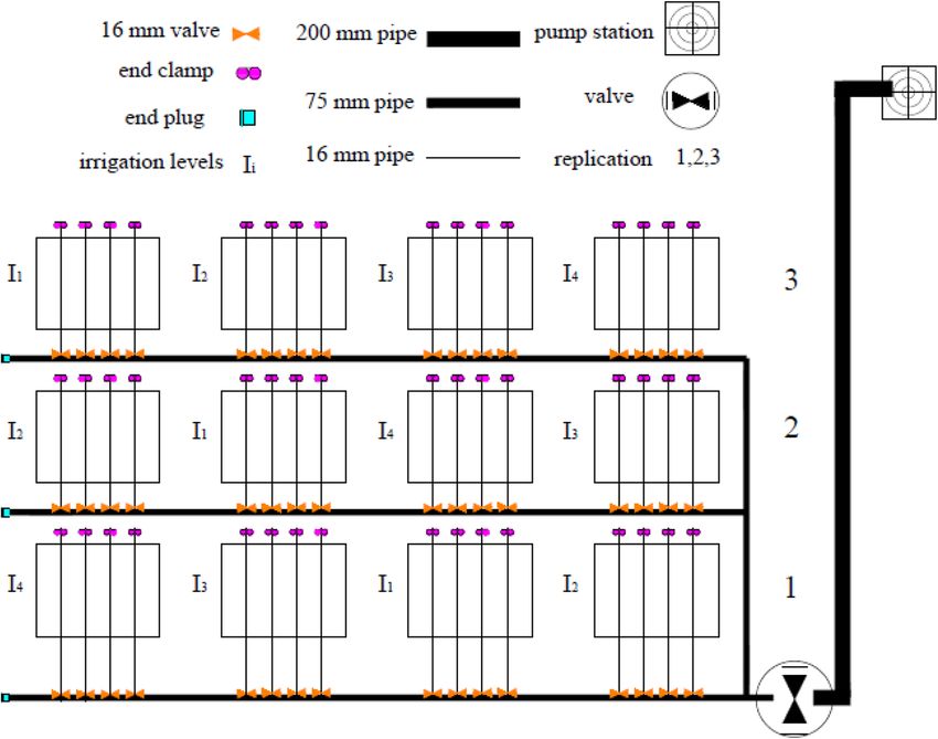
Figure 1. Plot layout of field experiment.
Experimental design and irrigation method. In the present study, the effect of different irrigation
water treatments on black grams was investigated. The experimental design was a randomized complete block
design with four aqueous treatments in three replications (Fig. 1). Water treatments included 50% ( I1), 75% ( I2),
100% (I3) or the control treatment, and 125% (I4) of crop water requirement. To determine the water require-
ment, meteorological parameters were obtained from the meteorological station of the Faculty of Agriculture
of Urmia University, and the reference evapotranspiration ( ETo) was calculated by V3.1 E To Calculator24. The
equation used in this software to calculate ETo is the FAO-modified Penman–Monteith equation25. Using the
following equation, the ETo calculated by multiplying the crop coefficient (Kc)26 was generalized to the potential
evapotranspiration (ETc) values of black gram (Table 3).
ETc = Kc × ETo (1)
Immediately after transferring the seedling, an irrigation step was carried out to plant the seedlings in the field.
The black gram is used as a second crop in the area while water stress was applied in mid-July (tenth irrigation)
for optimal plant establishment. The irrigation water amounts for each treatment, E Tc and E
To, during the crop
growth period are presented in Table 4. Plant irrigation was performed during the growing season using a 16 mm
dripper pipe located next to each row21. The 16 mm dripper pipe had constant pressure and the flow rate of emit-
ters was 4 L h-1. At the beginning of each 16 mm pipe, a 16 in 16 mm valve was used to control water stress over
time21. According to soil analysis, four fertilizer treatments were used to prevent nutrient deficiency27 and these
four treatments received equal amounts of fertilizers28. Fertilizer was used as a spray and soil fertilizers (Table 1).
Weather data. The meteorological parameters of the region including minimum, maximum and mean
temperature, minimum and maximum relative humidity, wind speed, precipitation and sunshine hours were
obtained during the present study from the Meteorology Station of Urmia University, which was the closest
meteorology station to the research area (Table 5). The WatchDog meteorological device installed around the
Scientific Reports | (2021) 11:869 | https://doi.org/10.1038/s41598-020-79516-3 4
Vol:.(1234567890)www.nature.com/scientificreports/
No Irrigation date Irrigation depth (mm) No Irrigation date Irrigation depth (mm)
1 11 June 15.62 12 26 July 22.24
2 14 June 11.28 13 30 July 28.60
3 18 June 17.20 14 2 August 21.14
4 21 June 14.84 15 6 August 27.74
5 25 June 18.53 16 9 August 21.27
6 28 June 15.12 17 13 August 28.11
7 2 July 24.57 18 16 August 25.67
8 5 July 18.51 19 20 August 24.57
9 12 July 47.98 20 27 August 47.67
10 19 July 48.36 21 3 September 49.34
11 23 July 30.49 – – –
Table 3. Black gram irrigation scheduling for control treatment (I3), during 2017 growing seasons.
Deficit irrigation Full irrigation Additional irrigation
I1 I2 I3 I4
Treatments (50%) (75%) (100%) (125%) ETc ETo
Total 279.41 419.12 558.82 698.53 502.94 554.70
Table 4. Irrigation amounts and ETo (mm), during 2017 growing seasons. ETo: reference evapotranspiration.
Month
Parameter May June July August September October
Air temp.mean (°C) 18.7 24 27.4 26.9 22.2 14.4
Air temp.max (°C) 24.9 31.3 34.5 34.2 29.4 21
Air temp.min (°C) 12.5 16.7 20.2 19.6 15.1 7.9
Relative humiditymax (%) 65 54 50 52 57 63
Relative humiditymin (%) 26 24 25 29 35 35
Wind speed (m s-1) 7 5 4 3 4 R
Precipitation (mm) 15.1 0 0 2.2 0 3.3
Hours of bright sunshine (h day−1) 309.8 341.9 344.4 349 296.5 255.4
Table 5. Average and sum monthly weather parameters, during 2017 growing seasons21.
farm was also used to obtain air temperature and relative humidity data over 10 min intervals to calculate air
vapor pressure deficit, and the data obtained from this device was inserted by a cable and the SpecWare 9 soft-
ware into the laptop21.
Plant measurements. Infrared thermometers (IRTs). In this study, the FLUKE Mini IR62 infrared device
was used to measure the canopy temperature ( Tc). One of the characteristics of all infrared devices is a special
feature called field of view. The field of view is the maximum angle between the rays coming from the object
being measured (the leaves of the black gram in the present study) received by the device. The larger the field of
view, the larger the image size measured by the device. Furthermore, the greater the distance of the device to the
target being measured the greater the field of view. Therefore, the field of view of the device is expressed as D:S
which is the ratio of the object diameter (point size or object diameter) to the distance from the device. The D:S
ratio of the infrared thermometer in the present study was 10:1.
Tc of black gram was not measured from planting to 10th July due to its small size and field of view of the
device12. Tc was measured from four geographical directions for each treatment (with three replications) when it
was sunny and cloudless6,28. Measurements were made on different leaves of black gram at an angle of 30° to 45°
to the horizon and an average Tc was obtained from an average 12 readings for each treatment28. Generally, for
each treatment in a single day, 84 T c readings were obtained in 7 h (8:50 to 14:50). To obtain the lower baseline
equation of the method of Idso et al.10 (Eq. (2)), Tc of black gram was measured for control treatment ( I3) from
8:50 to 14:50 in the post-irrigation d ays6. Meantime, in a bid to determine the experimental CWSI (Eq. (5)) and
the calculation of (Tc − Ta)m, Tc of black gram was measured from 11:50 to 14:50 in the pre-irrigation days for all
Scientific Reports | (2021) 11:869 | https://doi.org/10.1038/s41598-020-79516-3 5
Vol.:(0123456789)www.nature.com/scientificreports/
three treatments ( I1, I2 and I 3). CWSI values were calculated for the four growth stages of black gram including
floral induction-flowering, pod formation, seed and pod filling and physiological maturity.
Crop water stress index (CWSI). To investigate and describe the CWSI, a relationship based on two
parameters of (Tc − Ta) and AVPD is presented as follows10, and the line obtained by this equation is called the
lower baseline (L.L)6:
16.78Ta −116.9 RH
(Tc − Ta )L.L = a − b(AVPD) = a − b 10 × e Ta +237.3
× 1− (2)
100
where Tc is the canopy cover temperature (°C), Ta air temperature (°C), AVPD air vapor pressure deficit (mbar),
RH relative humidity (%), a and b are the different constant coefficients for crops and fruit trees. The lower
baseline is a special characteristic of each plant and represents the conditions where the plant has no limitations
on root water supply, and the air vaporization rate is at its maximum10. The upper baseline (U.L) also represents
the maximum (Tc − Ta) expected. The upper baseline status is obtained using the following relation10:
(Tc − Ta )U.L = a + b(AVPG) = a + b{es (Ta + a) − es (Ta )} (3)
17.27×Ta 1000
es (Ta ) = 0.6108 × e 237.3+Ta × (4)
101
where AVPG is the air vapor pressure gradient (mbar) and coefficients a and b are obtained from the lower
baseline (Eq. (2)). The empirical CWSI is also calculated by the following equation10:
(Tc − Ta )m − (Tc − Ta )L.L
CWSI = (5)
(Tc − Ta )U.L − (Tc − Ta )L.L
where (Tc − Ta)m is the difference between the canopy temperature and air temperature (pre-irrigation) at the
time of measurement (°C), (Tc − Ta)L.L is the difference between the canopy temperature and air temperature
(post-irrigation), which is obtained from the lower baseline equation. (Tc − Ta)U.L is a constant for the upper
baseline (post-irrigation).
Relative water content (RWC). Relative water content (RWC) of black gram leaves was measured four
times during crop growth period for each treatment (with three replications). RWC measurements were per-
formed during four days (before and after irrigation) every other week. On the days of measurement, two to
three adult and young leaves in the direction of the sunlight were cut from each plot after Tc measurement at
the maximum stress time. They were placed in plastic bags and transferred to the laboratory immediately21. The
RWC values were obtained by the following Eq. :29
FW − DW
RWC = (6)
TW − DW
where FW is fresh leaf weight (g), T W leaf weight at full turgidity (g) and D
W leaf weight when dried in oven
(g). The FW value was obtained after the leaves were removed from the crop. The leaves were then immersed in
distilled water for four hours. After achieving equilibrium, the leaves were removed by forceps and dried gently
and their weight ( T W) was measured. Finally, the leaves were placed in a paper bag to dry in the oven at 70 °C
btained29,30.
for 24 h, so that their dry weight (DW) is o
Leaf water potential (LWP). A relatively quick way to measure the water potential in large pieces of crop
tissues, such as leaves and stems, is to use a pressure chamber/bomb. This technique assumes that the water
pressure within vasculum is close to the average pressure potential of the entire organ because in most cases the
osmotic pressure of the vasculum is low. According to Stegman31, a pressure bomb measures the compressive
or expansive potential of the vasculum. However, because the osmotic potential of the vascular juice is usually
insignificant compared to the compressive potential, the negative pressure value in the pressure chamber is often
taken as the potential of the entire leaf. The pressure bomb is made of a hollow chamber to accomodiate the leaf
specimen. The leaf specimen is used through a gasket to hold the petiole. There is also a pressure capsule that
draws compressed air into the chamber. On the other hand, the same chamber is also connected to a barometer.
The leaf is placed into the chamber in a way that the petiole remains outside, and as the valve of the compressed
air capsule opens, the pressure inside the chamber gradually increases. The leaf wrinkles (wilts) and reaches a
pressure point where a drop comes out of the petiole. Just when the first drop comes out of the petiole, the pres-
sure is read on the machine.
The procedure was that in the afternoon, when the LWP reached its lowest (2–3 p.m. local time), the leaf
samples, which were completely exposed to sunlight, were selected from each treatment plot (three replications).
After each leaf sample was selected, it was cut by a sharp blade cutter and immediately put into the apparatus
and the pressure in the chamber was increased by opening the gas valve. As the pressure in the chamber was
increased by a handheld magnifying glass, the cut end of the leaf lamina remaining outside the device was care-
fully observed. This procedure was repeated for other samples and the mean LWP was obtained for three plots
in each treatment.
Scientific Reports | (2021) 11:869 | https://doi.org/10.1038/s41598-020-79516-3 6
Vol:.(1234567890)www.nature.com/scientificreports/
Soil measurements. Soil water (SW). The SW content is measured either directly (by weighting) or indi-
rectly (profile probe device or PR2). In direct methodology, the mass or volume of water is specifically measured,
but in indirect methodology, another factor that is related to the water content is measured first. Then the SW
content is estimated based thereupon. The PR2 device is manufactured in two models PR2/4 (with four sen-
sors) and PR2/6 (with six sensors) to measure the SW content in the vertical section. In PR2/6, six sensors are
installed on the 1 m bar that enters the soil, and it simultaneously measures the SW content at the depths of 10,
20, 30, 40, 60 and 100 cm. The sensor diameter of the machine is 25.4 mm and the special plastic pipes to be
installed in the soil have a diameter of 28 mm. SW content was measured three to four times per week (pre- and
post-irrigation)32 to the depth of root development at maximum stress times for all black gram treatments. In the
present study, a PR2/6 device calibrated with water weight data was used and tubes were installed in the middle
of each plot21.
Water retention curve. To measure the soil water retention curve (SWRC) in the laboratory, four intact
specimens were taken with two replicates from the soil at layers with the depths of 10–15 cm, and four from the
soil at layers with the depths of 30–35 cm by using sampling cylinders with the capacities of 100 cm3 and 50 cm3.
After saturation of the samples, 0, 20, 30, 100, 330, 1000, 3000, 8000 and 15,000 hPa matric suction were applied
to the samples using sand box and pressure plate devices. After equilibrium, their average weighted water con-
tent was measured33,34. The pressure plate consists of a chamber, such as a pressure-cooker, whosepressure could
be increased by a compressor. When the pressure reaches the desired potential point, it is relieved through the
drain valve and the lid is removed. Soil samples are removed quickly and their mass water content is measured.
The specimens are again inserted into the device and the lid is put on and the pressure is increased to the next
potential point. The mass moisture is again measured as above at this point.
The average soil porosity was calculated using the equation 1 − (BD/2.65) and is considered as saturated
moisture content. The SWRC model was fitted to the measured soil water retention data using RETC software.
The equation of van G enuchten35 is as follows:
1
θ(h) = θr + (θs −θr ) 1 + (αh)n n −1 (7)
where θ(h) denotes soil volumetric water content ( cm3 cm−3), h is the matric suction of the soil (hPa), θr is the
residual water content ( cm3 cm−3), θs represents saturated SW content ( cm3 cm−3), α is the inverse of suction at
the turning point (hPa-1) and n is the pore size distribution index (–)36.
Penetration resistance (Q) curve. The mechanical strength of the soil is the maximum resistance of soil
to mechanical stresses, without deformation and f racture37. The Q of soil can be measured by Automatic Micro
Penetrometer, which uses a proprietary software called KMP2 to allow the user to obtain accurate data on the Q
of the soil sample by adjusting the depth and velocity of the cone penetrating into the soil. The selectable diam-
eter of the cone is 1–5 mm. Six velocities varying from 2 to 30 mm min−1 were created for the penetration of the
cone Penetrometer into the soil sample. The display of Q values measured when the cone is inserted into the soil
allows the user to capture the data from the logger without storing them on the computer. An automatic record-
ing of Q values in text format or ASCI allows the user to read and use the input and output data (results) stored
in the Excel software. In the results section, every 0.5 mm penetration in the soil, one piece of data is recorded
and reported by the KMP2 software. This section also reports the total average Q, the highest and the lowest
measured values, and the measurement time.
To measure the soil Q characteristic curve (SPRC), five undisturbed soil samples from the 10–15 cm depth
layer and five undisturbed soil samples from the 30–35 cm depth received different water levels. To homogenize
the water distribution, the 10 soil samples were placed in plastic bags for four weeks. After water equilibrium
was obtained, the Q values were measured using an in vitro Automatic Micro Penetrometer with a penetration
rate of 5 mm min−1 in 3 replications with the vertices arranged in a triangle on 10 samples38. The water content
of soil samples was measured and converted to volumetric moisture content using BD values21. The SPRC model
was fitted to the measured soil Q data using the Solver program. In order to measure SPRC, van Genuchten’s35
adjusted model was applied in Eq. (8):
1
−1
(8)
n
Q = Ql + (Qh − Ql ) 1 + αQθ θ Qθ
nQθ
In this equation, Q is the soil penetration resistance (MPa), θ the soil volumetric moisture (cm3 cm−3), Ql the
lowest soil predicted resistance (MPa), Qh the highest soil predicted resistance (MPa), αQθ (cm3 cm−3), and nQθ(–)
the fitting parameters of the model related to the turning point and gradient of the function of mechanical resist-
ance to the SW content.
Model evaluation. To investigate the efficiency of regression models obtained in the results section of
the present study to estimate RWC, (Tc − Ta) and LWP, the correlation coefficient (R), root mean square error
(RMSE), mean absolute error (MAE) and mean relative error (MRE) were used39.
Scientific Reports | (2021) 11:869 | https://doi.org/10.1038/s41598-020-79516-3 7
Vol.:(0123456789)www.nature.com/scientificreports/
N
(Oi − Oi )(Pi − Pi )
i=1
R=
(9)
N N
(Oi − Oi )2 (Pi − Pi )2
i=1 i=1
1
N
RMSE =
(Oi − Pi )2 (10)
N
i=1
N
1
MAE = |Oi − Pi | (11)
N
i=1
N
1 |Oi − Pi |
MRE = (12)
N Oi
i=1
In these equations, N is the number of measurements (samples), i index of each model, Oi and P i measured
and predicted values, and Oi and Pi mean measured and predicted values. However, the results from the above
four criteria sometimes vary in different m odels40. The Ideal Point Error (IPE) index was used to select the best
model with the highest accuracy. This index combines the effects of four error criteria and helps choosing the
right model. The IPE index is based on identifying the ideal point in the n-dimensional space (n is the number
of statistical criteria to evaluate the models), which every models seeks to approach. The ideal point coordinates
should be RMSE = 0.0; MAE = 0.0; MRE = 0.0; R = 1.0. The IPE index (Eq. (13)) indicates how far the model is
from the ideal p oint39.
2
2
2
2 21
RMSEi − 0.0 MAEi − 0.0 MREi − 0.0 Ri − 1.0
IPEA = 0.25 + + + (13)
max(RMSE) max(MAE) max |MRE| 1/ max(R)
where, for the model i, max(x) is the maximum value of the x statistic between a groups of study models and
is used as a model performance standardization factor for each individual evaluation index. The value of the
IPE index varies from zero (best model) to one (worst model), and the closer to zero, the more appropriate the
model will b e39.
A careful examination of the original IPEA equation shows that there is a contradiction in the standardiza-
tion method applied to each component. In Eq. (13), the first three indices are standardized according to the
worst model performance, while the last index (R) is standardized according to the best model performance.
It should also be noted that standardization of R in the original IPEA equation is not designed for negative
values41. Equation (14) or I PEB represents an improved variant of the original equation, which includes a more
generalized and robust standardization procedure for R that can accommodate the full range [− 1, + 1]. I PEB is
also consistent with the method of standardization with regard to the worst-case model performance. So, the
new index eliminates the inconsistency (contradiction) of standardization of the original IPEA equation. This
correction can lead to a significant difference between the output of the original IPEA and the IPEB, especially
for the states containing medium or low R values41.
2
2
2
2 21
RMSEi MAEi MREi Ri − 1
IPEB = 0.25 + + + (14)
max(RMSE) max(MAE) max |MRE| min(R) − 1
Results and discussion
Baseline equations and CWSI. To calculate the lower baseline of the experimental method of Idso et al.10,
c of black gram was measured from 8:50 am to 02:50 pm. Lower baseline equations using this experimental
T
method for the four growth stages of black gram (floral induction-flowering, pod formation, seed and pod filling
and physiological maturity) are presented for different days after irrigation in Table 6. The correlation between
(Tc − Ta) and AVPD is also shown in Fig. 2. According to this figure, the range of AVPD and (Tc − Ta) for the four-
stage growth of black gram are, respectively, 4 to 46 mbar and 3 to − 7 °C. The lower baseline equations fitted to
the four growth stages can be used in different locations for black gram as long as the AVPD range has a wide
range42. As AVPD increases, (Tc − Ta) increases (in absolute value) while the rate of increase (Tc − Ta) decreases
with time6. Examination of the lower baseline relationships showed that the coefficients a and b were different
for each growth stage of the black gram. There was also a negative gradient for all four growth stages of crop
(Table 6). Due to the differences in the values of these coefficients, one can point to the difference of water uptake
potential and also the rate of transpiration during plant growth stages21.
The upper baseline values were calculated using the Idso et al.10 method for the four growth stages of black
gram as 2.63, 6.25, 2.79 and 7.73 °C, respectively (Table 6). According to CWSI-based irrigation scheduling
research, it is clear that the upper baseline depends on the crop species, crop variety and climatic conditions
of each area6,21. The specificity of the lower and upper baselines for each crop indicates that at maximum
Scientific Reports | (2021) 11:869 | https://doi.org/10.1038/s41598-020-79516-3 8
Vol:.(1234567890)www.nature.com/scientificreports/
Date Growth stages Lower baseline Upper baseline R2 p-value
July 11 to July 21 Flowral induction-Flowering (Ta − Tc)L.L = 1.8391 − 0.1836(AVPD) (Ta − Tc )U.L = 2.63 0.88 < 0.001
(Ta − Tc )L.L = 4.2821 −
July 25 to August 4 Pod formation (Ta − Tc )U.L = 6.25 0.57 < 0.010
0.1723(AVPD)
(Ta − Tc )L.L = 2.3767 −0.0742
August 8 to August 22 Seed and Pod filling (Ta − Tc )U.L = 2.79 0.70 < 0.001
(AVPD)
( Ta − Tc )L.L = 5.4043 − 0.172
August 26 to September 5 Physiological maturity (Ta − Tc )U.L = 7.73 0.85 < 0.001
(AVPD)
Table 6. Equations for lower and upper baselines by Idso et al.32 for four stages of black gram growth. dTL.L:
lower baseline; dTU.L: upper baseline; AVPD: air vapor pressure deficit; R2: coefficient of determination.
Figure 2. Lower and upper baselines for four stages of black gram growth.
transpiration, each crop reacts to a variety of stresses (water, salinity, fertility, etc.) and meteorological param-
eters (temperature, wind speed, relative humidity, etc.); and the transpiration value differs in various c rops21.
The lower and upper baseline equations at the different dates of the black gram growth period are presented
in Table 7. According to this table, the values of a and b coefficients were different at different days of the crop
growth for the lower baseline equations, the reasons for which were discussed in the previous section. The R2
of the lower baseline equations ranges from 0.82 to 0.98, and the high value of R2 and the low P-value represent
acceptable accuracy of the regression equations. It should be noted that the range of the upper baseline equations
was from 2.46 to 9.90 °C, which indicates a complete stress condition during the crop growth period.
After formulating the lower and upper baseline equations by Idso’s et al.10 method for the four growth stages
of black gram (Table 6) and also calculating the mean ( Tc − Ta) on the pre-irrigation days (11:50 am to 02:50 pm),
CWSI values were calculated for treatments I 1, I2 and I 3 (Table 8). According to Table 8, the CWSI threshold values
for the control treatment (I3) in the four growth stages were 0.14, 0.08, 0.22, and 0.15, respectively.Moreover, the
mean CWSI values during the growth period of the black gram for the three treatments of 50, 75 and 100% of
crop water requirement were calculated to be 0.37, 0.23 and 0.15, respectively. The maximum CWSI for all three
treatments occurred on August 8 to August 22 (pod and seed filling stage) and the highest CWSI was related to
severe irrigation deficit ( I1) treatment.
Scientific Reports | (2021) 11:869 | https://doi.org/10.1038/s41598-020-79516-3 9
Vol.:(0123456789)www.nature.com/scientificreports/
Date Lower baseline R2 Upper baseline
July 13 (Ta − Tc)L.L = 4.4634 − 0.3115 (AVPD) 0.98 (Ta − Tc)U.L = 7.44
July 20 (Ta − Tc)L.L = − 3.811 − 0.2297 (AVPD) 0.97 ( Ta − Tc)U.L= 6.26
July 27 ( Ta − Tc)L.L = 3.5435 − 0.1771 (AVPD) 0.94 ( Ta − Tc)U.L= 5.22
August 3 ( Ta − Tc)L.L = − 4.4407 − 0.1489 (AVPD) 0.91 ( Ta − Tc)U.L = 6.19
August 10 (Ta − Tc)L.L = − 4.6014 − 0.1391 (AVPD) 0.93 ( Ta − Tc)U.L = 6.31
August 17 (Ta − Tc)L.L = 2.1254 − 0.080(AVPD) 0.82 ( Ta − Tc)U.L = 2.46
August 21 ( Ta − Tc) L.L= − 4.9039 − 0.1347(AVPD) 0.96 (Ta − Tc)U.L = 6.72
August 28 ( Ta − Tc)L.L = − 6.4275 − 0.2149(AVPD) 0.97 (Ta − Tc)U.L = 9.90
September 4 ( Ta − Tc)L.L = − 4.3143− 0.1268(AVPD) 0.83 (Ta − Tc)U.L = 5.67
Table 7. Equations for lower and upper baselines at different dates of the black gram growth period.
(Tc—Ta)L.L: lower baseline; (Tc—Ta)U.L: upper baseline; AVPD: air vapor pressure deficit; R2: coefficient of
determination.
Growth stages I1 (50%) I2 (75%) I3 (100%)
Flowral induction-flowering – – 0.14
Pod formation 0.28 0.13 0.08
Seed and Pod filling 0.47 0.28 0.22
Physiological maturity 0.35 0.27 0.15
Average 0.37 0.23 0.15
Table 8. CWSI threshold and average values during black gram growth period.
Date Growth stages Scheduling relationships
July 11 to July 21 Flowral induction-flowering (Ta − Tc)c = 1.9498 − 0.1579 (AVPD)
July 25 to August 4 Pod formation (Ta − Tc)c = 4.4395 c − 0.1585(AVPD)
August 8 to August 22 Seed and Pod filling (Ta − Tc)c = 2.4676 c − 0.0578 (AVPD)
August 26 to September 5 Physiological maturity (Ta − Tc)c = 5.7532 c − 0.1462(AVPD)
Table 9. Relationships used for black gram irrigation scheduling. (Tc—Ta)c: the permitted difference between
the canopy temperature and air temperature; AVPD: air vapor pressure deficit.
The CWSI empirical m ethod10 has been used in various research for plant irrigation management. In the study
of CWSI threshold for the soybean, the value of 0.18 was obtained43. Also, in other investigations on chili pepper
and eggplant under surface drip irrigation, CWSI threshold values were 0.20 and 0.26, r espectively28,44. It should
be noted that so far no research has been done to evaluate water stress index of black gram to be compared with
the results of the present study. The higher the SW content, the lower the ambient temperature will be. Thus, the
study treatments change the environmental conditions. Meantime, the crops that grow under stress will have
different physiological and morphological characteristics. Finally, by increasing water stress, the stomata of the
plant are closed and Tc, and thus CWSI would increase21,45.
Irrigation scheduling using of CWSI. In this study, CWSI was used for irrigation scheduling of black
gram (four growth stages). Since the lowest CWSI (0.15) for black gram was observed in the unstressed treat-
ment, this treatment was taken as the basis of irrigation scheduling if the black gram based on the experimental
method. The CWSI values obtained using Eq. (5) for the four growth stages of crop are presented in Table 8.
Therefore, using the CWSI values and Eq. (15), the equations required for irrigation scheduling of black gram
are presented in Table 9 for the four growth stages of the crop in Urmia.
(Tc − Ta )c − dTL.L
CWSIi = (15)
dTU.L − dTL.L
The parameters of Eq. (15) have already been described.
To determine the irrigation schedule, the values of Ta and RH must first be measured at 11:50 am to 02:50 pm
and then the AVPD is calculated. Finally, substituting AVPD in the existing equations Table 9, the allowed
(Tc − Ta)c value could be c alculated21. To determine the irrigation time, we can compare the ( Tc − Ta)m (mean
values calculated in the field) and (Tc − Ta)c (permissible values), in which case, three conditions occur: 1. If
the mean value of (Tc − Ta)m is less than (Tc − Ta)c, it’s too soon to irrigate the crop, 2. If greater than (Tc − Ta)m id
Scientific Reports | (2021) 11:869 | https://doi.org/10.1038/s41598-020-79516-3 10
Vol:.(1234567890)www.nature.com/scientificreports/
(a)
θr θs α n
Soil layer (cm) cm3 cm−3 hPa-1 (–) R2
10–15 0.000 0.488 0.123 1.084 0.982
30–35 0.000 0.450 0.035 1.083 0.972
(b)
Ql Qh αQθ n
Soil layer (cm) MPa cm−3 cm3 (–) R2
10–15 0.897 10.810 4.465 7.826 0.999
30–35 0.047 9.907 4.284 5.972 0.998
Table 10. Parameters of van Genuchten35 model for the SWRC (a) and modified van Genuchten35 model
for the SPRC (b) fitted to the measured data. θr and θs: residual moisture and soil saturation, respectively; α:
inverse suction in the turning point (air entry point); n: pore size distribution index; Ql and Qh: lowest (wet)
and maximum (dry) predicted soil penetration resistance, respectively; αQθ and nQθ: fitness parameters of
the model related to the turning point and slope of the mechanical strength function against soil water; R2 is
coefficient of determination.
R RMSE MAE MRE IPEA IPEB
Model Variables (%) (–) (–) (–) N p-value (–) (–)
1 (Tc − Ta) 44.1 0.027 0.022 0.028 64 0.000 0.806 0.865
2 SW 25 0.029 0.023 0.029 64 0.045 0.866 0.964
3 Q 23.1 0.029 0.023 0.029 64 0.064 0.873 0.975
4 RH 18.7 0.029 0.023 0.03 64 0.141 0.888 1.000
5 (Tc − Ta), SW 48.1 0.026 0.021 0.027 64 0.000 0.795 0.847
6 (Tc − Ta), Q 47.4 0.026 0.021 0.027 64 0.000 0.797 0.85
7 (Tc − Ta), RH 44.6 0.027 0.021 0.027 64 0.001 0.799 0.858
8 SW, Q 25.5 0.029 0.023 0.029 64 0.124 0.865 0.961
9 SW, RH 30.7 0.029 0.022 0.029 64 0.048 0.846 0.932
10 Q, RH 29.8 0.029 0.022 0.028 64 0.058 0.845 0.934
11 (Tc − Ta), SW, Q 48.4 0.026 0.021 0.027 64 0.001 0.795 0.846
12 (Tc − Ta), SW, RH 48.6 0.026 0.021 0.027 64 0.001 0.788 0.839
13 (Tc − Ta), Q, RH 48 0.026 0.021 0.027 64 0.001 0.789 0.786
14 (Tc − Ta), SW, Q, RH 48.8 0.026 0.021 0.027 64 0.003 0.787 0.783
15 SW, Q, RH 30.8 0.028 0.022 0.029 64 0.108 0.847 0.875
Table 11. Linear different models and statistical parameters for RWC estimating. R is correlation coefficient;
RMSE: root mean square error; MAE: mean absolute error; MRE: mean relative error; IPE: Ideal Point Error;
N is the number of measurements.
larger than ( Tc − Ta)c, the irrigation has been missed and in the third case, if ( Tc − Ta)c and ( Tc − Ta)m are equal, it
is to time for irrigation46.
Relations between plant and soil indices. Linear regression relationships–univariate. The use of clas-
sical methods to estimate and monitor the water depletion in the crop-soil system requires measurement of SW
content, crop properties or climatic variables. Unless a large number of samples are produced and interpreted,
these methods are time-consuming and provide a poor description of the overall situation of the field due to pro-
ducing point data47. Van Genuchten’s35 model fitting parameters in layers of 10 − 15 cm (surface) and 30 − 35 cm
(lower) depth are presented in Table 10 for the soil water retention curve (SWRC) of the black gram. According
to Table 10, van Genuchten’s35 model fitted well to the in vitro data because high values of R2 were obtained in
the surface and lower layers (Fig. 3a).
In this study, the I4 treatment was considered for soil ventilation porosity21 and sometimes, just because
the measurements (canopy temperature) have been made post-irrigation does not mean there are unstressed
conditions and in this case, the data of the treatment that received the highest amount of water can be used for
the rest of the treatments. The critical level of ventilation porosity is about 10% the ventilation porosity of root
growth48, and if the soil Q values are between 1.5 and 4 MPa, it restricts root development and 2 MPa (critical Q)
is the most acceptable v alue48. The soil Q content increased drastically by decreasing the soil moisture, thereby
causing the plant to be simultaneously affected by two types of stress, i.e. soil water deficit and soil Q increase49.
Scientific Reports | (2021) 11:869 | https://doi.org/10.1038/s41598-020-79516-3 11
Vol.:(0123456789)www.nature.com/scientificreports/
R RMSE MAE MRE IPEA IPEB
Model Variables (%) (°C) (°C) (–) N p-value (–) (–)
1 SW 50.5 2.47 1.97 − 0.43 140 0.000 0.740 0.771
2 Q 43.8 2.57 2.03 − 0.44 140 0.000 0.769 0.807
3 RH 12.1 2.84 2.30 − 0.29 140 0.154 0.817 0.902
4 AVPD 11.9 2.84 2.31 − 0.40 140 0.16 0.853 0.935
5 SW, Q 50.9 2.46 1.98 − 0.41 140 0.000 0.734 0.765
6 SW, RH 50.6 2.46 1.97 − 0.40 140 0.000 0.730 0.761
7 SW, AVPD 55.4 2.38 1.87 − 0.56 140 0.000 0.785 0.809
8 SW, Q, RH 51.0 2.46 1.98 − 0.40 140 0.000 0.728 0.759
9 SW, Q, AVPD 56.0 2.37 1.87 − 0.53 140 0.000 0.768 0.791
10 Q, RH 44.6 2.56 2.02 − 0.39 140 0.000 0.745 0.783
11 Q, AVPD 47.7 2.51 1.99 − 0.55 140 0.000 0.809 0.840
12 RH, AVPD 47.7 2.51 1.99 − 0.27 140 0.000 0.688 0.724
13 SW, Q, RH, AVPD 72.9 1.96 1.55 − 0.30 140 0.000 0.559 0.571
14 SW, RH, AVPD 72.9 1.96 1.55 − 0.30 140 0.000 0.558 0.571
15 Q, RH, AVPD 69.8 2.05 1.62 − 0.31 140 0.000 0.582 0.597
Table 12. Linear different models and statistical parameters for (Tc − Ta) estimating. R is correlation coefficient;
RMSE: root mean square error; MAE: mean absolute error; MRE: mean relative error; IPE: Ideal Point Error;
N is the number of measurements.
Model Variables R (%) RMSE (bar) MAE (bar) MRE (–) N p-value IPEA (–) IPEB (–)
1 (Tc − Ta) 7.9 2.84 2.24 − 0.270 28 0.689 0.884 0.982
2 SW 15.1 2.82 2.22 − 0.271 28 0.442 0.877 0.961
3 Q 9.7 2.84 2.21 − 0.270 28 0.624 0.880 0.975
4 RWC 35.3 2.67 2.11 − 0.247 28 0.065 0.816 0.869
5 RH 1.9 2.85 2.22 − 0.270 28 0.926 0.885 0.995
6 (Tc − Ta), SW 15.9 2.81 2.22 − 0.270 28 0.728 0.875 0.958
7 (Tc − Ta), Q 11.3 2.83 2.22 − 0.270 28 0.850 0.880 0.972
8 (Tc − Ta), RWC 35.8 2.66 2.14 − 0.249 28 0.180 0.821 0.874
9 (Tc − Ta), RH 8.3 2.84 2.24 − 0.271 28 0.918 0.886 0.983
10 SW, Q 29.2 2.72 2.12 − 0.252 28 0.328 0.831 0.893
11 SW, RWC 35.9 2.66 2.11 − 0.249 28 0.179 0.817 0.870
12 SW, RH 16 2.81 2.20 − 0.267 28 0.723 0.870 0.953
13 Q, RWC 35.4 2.66 2.11 − 0.248 28 0.188 0.817 0.871
14 Q, RH 10.2 2.83 2.20 − 0.268 28 0.878 0.876 0.970
15 RWC, RH 36.2 2.66 2.11 − 0.250 28 0.174 0.818 0.870
16 (Tc − Ta), SW, Q 29.8 2.72 2.11 − 0.251 28 0.517 0.828 0.890
17 (Tc − Ta), SW, RWC 36.2 2.66 2.14 − 0.251 28 0.330 0.822 0.874
18 (Tc − Ta), SW, RH 16.5 2.81 2.21 − 0.268 28 0.880 0.872 0.955
19 (Tc − Ta), SW, Q, RWC, RH 41.8 2.59 2.09 − 0.243 28 0.478 0.800 0.844
20 (Tc − Ta), SW, Q, RWC 40.5 2.60 2.12 − 0.243 28 0.368 0.805 0.851
21 (Tc − Ta), SW, Q, RH 29.9 2.72 2.12 − 0.252 28 0.691 0.829 0.890
22 SW, Q, RWC, RH 41.1 2.6 2.06 − 0.241 28 0.349 0.795 0.841
23 SW, Q, RWC 40.1 2.61 2.09 − 0.242 28 0.232 0.801 0.848
24 SW, Q, RH 29.2 2.72 2.12 − 0.253 28 0.535 0.831 0.894
25 Q, RWC, RH 36.2 2.66 2.10 − 0.249 28 0.329 0.816 0.868
Table 13. Linear different models and statistical parameters for LWP estimating. R is correlation coefficient;
RMSE: root mean square error; MAE: mean absolute error; MRE: mean relative error; IPE: Ideal Point Error;
N is the number of measurements.
Scientific Reports | (2021) 11:869 | https://doi.org/10.1038/s41598-020-79516-3 12
Vol:.(1234567890)www.nature.com/scientificreports/
Figure 3. van Genuchten35 function fitted to the SWRC (a) and modified van Genuchten35 model fitted to the
SPRC (b) data; well-known critical Q = 2.0 MPa is shown on the graph.
Figure 4. Linear relations between RWC and Q (a) and RWC and SW (b) indices.
The fitting parameters of van Genuchten’s35 model in the surface and lower layers (Fig. 3b) for the soil Q curve
(SPRC) are also presented in Table 10 and high values for R2 are obtained due to a better control of conditions
and uniform water distribution in the samples taken from the two layers38. In Fig. 3b, the well-known critical
Q has been identified, and the critical Q value of 2 MPa was observed for the black gram in the lower layer at
about 0.315 cm3 cm−3 and at the surface layer at about 0.305 cm3 cm−3; so, the water contents of these two layers
were close together. In the SWRC of the black gram (Fig. 3a) there was no significant difference in the pore size
distribution, so the SWRC (Fig. 3a) and SPRC (Fig. 3b) curves were overlapped and are similar to one another.
Water and temperature stresses are among the most important abiotic stresses that occur at different growth
stages in arid and semiarid areas50. Unfortunately, in recent years crop production (such as rice, maize and wheat)
has declined sharply in many parts of Asia due to rising water stress, so breeders are more likely to cope with
this problem through selecting drought resistant cultivars with high water use efficiency. They use agronomic,
physiological and biological methods for this purpose51. Regression equations were extracted for plant and
soil indices measured simultaneously at maximum stress hours during the growth period of black gram (one
of drought tolerant crops). The relationship between RWC and soil indices (Q and SW), relationship between
(Tc − Ta) and soil and plant indices (Q, SW and RWC), the relationship between leaf water potential (LWP) and
soil and plant indices (Q, SW and RWC) as well as with the plant indices and meteorological parameters (Tc − Ta)
are observed (Figs. 4, 5 and 7).
According to the Hofler d iagram30 and the critical limit of RWC (0.80), if the value of 0.80 is assumed as the
critical limit of RWC in the black gram, according to Fig. 4a,b, the critical value of Q and SW is − 0.3 MPa and 0.34
cm3 cm−3 (matric potential = 520 hPa). The critical values of Q (with negative coefficient) and SW obtained for
black gram are not reasonable values since Q cannot be less than zero. Therefore, it is not acceptable. Moreover,
the accuracy of regression equations obtained for black gram is low. It should be noted that the Hofler diagram
has been obtained for specific crops such as maize and wheat, while the black gram is a drought tolerant crop.
According to Fig. 4a,b, an increase in the soil Q (with decreasing SW) decreased the RWC value of the leaf only
slightly (with low gradient). The permissible ( Tc − Ta)c value was also calculated for the entire growth period of
black gram and was about − 0.036 °C, which can be taken as the critical value ( Tc − Ta). Consequently, the criti-
cal values of Q, SW and RWC for the entire growth period are 10.43 MPa, 0.14 c m3 cm−3 and 0.76, respectively.
Scientific Reports | (2021) 11:869 | https://doi.org/10.1038/s41598-020-79516-3 13
Vol.:(0123456789)www.nature.com/scientificreports/
Figure 5. Linear relations between (Tc − Ta) and Q (a), (Tc − Ta) and SW (b), and (Tc − Ta) and RWC (c) indices.
It should be noted that the values of SW and Q were lower and higher than expected, respectively, although
black gram is a drought tolerant plant. So, it is advisable to repeat these values for other conditions. According
to Fig. 5a,b, changes in (Tc − Ta) relative to Q and SW are almost linear, that is, as the SW decreases (increasing
Q), the value of (Tc − Ta) increases. According to Fig. 5c, by decreasing RWC, (Tc − Ta) increases and therefore, it
would increase by decreasing AVPD.
According to Khorsand et al.21 study on maize, with loss of soil water, the RWC of the crop lowers (higher
gradient), but some crops such as black gram that are more tolerant lower their RWC less by reducing their tran-
spiration or managing their water more effrectively. In other words, their RWC decreases with a lower gradient
(Fig. 4b), indicating that the leaf water content is lost less rapidly. RWC is one of the important physiological
indices that has good correlation with resistance to drought stress. By increasing the drought stress, the RWC of
the leaf decreases52. Cultivars that are able to maintain a greater leaf RWC under reduced SW content will have
greater resistance to water loss. In other words, they have a higher ability to absorb and retain water. In a study
by Siddique et al.53, increased drought stress reduced the RWC value of wheat, and typically, drought tolerant
cultivars show higher RWC than cultivars susceptible to drought stress.
According to the field data obtained from black gram cultivation in West Azerbaijan Province, this crop is
highly resilient tolerance to water deficit stress and the ratio of root to the shoot in higher in this crop. Typically,
species with higher R/S ratios are more susceptible to drought stress. Singh et al.54 stated that crops with longer
roots, a higher number of lateral roots, root length and higher R/S are more resistant to water deficit and drought
stress. The root of black gram (leguminosae), which is a dicot, is right-sided, with two important characteristics:
(1) Absorbing water from higher depth, and (2) water-nutrition retaining root. A decrease in leaf RWC can be
due to a decrease in the amount of water absorbed from the soil by the roots or due to evaporation from the
stomata55. Moreover, the high RWC in water deficit conditions can be related to the behavior of the stomata and
root system of the c rop56, because retaining the water content of the crop requires deep roots to absorb w ater57.
Drought-tolerant plants use several features to reduce transpiration:
1. Morphological features including: (a) Number of stomata; (b) Size of stomata; (c) Location of stomata; (d)
The fluffs existing on the leaf surface; (e) Leaf turndown (epinasty or downward bending in leaves)58: We
observed this phenomenon (epinasty) in the black gram at the peak of the maximum stress hour (03:00 pm),
and this may be another reason for the decrease in transpiration and non-variation of RWC; (f) Leaf angle;
(g) Wax layer on leaf surface.
2. Physiological features including: (a) Closure of stomata: With higher production of Abscisic Acid (ABA),
the wild species can close their stomata more quickly and drastically (transpiration decreases, i.e. the RWC
does not change significantly). A sharp decrease in the stomatal conductance with slight variations of RWC
Scientific Reports | (2021) 11:869 | https://doi.org/10.1038/s41598-020-79516-3 14
Vol:.(1234567890)You can also read