Event and seasonal hydrologic connectivity patterns in an agricultural headwater catchment - HESS
←
→
Page content transcription
If your browser does not render page correctly, please read the page content below
Hydrol. Earth Syst. Sci., 25, 2327–2352, 2021
https://doi.org/10.5194/hess-25-2327-2021
© Author(s) 2021. This work is distributed under
the Creative Commons Attribution 4.0 License.

Event and seasonal hydrologic connectivity patterns
in an agricultural headwater catchment
Lovrenc Pavlin1,2 , Borbála Széles1,2 , Peter Strauss3 , Alfred Paul Blaschke1,4 , and Günter Blöschl1,2
1 Centre for Water Resource Systems, Vienna University of Technology, Vienna, Austria
2 Instituteof Hydraulic Engineering and Water Resources Management, Vienna University of Technology, Vienna, Austria
3 Federal Agency of Water Management, Institute for Land and Water Management Research, Petzenkirchen, Austria
4 Interuniversity Cooperation Centre Water & Health, Vienna, Austria

Correspondence: Lovrenc Pavlin (pavlin@hydro.tuwien.ac.at)

Received: 15 July 2020 – Discussion started: 30 July 2020
Revised: 24 February 2021 – Accepted: 21 March 2021 – Published: 29 April 2021

Abstract. Connectivity of the hillslope and the stream is          1   Introduction
a non-stationary and non-linear phenomenon dependent on
many controls. The objective of this study is to identify these
controls by examining the spatial and temporal patterns of         Hydrologic connectivity is an important control on runoff
the similarity between shallow groundwater and soil mois-          generation in response to precipitation events (van Meerveld
ture dynamics and streamflow dynamics in the Hydrologi-            et al., 2015; Penna et al., 2015; Zuecco et al., 2016). It is
cal Open Air Laboratory (HOAL), a small (66 ha) agricul-           usually defined as the ability of water, solutes or microor-
tural headwater catchment in Lower Austria. We investigate         ganisms to move from one landscape unit to another along
the responses to 53 precipitation events and the seasonal dy-      a water flowpath (Blume and van Meerveld, 2015; Saffar-
namics of streamflow, groundwater and soil moisture over 2         pour et al., 2016; Vidon and Hill, 2004). In the headwa-
years. The similarity, in terms of Spearman correlation coef-      ter catchments, the connection between the hillslope and the
ficient, hysteresis index and peak-to-peak time, of groundwa-      stream is established either when the groundwater table rises
ter to streamflow shows a clear spatial organization, which is     above the confining layer at the upland–riparian zone inter-
best correlated with topographic position index, topographic       face to a more permeable layer or when a permeable layer
wetness index and depth to the groundwater table. The sim-         gets continuously saturated (Ocampo et al., 2006; Tromp-
ilarity is greatest in the riparian zone and diminishes further    van Meerveld and McDonnell, 2006; Vidon and Hill, 2004).
away from the stream where the groundwater table is deeper.        Changes in connectivity could be related to the differences
Soil moisture dynamics show high similarity to streamflow          in hydrologic behaviour patterns by considering the underly-
but no clear spatial pattern. This is reflected in a low corre-    ing controlling processes (Western et al., 2001). Therefore,
lation of the similarity with site characteristics. However, the   the analysis of groundwater dynamics in different landscape
similarity increases with increasing catchment wetness and         units and across temporal scales is an important step toward
rainfall duration. Groundwater connectivity to the stream on       understanding when and where the connectivity occurs.
the seasonal scale is higher than that on the event scale, in-        Groundwater (GW) and soil moisture (SM) dynamics ex-
dicating that groundwater contributes more to the baseflow         hibit spatial patterns that can depend on site characteristics
than to event runoff.                                              such as soil depth (Penna et al., 2015; Rosenbaum et al.,
                                                                   2012), soil type (Gannon et al., 2014), land cover (Bach-
                                                                   mair et al., 2012; Emanuel et al., 2014) and topography
                                                                   (Bachmair and Weiler, 2012; Rosenbaum et al., 2012). Sur-
                                                                   face and subsurface topography were shown to be important
                                                                   controls on the spatial distribution of groundwater dynam-
                                                                   ics and connectivity of the hillslope to the riparian zone and

Published by Copernicus Publications on behalf of the European Geosciences Union.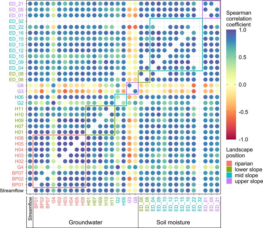
2328       L. Pavlin et al.: Event and seasonal hydrologic connectivity patterns in an agricultural headwater catchment

the stream (Bachmair and Weiler, 2012; Detty and McGuire,          controls on the flowpath activation and conversely connec-
2010; Loritz et al., 2019; Tromp-van Meerveld and McDon-           tivity of different landscape units.
nell, 2006). Local slope affects the rainfall drainage. The ups-      Despite significant improvement in our understanding of
lope contributing area affects the amount of water that could      the hillslope connectivity to the stream, the site and event
be supplied to a given location as quantified by the Topo-         characteristic controls on the groundwater and soil moisture
graphic Wetness Index (TWI) (Beven and Kirkby, 1979). The          dynamics in relation to the streamflow on the event and sea-
TWI was shown to be a good predictor of hydrologic connec-         sonal scales are not fully understood. Furthermore, in agri-
tivity in steep forested and grassland catchments with shal-       cultural catchments, the hydrologic connectivity is also im-
low groundwater table (Emanuel et al., 2014; Loritz et al.,        portant for its impact on the solute load (e.g. nitrate and
2019; Rinderer et al., 2016, 2017) and abandoned terraces          dissolved organic carbon) in streams (Aubert et al., 2013;
(Lana-Renault et al., 2014; Latron and Gallart, 2008). How-        Zhang et al., 2011). Understanding of catchment connec-
ever, in some studies, this was true only during specific wet-     tivity could, therefore, lead to better agricultural practices.
ness conditions, for certain types of rainstorms (Bachmair         However, except for Saffarpour et al. (2016) and Ocampo et
and Weiler, 2012) or when terrain freezes over (Coles and          al. (2006), the recent connectivity studies’ focus was less on
McDonnell, 2018).                                                  the agricultural catchments compared to forested and alpine
   Antecedent wetness conditions and precipitation event           catchments. Here we present an investigation of connectivity
characteristics, such as rainfall intensity and depth, have also   between the groundwater, soil moisture and streamflow in
been identified as controls on groundwater and soil mois-          terms of the similarity of their dynamics and how it is related
ture responses to rainfall events (Dhakal and Sullivan, 2014;      to the site and event characteristics. We analyse the similarity
Penna et al., 2015; Rosenbaum et al., 2012; Saffarpour et al.,     between groundwater and soil moisture monitoring stations
2016). Penna et al. (2015) and Detty and McGuire (2010)            and the streamflow at the catchment outlet for 53 events and
found that wetter antecedent conditions and higher rainfall        over 2 years. We address the following questions.
depth increased groundwater peaks, the number of activated
                                                                       1. What are the spatial and temporal patterns in the rela-
wells and the spatial extent of the subsurface flow network
                                                                          tionship between the streamflow, groundwater and soil
in a steep catchment in the Italian Alps and a forested catch-
                                                                          moisture responses to precipitation events in an agricul-
ment in New Hampshire, respectively. In contrast, groundwa-
                                                                          tural headwater catchment?
ter in the Black Forest in Germany responded more weakly
and slowly during wet conditions than during dry conditions            2. Is the relationship between the streamflow and ground-
when preferential flowpaths were activated (Bachmair et al.,              water or soil moisture dynamics more related to site or
2012). Rosenbaum et al. (2012) found that the rainfall char-              event characteristics?
acteristics, especially rainfall intensity, were the dominant
controls on the soil moisture responses during the wetting             3. How are event and seasonal connectivities of ground-
period in the hilly forested test site Wüstenbach, Germany.               water and soil moisture to streamflow related?
   Different processes may govern seasonal and event dy-
namics of streamflow, groundwater and soil moisture in the         2     Methods
catchment. Slower processes or flowpaths with lower celer-
ity are usually more relevant on the seasonal scale, while the     2.1    Study site
quicker processes control the event responses and do not af-
fect the seasonal dynamics. Event dynamics is superimposed         The research area of this study is the HOAL (Hydrologi-
on the seasonal dynamics, which provide the initial condi-         cal Open Air Laboratory) in Petzenkirchen, Lower Austria,
tions for the event flowpath activation. Which site or event       about 100 km west of Vienna (Fig. 1) (Blöschl et al., 2016a).
characteristics govern these changes in flowpaths is not ex-       It is a headwater catchment with an area of 66 ha. The 620 m-
plicitly clear. For example, Grayson et al. (1997) found that      long Seitengraben stream is perennial with mean stream-
soil moisture in Australia’s humid temperate region transits       flows at the outlet (termed MW) of 3.1 and 2.4 L s−1 in 2017
between two preferred states: wet and dry. The wet state is        and 2018. The catchment land use is predominantly agricul-
controlled by lateral water movement related to catchment          tural as 87 % of the area is arable land, 5 % is meadows, 6 %
terrain, while the dry state is dominated by vertical water        is forested and 2 % is paved. The most common crops are
movement controlled by the local terrain and soil character-       maize, winter wheat and rapeseed. The topography is hilly,
istics. The separation of temporal scales could also be linked     with an elevation range from 268 to 323 m a.s.l. and a mean
to a separation of scales in space (Széles et al., 2018). To un-   slope of 8 %.
cover these changes in flowpaths, it is necessary to systemat-         The climate is humid with mean annual (2002–
ically investigate both short-term (event) and long-term (sea-     2018) precipitation of 781 mm yr−1 , air temperature of
sonal) dynamics on the catchment-wide scale. Differences in        9.3 ◦ C, runoff of 170 mm yr−1 and evapotranspiration of
the similarity of the event and seasonal streamflow, ground-       612 mm yr−1 (assuming negligible deep percolation). Inves-
water and soil moisture dynamics could indicate dominant           tigated years of 2017 and 2018 were dry compared to the

Hydrol. Earth Syst. Sci., 25, 2327–2352, 2021                                          https://doi.org/10.5194/hess-25-2327-2021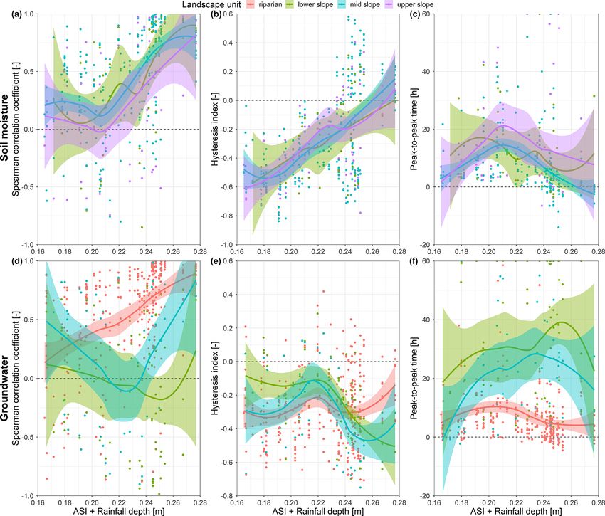
L. Pavlin et al.: Event and seasonal hydrologic connectivity patterns in an agricultural headwater catchment                             2329

Figure 1. Hydrological Open Air Laboratory in Petzenkirchen, Lower Austria. Coloured areas represent different landscape units defined
by the Topographic Position Index (TPI) and terrain slope (riparian zone: TPI ≤ −1; lower slope: −1 < TPI ≤ 0, slope < 5◦ ; mid-slope:
−1 ≤ TPI ≤ 1, slope > 5◦ ; upper slope: TPI > 0, slope ≤ 5◦ ). Elevation contour lines with a 5 m interval are given in black. The inset map is
the detail of the area marked by a black rectangle on the main map.

long-term (2002–2018) average with 736 and 656 mm of                         In the HOAL catchment, a multitude of different runoff
rainfall, respectively. While monthly precipitation peaks in              mechanisms are observed (Blöschl et al., 2016a). Exner-
the summer, monthly runoff tends to peak in winter or early               Kittridge et al. (2016) found that the stream baseflow is
spring when the soil moisture and groundwater levels are                  mostly due to diffuse groundwater flow directly to the stream
highest (Széles et al., 2018).                                            or the springs that feed the stream and partly due to the tile
   The geology of the area consists of Tertiary fine sediments            drainage discharge. During the rainfall events, saturation ex-
of the Molasse underlain by fractured siltstone. Seismic mea-             cess runoff and infiltration excess runoff occur in the valley
surements show that the layer of mostly non-consolidated de-              bottom during prolonged or intensive rainfall events (Silasari
posits is about 200 m thick, except close to the catchment                et al., 2017). Part of the event water enters the stream as an
outlet, where the weathered siltstone lies at a depth of about            overland flow but most infiltrates into the soil matrix and ei-
5 m. Soil core drillings in 2016–2018 show that the pre-                  ther percolates to the groundwater table or is routed to the
dominant soil texture down to 7 m below the surface is silt               stream via tile drains. Macropore flow is observed in summer
loam. Based on double-ring infiltrometer measurements on                  when the topsoil dries and cracks due to the high clay con-
12 plots in our study area, Picciafuoco et al. (2019) deter-              tent (Exner-Kittridge et al., 2016). During rainless periods in
mined a mean saturated hydraulic conductivity of 46.9 and                 the growing season, the diurnal fluctuations of transpiration
20.2 mm h−1 for the topsoil in arable land and grassland, re-             by the riparian vegetation imprint a diurnal fluctuation on the
spectively. The contact to the lignite sequence lies at a depth           streamflow, groundwater levels and soil moisture (Széles et
of 4 to 36 m below the surface. This sequence is a series                 al., 2018).
of dry, low-conductivity, massive and compact lignite lay-
ers interbedded by layers of wet, high-conductivity, and non-             2.2   Data
consolidated sediments with pebbles. Unpublished pumping
test results indicate that these non-consolidated layers have a           There are four OTT Pluvio weighing rain gauges distributed
10–100 times higher hydraulic conductivity than the overly-               throughout the catchment (Fig. 1). They measure precipita-
ing silt loams. Based on a soil survey conducted in 2010, the             tion at 1 min intervals and the differences between the sta-
predominant soil types in the top 1 m are Cambisols (57 %),               tions on the yearly scale do not exceed 5 %. We use the arith-
Kolluvisols (16 %), and Planoslols (21 %). Glaysols (6 %)                 metic mean of precipitation amounts from all four stations as
occur close to the stream (Széles et al., 2018).                          the representative precipitation for the whole catchment.

https://doi.org/10.5194/hess-25-2327-2021                                               Hydrol. Earth Syst. Sci., 25, 2327–2352, 2021
2330       L. Pavlin et al.: Event and seasonal hydrologic connectivity patterns in an agricultural headwater catchment

Table 1. Groundwater (GW) measurement stations in the HOAL used in this study. Distance to the stream and the catchment outlet are the
distances along the surface flowpath from the GW station’s location to the nearest stream reach and catchment outlet, respectively. TWI and
TPI are the topographic wetness and topographic position indices, respectively. The last column shows the number of events when a response
was observed.

          Station    Landscape      Total    Mean     Distance     Distance          TWI           TPI    Local     Days      Number
                     unit           depth     GW         to the       to the          (–)           (–)   slope   without     of event
                                      (m)    depth     stream     catchment                                 (%)      data   responses
                                               (m)         (m)        outlet
                                                                        (m)
          BP01       Riparian        1.12     0.29           1           55      12.89           −2.40     4.68        2           51
          BP02       Riparian        1.13     0.27           1           55      12.89           −2.15     7.75        2           34
          BP07       Riparian        1.59     0.47           1          565      12.57           −3.07     5.60        0           32
          G2         Mid slope      15.00     2.52          76          491       6.89           −0.19    10.21      186           31
          G3         Upper slope    15.00    10.54         330          620       7.81            0.38     0.20       52            0
          G4         Riparian        8.00     1.43          93          676       8.16           −1.55     7.87      110           27
          G8         Upper slope    41.00    28.94         588         1162       5.41            1.27     7.04      108            0
          H01        Lower slope     5.97     4.21          28          287       5.96            0.06    11.22        2           24
          H02        Riparian        2.95     2.64          12          295       6.15           −1.17    13.17        2           32
          H03        Riparian        3.70     0.36           7          296      10.40           −3.44    11.05        2           35
          H04        Riparian        3.50     0.39           1          276      12.68           −3.06     6.69        2           36
          H05        Riparian        3.89     0.17          10          282      13.03           −3.42     4.23        2           37
          H06        Mid slope       3.57     1.08          75          333       7.90            0.02     5.51        2           30
          H07        Lower slope     3.84     1.91          48          306       8.07            0.42     4.51        9           21
          H08        Riparian        2.90     1.75           7          281       8.12           −1.22     8.79        2           27
          H09        Lower slope     3.89     2.57          27          312       7.42           −0.63    10.01        2           14
          H10        Lower slope     4.87     3.04          23          474       7.01           −0.34     9.53        0           10
          H11        Lower slope     4.96     4.46          13          451       4.99           −0.05    14.06        0           17

   Streamflow at the catchment outlet (MW) (Fig. 1) is routed              The soil moisture monitoring network at the study site is
through an H-flume and continuously measured by a Druck                 equipped with Spade time-domain transmission sensors from
PTX1830 submersible pressure transmitter at a 1 min inter-              Forschungszentrum Jülich, Germany, at four depths below
val. There are 18 full days and 12 partial days of missing              the ground surface (5, 10, 20 and 50 cm) (Blöschl et al.,
data in 2017–2018 due to measurement device or data trans-              2016b). For this study, we use 12 permanent stations in the
fer malfunction (Fig. 2).                                               forest, orchards, meadows or field edges and 2 temporary sta-
   We use the measurements from 18 groundwater measure-                 tions in the fields (Fig. 1, Table 2). The temporary stations
ment stations, of which 16 are in and around the forested               are removed and reinstalled twice a year following the agri-
area close to the stream and 2 are at the eastern and north-            cultural practices. Data are collected at an hourly time step.
ern catchment boundaries, respectively (Fig. 1, Table 1). The           Each sensor at each site is calibrated using the gravimetric
stations’ depth is between 1 and 41 m and they are screened             method. We obtain the average volumetric soil moisture over
along the whole depth. Most stations were drilled with a                a depth of 60 cm following Eq. (1):
hammering rig to refusal, which usually corresponds to the
                                                                               4
first consolidated lignite layer’s depth. Exceptions are sta-                  X          di
tions G2, G3, G4 and G8, which were drilled into but not                θ=           θi      ,                                           (1)
                                                                               i=1
                                                                                          D
through all the lignite layers. All stations are equipped with
pressure water level loggers by vanEssen, with a resolution             where θ is the mean volumetric soil moisture content; θi is
of 0.1 cm H2 O and typical accuracy of 0.5 cm H2 O, which               the volumetric soil moisture content at ith sensor and D is the
measure at 5 min time intervals. Water level loggers’ mea-              soil column depth (60 cm). di is representative column height
surements are barometrically compensated using the atmo-                of the ith sensor determined as the distance between mid-
spheric pressure measured by Baro Diver by vanEssen lo-                 points to the sensor above and below the ith sensor (e.g. d1
cated close to H11 (Fig. 1). Stations G3, G4 and G8 were                to d4 are 7.5, 7.5, 20 and 25 cm). Representative columns
only installed in February 2017 and G2 in July 2017, but                of the top-most and bottom-most sensors extend up to the
they are used in the study due to their locations outside the           ground surface and down to D, respectively. If measurements
forested area. Other stations only have missing data from 4 to          from one or two sensors are missing, the di are adjusted so
7 December 2018 due to measurement device failure (Fig. 2).             that working sensors represent more of the soil column.

Hydrol. Earth Syst. Sci., 25, 2327–2352, 2021                                                    https://doi.org/10.5194/hess-25-2327-2021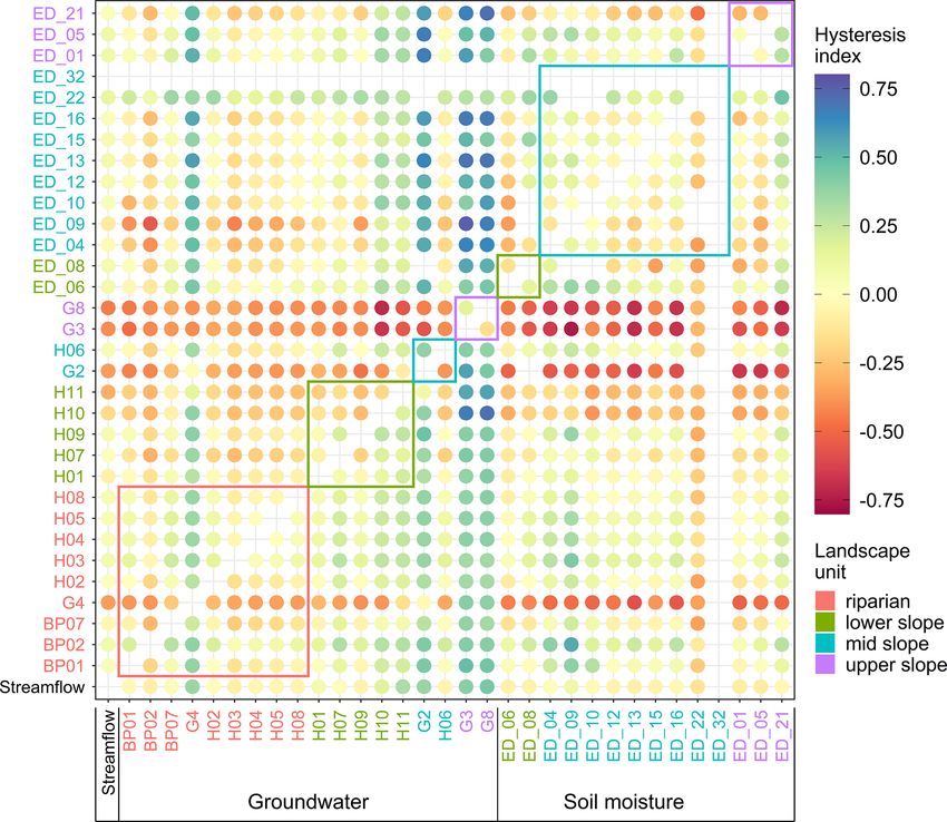
L. Pavlin et al.: Event and seasonal hydrologic connectivity patterns in an agricultural headwater catchment                        2331

Figure 2. Dynamics of rainfall, streamflow at the catchment outlet, antecedent soil moisture index (ASI), groundwater (BP01, G4, H06, H07)
and soil moisture (ED_21) during the investigation period, 2017–2018. The shaded areas represent the times of analysed events.

   For this study, we use the streamflow at the catchment              most of the peak-to-peak lag times were of orders of hours
outlet, groundwater levels, precipitation and soil moisture            (see Sect. 3.1.1). We further aggregate the dataset to median
data from 2017 and 2018. We average the groundwater and                weekly values to dampen the event dynamics for the analysis
streamflow data with the 5 min time step to the 15 min time            of the seasonal scale. We choose the weekly time step as it is
step and linearly interpolate the soil moisture data from 1 h          longer than any observed event.
to the 15 min time step. This time step is small enough to
capture the quick responses of streamflow, groundwater, and            2.3   Site characteristics
soil moisture to the precipitation. The streamflow, groundwa-
ter levels and soil moisture data are additionally smoothed            To put groundwater and soil moisture responses into the
using the locally estimated scatterplot smoothing (LOESS)              catchment’s spatial context, we derive various site charac-
as implemented in the R programming language stats pack-               teristics based on the sites’ position and the digital eleva-
age (R Core Team, 2019). This step smooths out the mea-                tion model (DEM) with 1 m resolution smoothed with a 10 m
surement noise and eases the peak detection, which is based            by 10 m box filter. For the calculations, we use SAGA GIS
on the search for time steps in the time series preceded by            (Conrad et al., 2015). First, the local slope and general cur-
consecutive rising and succeeded by consecutive decreasing             vature of the topography are calculated. Upslope catchment
values. Smoothing might have shifted the peak time by one              area and surface flowpaths are determined from the DEM by
time step in some cases, which we deem acceptable since                the multiple flow direction method (Freeman, 1991). The dis-

https://doi.org/10.5194/hess-25-2327-2021                                            Hydrol. Earth Syst. Sci., 25, 2327–2352, 2021
2332        L. Pavlin et al.: Event and seasonal hydrologic connectivity patterns in an agricultural headwater catchment

Table 2. Soil moisture (SM) measurement stations and their properties. ∗ denotes a temporary station. Distance to the stream and the
catchment outlet are the distances along the surface flowpath from the SM station’s location to the nearest stream reach and catchment outlet,
respectively. TWI and TPI are the topographic wetness and topographic position index, respectively. The last column shows the number of
events when a response was observed.

                   Station     Landscape       Distance     Distance      TWI        TPI    Local      Days      Number
                               unit               to the       to the      (–)        (–)   slope    without     of event
                                                stream     catchment                          (%)       data    responses
                                                    (m)        outlet
                                                                 (m)
                   ED_01       Upper slope         1250         1840      5.91     0.72      4.09         62        24
                   ED_04       Mid slope            911         1476      6.08     0.28      8.17        316        36
                   ED_05       Upper slope          613         1189      5.35     1.26      3.70         74        20
                   ED_06       Lower slope          433         1012     11.56    −0.14      2.65        331        28
                   ED_08       Lower slope          213          792      9.29    −0.43      2.35         44        22
                   ED_09       Mid slope            353          927      6.72     0.25     11.28         41        14
                   ED_10∗      Mid slope            181          597      7.57    −0.31      4.48         22        33
                   ED_12       Mid slope            238          533      6.00     0.64      4.14        161        35
                   ED_13       Mid slope             91          569      7.29    −0.65      8.79        127        32
                   ED_15       Mid slope             81          314      7.59     0.15      5.51         95        40
                   ED_16       Mid slope            175          257      4.76     1.15     20.26        112        27
                   ED_21       Upper slope          356          937      6.78     0.69      4.91         33        29
                   ED_22       Mid slope            325          888      6.01     0.66      4.21         68        18
                   ED_32∗      Mid slope             61          290      6.74     0.43      7.12         51        16

tance along the surface flowpath from each of the ground-                with a rainfall depth of at least 1 mm starts. Selected reces-
water and soil moisture stations to the nearest stream reach             sion time covers most of the groundwater event dynamics
and the catchment outlet is then calculated. The topographic             while minimizing the coverage of the stream baseflow fluctu-
control on local drainage is quantified by the Topographic               ations; (5) no threshold is imposed on streamflow. However,
Wetness Index (TWI) (Beven and Kirkby, 1979), which is                   no streamflow data should be missing during the duration of
calculated by the SAGA wetness index (Böhner and Selige,                 the rainfall-runoff event; (6) at least one groundwater or soil
2006) module in SAGA GIS.                                                moisture response is found (Sect. 2.5).
   Slope position is quantified by the Topographic Position                 For each event, we calculate the following event charac-
Index (TPI) (Weiss, 2001). The TPI compares the elevation                teristics. The event duration is the total time between the
of a point and the mean elevation of its surroundings. Points            start and end of the event, as defined above. Rainfall event
in the valleys have negative and points on the ridges posi-              duration is calculated as time elapsed from the beginning
tive TPI values. The TPI can be used for the classification              of the event until 90 % of the rainfall amount fell. Rain-
of the landscape into slope position units. We classify our              fall depth is the sum of all precipitation that occurred dur-
study site with the TPI Based Landform Classification tool               ing the event. The maximum rainfall intensity is the maxi-
in SAGA GIS into four position classes: riparian zone, lower             mum rainfall amount per 15 min interval during the whole
slope, mid slope and upper slope (Fig. 1), with mean TPI val-            event. Change in streamflow (dQ) is the difference between
ues of −2.0, −0.4, 0 and 0.5 and mean slope values of 7.5,               the maximum and minimum streamflow during the event.
5.0, 6.5 and 4.2◦ , respectively.                                        The streamflow peak time is the elapsed time from the be-
                                                                         ginning of the event until streamflow reaches its maximum.
2.4    Rainfall-runoff event definition and                              The runoff depth is the sum of the streamflow, reduced by
       characterization                                                  its minimum, multiplied by the time step (15 min) and di-
                                                                         vided by the catchment area (66 ha). Following Saffarpour et
We identify 53 rainfall-runoff events during 2017 and 2018               al. (2016), we use the antecedent soil moisture index (ASI)
(Fig. 2) that meet all of the following six conditions: (1) sig-         to measure catchment wetness. We calculate it as the mean
nificant rainfall is more than 0.1 mm in 15 min; (2) rainfall            volumetric soil moisture content of all soil moisture stations
events are separated by a period of at least 6 h when no signif-         over 24 h before the start of an event multiplied by the soil
icant rainfall occurs; (3) a rainfall event must have the rainfall       column depth (0.6 m). A table of all events and their charac-
depth of at least 4 mm; (4) the rainfall-runoff event starts with        teristics is in the Appendix (Table A1).
the rainfall event but continues after the rainfall has stopped
for a recession period of 48 h or until a new rainfall event

Hydrol. Earth Syst. Sci., 25, 2327–2352, 2021                                               https://doi.org/10.5194/hess-25-2327-2021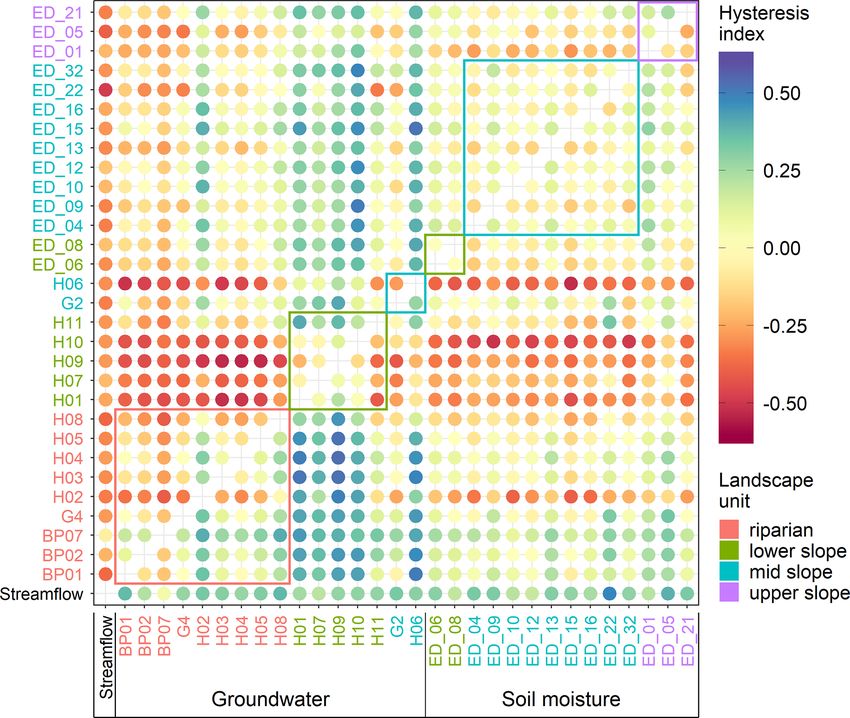
L. Pavlin et al.: Event and seasonal hydrologic connectivity patterns in an agricultural headwater catchment                       2333

Figure 3. Time series of streamflow at the catchment outlet, rainfall (a, b) and groundwater table (BP01, G4, H06, H07) and soil moisture
content (ED_21) (c, d) difference from the event minimum during event 29 (a, c) and event 44 (b, d). P and ASI denote the rainfall depth
and antecedent soil moisture index of each of the events, respectively.

2.5   Groundwater and soil moisture event response                     tions and 374 soil moisture responses at 14 stations. We
      definition and characterization                                  adopt three event descriptors: Spearman correlation coeffi-
                                                                       cient, hysteresis index, and peak-to-peak time for the com-
                                                                       parison of these responses. We choose these three because
We determine whether the groundwater or soil moisture at
                                                                       they are easy to understand, suitable for all variables whose
a station reacted to the precipitation event based on the
                                                                       responses are due to the same driver and transferable to other
following rules: (1) stations’ event time series must not
                                                                       catchments.
monotonously rise (Fig. 3d, station H06) or recede (Fig. 3d,
                                                                          Hysteresis loops have been demonstrated as a simple but
station H07), must not be masked by a diurnal signal (Fig. 3d,
                                                                       insightful method for investigating the relationships between
station BP01) and must have a peak (Fig. 3c). The peak is a
                                                                       streamflow and other hydrological or chemical variables
point in the time series preceded by at least 24 time steps
                                                                       (Allen et al., 2010; Fovet et al., 2015; Scheliga et al., 2018).
of increasing and at least 4 time steps of decreasing values.
                                                                       We can obtain a hysteresis loop if we plot concurrent values
If more peaks are detected, the one closest to the time of
                                                                       of two variables against each other. The hysteresis index (HI)
the streamflow peak is selected. (2) The minimum change
                                                                       describes the size and rotational direction of such a loop. Var-
in the groundwater table and soil moisture content is 5 mm
                                                                       ious definitions of the HI have been proposed in hydrology
and 0.005 m3 m−3 , respectively. The change is calculated as
                                                                       (Aich et al., 2014; Langlois et al., 2005; Lawler et al., 2006;
the difference between the value at the peak and the mini-
                                                                       Lloyd et al., 2016; Zuecco et al., 2016). In this study, we
mal value before it. We also determine local antecedent con-
                                                                       use a definition similar to Lloyd et al. (2016) and Zuecco et
ditions as the mean groundwater table or soil moisture 1 h
                                                                       al. (2016). The input time series (e.g. streamflow, ground-
before the event for each response.
                                                                       water level, soil moisture) are first normalized to values be-
   During the 53 rainfall-runoff events, we observed a total
                                                                       tween 0 and 1 by the range of values for a specific event. The
of 458 groundwater responses to the precipitation at 15 sta-

https://doi.org/10.5194/hess-25-2327-2021                                            Hydrol. Earth Syst. Sci., 25, 2327–2352, 2021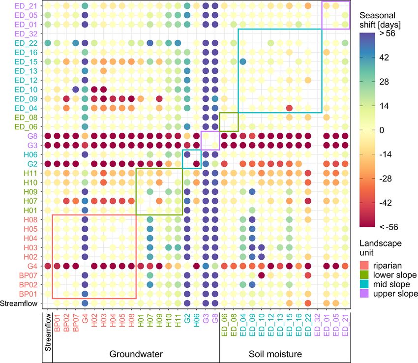
2334       L. Pavlin et al.: Event and seasonal hydrologic connectivity patterns in an agricultural headwater catchment

Figure 4. Weekly median time series of streamflow at the catchment outlet (MW) and the groundwater table (BP01, G4, H06, H07) and the
soil moisture content (ED_21) difference from the minimum for the years 2017–2018.

HI is then calculated as the integral of the loop of the two         all events and both years. We investigate the temporal pat-
normalized variables plotted against each other. The resulting       terns in terms of changing wetness conditions, which can
HI ranges between −1 and 1, where the magnitude describes            only be done on the event scale. For that, we use the com-
the loop’s shape and the sign the rotational orientation. The        parisons of groundwater and soil moisture event responses to
wider the loop, the greater the absolute HI value. Clockwise         streamflow and aggregate them by landscape units and the
loops, where the variable on the vertical axis peaks first, have     sum of ASI and total rainfall. The entire analysis is done
positive HI values. The anticlockwise loops, where the vari-         with the R programming language (R Core Team, 2019). Sta-
able on the horizontal axis peaks first, have negative HI val-       tistical significance is assessed by p values calculated using
ues. A detailed explanation of the HI calculation is in Ap-          the t-distribution approximation as implemented in the stats
pendix B.                                                            package.
   Peak-to-peak time is the time difference between the peak
time of the first and second variables. Peak-to-peak times to        2.6   Classification of event responses
streamflow are positive if the streamflow peaks first and neg-
ative if the other variable peaks first.                             To investigate the control of site and event characteristics
   To describe the similarity between streamflow, groundwa-          on the connectivity on the event scale, we first classify the
ter and soil moisture seasonal dynamics, we also use three           relationship between the streamflow event response to the
descriptors, i.e. Spearman correlation coefficient, hysteresis       groundwater and soil moisture event response into response
index and time shift in seasonal dynamics. The latter dif-           types. The classification is based on the event descriptors
fers from the peak-to-peak time calculated on the event scale.       (Spearman correlation coefficient, hysteresis index and peak-
Seasonal time shift is the lag time when the cross-correlation       to-peak time) and performed by combining the hierarchi-
of two variables is the highest. For these calculations, the         cal clustering analysis and classification trees. An additional
weekly median of streamflow, groundwater levels and soil             benefit of response types compared to the adopted descrip-
moisture content are used to smooth out the event dynamics           tors is potentially better transferability to other catchments
(Fig. 4). Only stations with more than 45 weeks of data in a         with for example more conductive soils.
year are used. Because of data gaps, station ED_32 is left out          Hierarchical clustering is a method of identifying groups
entirely, stations G2–G4, ED_09 and ED_10 are left out for           of similar data points in a dataset. We use the descriptors
the year 2017 and stations ED_08 and ED_22 are left out for          mentioned above of groundwater event responses from all
the year 2018.                                                       observed events at all available stations as the input dataset
   For the analysis of spatial patterns, we calculated the me-       variables. Only groundwater responses are used in this step
dian value of the three descriptors for each station pair over       because they have greater variability of descriptor values
                                                                     than soil moisture responses. The clustering is performed

Hydrol. Earth Syst. Sci., 25, 2327–2352, 2021                                         https://doi.org/10.5194/hess-25-2327-2021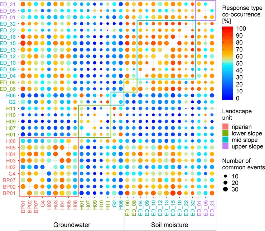
L. Pavlin et al.: Event and seasonal hydrologic connectivity patterns in an agricultural headwater catchment 2335
Figure 5. Decision tree for the classification of groundwater re-
sponses in relation to the streamflow responses to precipitation
events into three response types. Responses are split based on the
hysteresis index (HI) and Spearman correlation coefficient (Cor), as
shown by the expressions on the horizontal lines between nodes.
Each node is coloured based on the predominant response type,
while the colour intensity denotes the purity of the classification.
Node text shows the predominant response type, the percent of re- Figure 6. Median Spearman correlation coefficient between stream-
sponses of each type at that node in the input database (IN) and the flow at catchment outlet (streamflow), groundwater stations (BP∗ ,
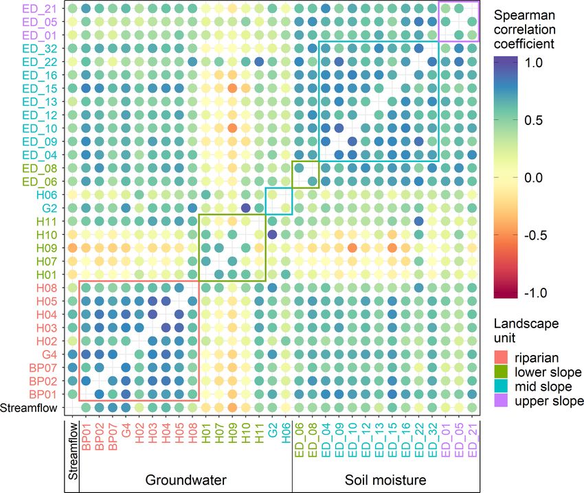
percent of the total number of responses at that node (OUT). H∗∗ , G∗ ) and soil moisture stations (ED_∗∗ ) for all events. The cir-
cles’ colour corresponds to the Spearman correlation coefficient.
The station names’ colour corresponds to their landscape unit.
with Ward’s hierarchical clustering algorithm (Murtagh and Coloured rectangles enclose correlations of stations in the same
landscape unit.
Legendre, 2014) implemented in the stats package in the
R programming language (R Core Team, 2019), which gives
us three clusters of similar size.
3 Results
A disadvantage of hierarchical clustering is a lack of spe-
cific rules that could be used to classify additional hydrolog- 3.1 The similarity of groundwater, soil moisture and
ical variables or datasets from other catchments. That is why streamflow event responses
we do an extra step and use the information gained from clus-
tering to construct a discrete decision tree, also known as a 3.1.1 Spatial patterns
classification tree. The cluster number is used as a dependent
and the three event descriptors are used as independent vari- We find spatial patterns in the median event Spearman
ables in the input dataset for the classification tree algorithm correlation coefficients between groundwater responses and
implemented in R package rpart (Therneau and Atkinson, streamflow response (Fig. 6). The riparian stations BP01,
2019). The resulting three-node classification tree is shown BP02, BP07, H04, H05 and G4 have the highest mean Spear-
in Fig. 5. It allows us to determine the type of relationship man correlation with the streamflow (rs > 0.6). Correlation
between two responses with the precipitation event, based is lower in other groundwater stations. All of the soil mois-
only on the hysteresis index and Spearman correlation coef- ture stations have mostly moderate correlations with stream-
ficient. The difference between the response type determined flow (0.3 < rs < 0.5). The similarity among the stations in
by the clustering and by the classification tree is less than the same landscape unit is comparable to the similarity to
6 %. This classification tree is also used here to classify the streamflow. The riparian zone groundwater stations (Fig. 6,
soil moisture responses to precipitation events in relation to red rectangle) have the highest Spearman correlation co-
streamflow. efficients among them (rs = 0.75). Correlations among the
We assess how site and event characteristics affect the con- lower-slope and mid-slope stations are lower, and they are
nectivity on the event scale by looking at how they correlate also not well correlated with other stations. Exceptions are
with response types. We calculate the Pearson correlation co- station H11, positioned above the stream valley, but it is
efficient between each response type’s frequency to the site very close to the stream, and station G2, located far from
characteristics of each station. We also calculate the correla- the stream but in an always wet location. Overall, the soil
tion between each response type’s frequency for each event moisture stations are well correlated among themselves (rs =
to the event characteristics for groundwater and soil moisture 0.69) and moderately correlated with the riparian groundwa-
stations. We deem correlations with p < 0.05 to be signifi- ter stations. Upper-slope soil moisture stations have a lower
cant. correlation among them and with other stations compared to
the average for the soil moisture stations.
https://doi.org/10.5194/hess-25-2327-2021 Hydrol. Earth Syst. Sci., 25, 2327–2352, 2021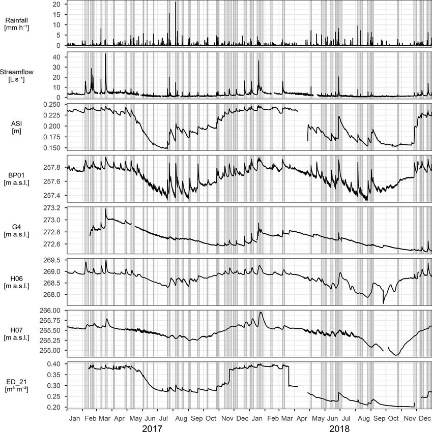
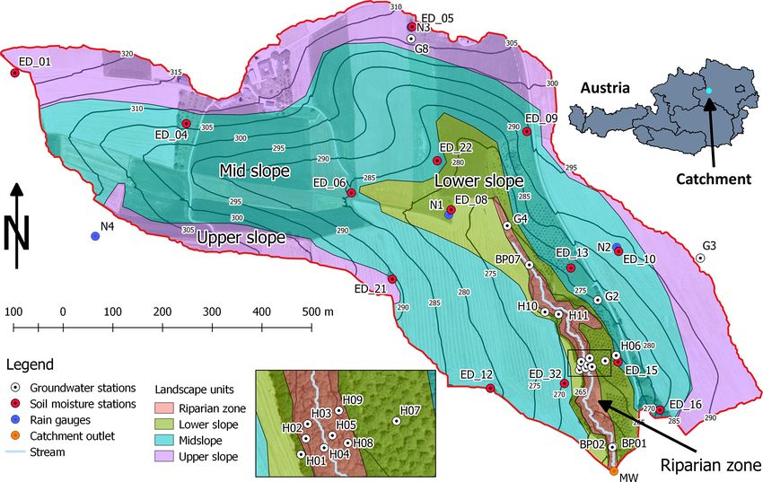
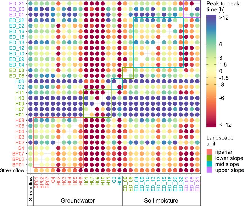
2336        L. Pavlin et al.: Event and seasonal hydrologic connectivity patterns in an agricultural headwater catchment

Figure 7. Median hysteresis index between streamflow at catch-          Figure 8. Median peak-to-peak time between streamflow at catch-
ment outlet (streamflow), groundwater (BP∗∗ , H∗∗ , G∗ ) and soil       ment outlet (streamflow), groundwater (BP∗∗ , H∗∗ , G∗ ) and soil
moisture (ED_∗∗ ) for all events. Hysteresis index is positive if the   moisture (ED_∗∗ ). Time is positive if the row station peaks be-
row station peaks before the column station and negative if the row     fore the column station and negative if the row station peaks after
station peaks after the column station. Circles’ colour corresponds     the column station. Circles’ colour corresponds to the value of the
to the value of the hysteresis index. The station names’ colour cor-    peak-to-peak time. The station names’ colour corresponds to their
responds to their landscape unit. Coloured rectangles enclose values    landscape unit. Coloured rectangles enclose values of stations in the
of stations in the same landscape unit.                                 same landscape unit.

   The median event hysteresis indices between streamflow,
groundwater and soil moisture event responses show similar              There, in some instances, groundwater even peaked before
spatial patterns (Fig. 7) as the median event Spearman cor-             streamflow (Figs. A1c and 9f). The Pearson correlation coef-
relation coefficient. Where the Spearman correlation coeffi-            ficient between the event response Spearman correlation co-
cient is high, the hysteresis index is closer to zero, and where        efficient and TWI (Fig. A1a) and TPI is ρ = 0.38 and ρ =
the coefficient is low, the absolute value of the hysteresis in-        −0.45, respectively. Pearson correlation coefficient between
dex is high. Most of the hysteresis indices of groundwater              the peak-to-peak time and TWI (Fig. A1c) and TPI is ρ =
and soil moisture responses against streamflow responses are            −0.42 and ρ = 0.51, respectively. In other words, ground-
negative (Fig. 7, first column). This indicates that, on aver-          water event responses towards the valley bottom, where the
age, the hysteresis loops are anticlockwise and streamflow              contributing area is greater and the groundwater table is shal-
responds to precipitation (Fig. 8, first column) quicker than           lower, are increasingly more similar to the streamflow re-
groundwater and soil moisture do.                                       sponses. The peak-to-peak times between them are decreas-
   Spatial patterns in median event peak-to-peak times                  ing. The soil moisture event response descriptors do not cor-
(Fig. 8) confirm the assessment based on the hysteresis in-             relate with the site characteristics (Fig. A1).
dex (Fig. 7, first column). On average, groundwater and soil
moisture peak later than streamflow. Further, Fig. 8 reveals            3.1.2   Temporal patterns through wetness conditions
details that are not so clearly visible in the median event cor-
relation and hysteresis index. The upper-slope soil moisture            While there is small spatial variability of descriptors for soil
stations peak later than other soil moisture stations. We see           moisture responses in relation to the streamflow, the pattern
also that groundwater stations H02 and H08 are different to             changes in time with the catchment wetness (ASI + rainfall
the rest of the riparian stations and are more like the lower-          depth) (Fig. 9, top row). Spearman correlation coefficient
slope stations, which is probably due to their deeper ground-           and the hysteresis index increase with the increasing wetness
water table compared to the rest of the riparian stations.              (Pearson correlation of ρ = 0.45 and ρ = 0.57, respectively).
   On average, groundwater and soil moisture at all stations            The trend of peak-to-peak time is nonlinear in the shape of an
peak 15 ± 21 and 9 ± 14 h (mean and standard deviation) af-             inverted parabola (Fig. 9c), with the longest times at medium
ter streamflow, respectively (Fig. 8, first column). The low-           wetness conditions. These three trends are very similar for all
est peak-to-peak times between streamflow and groundwa-                 landscape units. The small dip in correlation and increase in
ter were observed in the riparian zone (median 2.7 ± 14 h).             peak-to-peak times during medium wetness conditions might

Hydrol. Earth Syst. Sci., 25, 2327–2352, 2021                                             https://doi.org/10.5194/hess-25-2327-2021
L. Pavlin et al.: Event and seasonal hydrologic connectivity patterns in an agricultural headwater catchment                              2337

Figure 9. Spearman correlation coefficient (a, d), hysteresis index (b, e) and peak-to-peak time (c, f) of soil moisture (a–c) and groundwa-
ter (d–f) responses to streamflow event responses over changing event catchment wetness conditions (ASI + rainfall depth). Colours represent
different landscape units. Points are calculated values for each available response. Lines are local regression fits for each landscape unit and
shaded areas the corresponding 95 % confidence intervals.

indicate that different flowpaths activate during the dry and             to-peak time suggest that the control of the wetness condi-
wet conditions.                                                           tions is related to the mean groundwater depth in the land-
   Trends of groundwater event response descriptors with the              scape unit. Trends are the clearest in the riparian zone, where
wetness conditions differ for each landscape unit (Fig. 9, bot-           the groundwater table is the shallowest, followed by the mid
tom row). Spearman correlation coefficient steadily increases             slope and lower slope, which has the deepest groundwater
with increasing wetness in the riparian zone (Fig. 9d). At                table.
the same time, there is no clear trend in the lower slope                    In the vast majority of cases, groundwater peaks after the
and a parabolic trend in the mid slope, probably due to a                 streamflow (Fig. 9). During wet conditions (ASI + rainfall
deeper groundwater table. Trends of hysteresis index and                  depth > 0.23), there are many stations in the riparian zone
peak-to-peak time are not so clear. Peak-to-peak times are                that peak before. This difference probably indicates that most
shorter in the riparian zone compared to other landscape                  of the time, flowpaths bypassing the groundwater (monitor-
units. They also seem to shorten with the increasing wetness,             ing stations) feed the event streamflow. Only when the catch-
which is coherent with the increasing correlation. Peak-to-               ment wetness is sufficiently high does the riparian zone con-
peak times in the mid slope are lower than in the lower slope,            tribute to the event streamflow.
which is again coherent with the Spearman correlation coef-
ficient. Trends of Spearman correlation coefficient and peak-

https://doi.org/10.5194/hess-25-2327-2021                                                Hydrol. Earth Syst. Sci., 25, 2327–2352, 2021
2338        L. Pavlin et al.: Event and seasonal hydrologic connectivity patterns in an agricultural headwater catchment

Figure 10. Hysteresis loops for event 29 (31 December 2017)
(Fig. 3c). Each panel represents a different response type: (a) type-
1 groundwater (GW) response; (b) type-2 GW response; (c) type-          Figure 11. The frequency of events when two stations have the re-
3 GW response; (d) type-1 soil moisture (SM) response. The points’      sponse of the same type – i.e. response-type co-occurrence. The
colour represents the time since the start of the event. Event dynam-   size of circles corresponds to the number of events when both sta-
ics of each station in relation to the streamflow is described by the   tions had a response. Circles’ colour corresponds to the frequency
response type (Type), peak-to-peak time (Lag), Spearman correla-        of the response-type co-occurrence. The station names’ colour cor-
tion coefficient (Cor), hysteresis index (HI) and groundwater table     responds to their landscape unit. Coloured rectangles enclose values
or soil moisture content change over the event (1h).                    of stations in the same landscape unit.

3.2     Event response types                                                 −0.98 and 0. These groundwater and soil moisture re-
                                                                             sponses were least correlated with streamflow. Their ris-
3.2.1    Event response classification                                       ing limb either started late after the start of the rain-
                                                                             fall or continued to increase past the end of event time
Altogether we determined 170, 203 and 85 groundwater re-
                                                                             (Fig. 10c).
sponses and 136, 183 and 55 soil moisture responses in re-
lation to the streamflow of type 1, type 2 and type 3, respec-          3.2.2   Spatial patterns of event response types
tively. Response types represent different levels of similarity
between the groundwater or soil moisture to the streamflow,             The spatial patterns of hysteresis index, Spearman correla-
as follows.                                                             tion coefficient and peak-to-peak times (Sect. 3.1.1) prop-
                                                                        agate to the pattern of event response type co-occurrence
  – Type-1 responses have a hysteresis index between −0.3
                                                                        (Fig. 11). Event response type co-occurrence is the frequency
    and 0.58 and a Spearman correlation coefficient be-
                                                                        of events when two stations have the same type of response.
    tween 0 and 0.99. These were groundwater and soil
                                                                        Apart from the riparian zone, where the co-occurrence rate
    moisture responses that were similar to the stream-
                                                                        is 64 % ± 15 % between stations, the other two landscape
    flow response. The hysteresis loop was narrow, the lag
                                                                        units show only low co-occurrence rates of groundwater re-
    time was short, and the groundwater table or soil mois-
                                                                        sponse types between stations in the same unit. The highest
    ture content have increased and decreased on the same
                                                                        co-occurrence rate is observed between the three piezome-
    timescale as the discharge (Fig. 10a and d).
                                                                        ters H03, H04 and H05. These stations respond with the same
  – Type-2 responses had a hysteresis index between −0.84               response type in more than 85 % of the events. Their co-
    and −0.3 and a correlation coefficient between −0.2                 occurrence rate with piezometers downstream (BP01, BP02)
    and 0.96. Typical for these response types are wide hys-            and upstream (BP07) is also high (68 %–84 %), indicating
    teresis loops. The rising limb of the groundwater or soil           that the distance to the stream is more important than the
    moisture event time series is relatively long but still             position along the stream. Riparian zone piezometers have
    overlaps with the streamflow hydrograph’s rising and                a reasonable response type co-occurrence rate with the soil
    receding limb (Fig. 10b).                                           moisture stations (62 % ± 14 %). Soil moisture stations, with
                                                                        some exceptions, have high co-occurrence rates regardless of
  – Type-3 responses either had a hysteresis index between              the landscape unit (mean 78 % ± 11 %).
    −0.64 and 0.16 or a correlation coefficient between

Hydrol. Earth Syst. Sci., 25, 2327–2352, 2021                                             https://doi.org/10.5194/hess-25-2327-2021
L. Pavlin et al.: Event and seasonal hydrologic connectivity patterns in an agricultural headwater catchment 2339
Figure 12. Seasonal hysteresis loops of three groundwater sta-
tions (a–c) and one soil moisture station (d) to the streamflow for the Figure 13. Median Spearman correlation coefficient between me-
year 2018 (Fig. 4). Circles’ colour represents the week of the year. dian weekly streamflow at catchment outlet (Q), groundwater
Seasonal dynamics of each station in relation to the streamflow is (BP∗∗ , H∗∗ , G∗ ) and soil moisture (ED_∗∗ ) over years 2017
described by seasonal shift (Lag), Spearman correlation (Cor), hys- and 2018. Circles’ colour corresponds to the value of the Spearman
teresis index (HI) and groundwater table elevation or soil moisture correlation coefficient. The station names’ colour corresponds to
content change over the year (1h). their landscape unit. Coloured rectangles enclose values of stations
in the same landscape unit. Only time series longer than 45 weeks
per year are compared.
3.2.3 Spatial and temporal controls of event response
types
are correlated with the rainfall duration (Table 3). The re-
sponses are more similar to streamflow when the events are
We observe the clearest trend in the groundwater response- longer, i.e. less intensive.
type frequency with the TPI and the TWI (Table 3). The fre-
quency of the type-1 responses decreases, and the frequency 3.3 Similarity of groundwater, soil moisture and
of the type-3 responses increases with the TPI increase and streamflow seasonal dynamics
the TWI decrease (Fig. A2a). This trend means that ground-
water in the valley bottom reacts more like streamflow than Examples of the seasonal hysteresis loops of the stations G4,
on the slopes and ridges. The response-type frequency by H06, H07 and ED_21 are shown in Fig. 12. Shapes of loops
landscape units further corroborates this result. The type-1 in Fig. 12a–c are different from corresponding event loops
frequency is more than 43 % in the riparian zone and only in Fig. 10, indicating a difference in the similarity in the
22 % and 18 % in the lower and mid slopes, respectively. The seasonal and event dynamics of these stations to the stream-
highest frequency of type-3 responses is at the lower slope flow. We see further differences between the median seasonal
(50 %), while it is lowest in the riparian zone (7 %). The soil Spearman correlation coefficients (Fig. 13), hysteresis index
moisture response-type frequencies do not vary considerably (Fig. 14) and time shift (Fig. 15) to their counterparts on the
with the TPI or the TWI (Fig. A3a) but rather with the dis- event scale (Figs. 6–8).
tance from the stream and the catchment outlet and less pro- The Spearman correlation coefficient of groundwater and
nounced with the terrain curvature and slope (Table 3). Soil soil moisture seasonal dynamics to the streamflow (Fig. 13)
moisture responses are less similar, i.e. frequency of type-3 is, in contrast to the event scale, high (ρ > 0.7) for all sta-
increases, further from the stream or catchment outlet and tions except G2 (ρ = 0.63), G3 (ρ = 0.14), G4 (ρ = 0.63)
where the curvature and slope of the terrain are smaller. and G8 (ρ = 0.07). Surprisingly, the lower- and mid-slope
Soil moisture response-type frequencies are correlated the groundwater stations with a low correlation with streamflow
strongest with the catchment wetness (ASI, ASI + rainfall on the event scale show a high correlation on the seasonal
depth) (Table 3). With increasing wetness, the similarity scale. Two examples are stations H01 and H06, with mean
of soil moisture responses to the streamflow also increases event correlations with streamflow of ρ = −0.15 and ρ =
(Fig. A3b). This correlation is weaker for the frequency of −0.04 and seasonal correlations of ρ = 0.93 and ρ = 0.89,
groundwater response types. The frequencies of both ground- respectively. Correlation among stations in the same land-
water (Fig. A2c) and soil moisture (Fig. A3c) response types scape unit is highest in the riparian zone, also on the seasonal
https://doi.org/10.5194/hess-25-2327-2021 Hydrol. Earth Syst. Sci., 25, 2327–2352, 20212340 L. Pavlin et al.: Event and seasonal hydrologic connectivity patterns in an agricultural headwater catchment
Table 3. Pearson correlation coefficient of site and event characteristics with the frequency of different event response types of groundwater
and soil moisture in relation to the streamflow. ASI is the antecedent soil moisture index. TPI and TWI are topographic position index and
topographic wetness index, respectively. The significance of correlations was tested with t-distribution approximation and correlations with
p < 0.05 are shown in bold.
Groundwater responses Soil moisture responses
Response type Type 1 Type 2 Type 3 Type 1 Type 2 Type 3
Event characteristics
ASI 0.03 −0.03 –0.38 0.67 −0.24 −0.39
ASI + rainfall depth 0.09 −0.14 –0.47 0.70 –0.38 −0.40
Rainfall duration 0.31 –0.34 –0.40 0.47 –0.50 −0.01
Maximum rainfall intensity −0.01 −0.17 0.32 –0.39 0.14 −0.03
Rainfall depth 0.15 –0.31 −0.18 0.05 –0.31 0.03
Site characteristics
Distance to the outlet 0.35 −0.13 0.17 −0.24 −0.27 0.59
Distance to the stream 0.03 −0.08 0.33 −0.11 −0.34 0.52
Curvature −0.29 0.31 −0.11 −0.09 0.26 −0.35
Slope −0.24 0.14 −0.02 0.11 0.28 −0.34
Upslope area 0.36 0.18 −0.39 0.05 −0.01 −0.05
TPI –0.57 −0.31 0.64 −0.02 −0.08 0.10
TWI 0.56 0.10 −0.48 0.10 −0.02 −0.09
Mean groundwater depth 0.43 0.20 −0.39 – – –
scale. Still, the difference to other landscape units is smaller
compared to the event scale. Even upper-slope groundwa-
ter stations, which do not correlate well with stations in
other landscape units, are well correlated with each other.
All soil moisture stations are well correlated with the stream
(rS = 0.83 ± 0.06) and among them in all landscape units.
The seasonal- and event-scale patterns are more similar
for the median hysteresis index (Fig. 14) than the Spearman
correlation coefficient. Riparian station G4 and some lower-,
mid- and upper-slope groundwater stations have a negative
hysteresis index against the streamflow (Fig. 14, first col-
umn), indicating a delay in their seasonal dynamics. These
are stations with the deepest groundwater table, and some
are also in contact with the deep groundwater system. All
soil moisture stations have a hysteresis index in relation to
the streamflow close to zero or even slightly positive, indi-
cating mostly synchronous seasonal dynamics.
Seasonal dynamics of streamflow, groundwater and soil
moisture in the research area is roughly sinusoidal, with the
highest values in winter and the lowest in summer. The sea-
Figure 14. Median hysteresis index between median weekly sonal dynamics shift time tells us how much out of phase the
streamflow at catchment outlet (Q), groundwater (BP∗∗ , H∗∗ , G∗ ) dynamics of two stations are. Figure 15 shows that the dy-
and soil moisture (ED_∗∗ ) over the years 2017 and 2018. Hysteresis
namics of stations G2, G3, G4 and G8 are delayed compared
index is positive if the row station peaks before the column station
and negative if the row station peaks after the column station. Cir-
to the streamflow by 56, 91, 49 and 70 d, respectively. On the
cles’ colour corresponds to the value of the hysteresis index. The other hand, some soil moisture stations show slightly early
station names’ colour corresponds to their landscape unit. Coloured dynamics, which indicates that soil moisture conditions drive
rectangles enclose values of stations in the same landscape unit. the seasonal dynamics of streamflow and partly groundwater.
Only time series longer than 45 weeks per year are compared. The spatial homogeneity of the seasonal soil moisture dy-
namics is reflected in a weak correlation between the site
Hydrol. Earth Syst. Sci., 25, 2327–2352, 2021 https://doi.org/10.5194/hess-25-2327-2021L. Pavlin et al.: Event and seasonal hydrologic connectivity patterns in an agricultural headwater catchment 2341
Table 4. Pearson correlation coefficient between site characteristics and the Spearman correlation, hysteresis index and time shift of ground-
water and soil moisture seasonal dynamics in relation to streamflow. TPI and TWI are topographic position index and topographic wetness
index, respectively. Significance of correlations was tested with t-distribution approximation and correlations with p < 0.05 are shown in
bold.
Groundwater Soil moisture
Descriptor Spearman Hysteresis Shift in Spearman Hysteresis Shift in
correlation index dynamics correlation index dynamics
Site characteristics
Distance to the outlet –0.69 –0.79 0.73 0.03 0.02 −0.18
Distance to the stream –0.87 –0.68 0.82 0.04 0.00 −0.21
Curvature 0.13 0.001 −0.05 −0.03 −0.05 −0.05
Slope 0.43 0.06 –0.37 0.34 −0.25 0.23
Upslope area 0.26 0.34 –0.27 0.04 0.08 0.17
TPI –0.43 –0.54 0.46 −0.08 0.04 −0.23
TWI 0.27 0.53 –0.34 −0.03 0.06 0.16
Mean groundwater depth –0.73 –0.65 0.69 – – –
streamflow seasonal dynamics decreases with the increasing
distance to the stream and the catchment outlet and depth to
the groundwater table. In other words, stations closer to the
stream with a shallower groundwater table, i.e. riparian sta-
tions, have responses more similar to the streamflow, while
stations on the catchment border with a deep groundwater
table, i.e. upper-slope stations, are more different.
4 Discussion
4.1 Spatial and temporal patterns of groundwater and
soil moisture responses to precipitation
In this study, we investigate patterns of the connectivity be-
tween streamflow, groundwater and soil moisture. We assess
the connectivity as the similarity between two responses to
the same precipitation event given by the Spearman corre-
Figure 15. Median seasonal shift between median weekly stream-
lation coefficient (Fig. 6), hysteresis index (Fig. 7), peak-to-
flow at catchment outlet (Q), groundwater (BP∗∗ , H∗∗ , G∗ ) and soil peak times (Fig. 8) and as all three aggregated into a response
moisture (ED_∗∗ ) over the years 2017 and 2018. The seasonal shift type (Fig. 11). The similarity between different groundwater
is positive if the row station’s seasonal maxima and minima occur stations and between groundwater and streamflow event dy-
before the maxima and minima of the column station and vice versa. namics shows spatial organization related to the landscape
Circles’ colour corresponds to the value of the seasonal shift. The units.
station names’ colour corresponds to their landscape unit. Coloured The highest similarity between the groundwater and
rectangles enclose values of stations in the same landscape unit. streamflow event dynamics is observed in the riparian zone.
Only time series longer than 45 weeks per year are compared. There the groundwater table is closest to the surface and the
soil water deficit is small throughout the year, indicating that
the riparian zone is continuously connected to the stream.
characteristics (Table 4) and the three descriptors, similar to Upslope from the stream, the similarity is lower (Figs. 6
what we also see on the event scale. Groundwater seasonal and 7), suggesting lower connectivity to the stream than in
descriptors, on the other hand, are well correlated with most the riparian zone. We attribute that to the deeper groundwa-
site characteristics. Distance to the stream has the highest ter table compared to the riparian stations, based on the posi-
correlation with all three descriptors, followed by the dis- tive Pearson correlation of peak-to-peak times and the depth
tance to the outlet and mean groundwater table depth. Spear- to the mean groundwater table (Sect. 3.2.1). Greater ground-
man correlation coefficient between the groundwater and water depth equals more available storage in the unsaturated
https://doi.org/10.5194/hess-25-2327-2021 Hydrol. Earth Syst. Sci., 25, 2327–2352, 2021You can also read