Spatiotemporal variation and trends in equivalent black carbon in the Helsinki metropolitan area in Finland - Recent
←
→
Page content transcription
If your browser does not render page correctly, please read the page content below
Atmos. Chem. Phys., 21, 1173–1189, 2021
https://doi.org/10.5194/acp-21-1173-2021
© Author(s) 2021. This work is distributed under
the Creative Commons Attribution 4.0 License.

Spatiotemporal variation and trends in equivalent black carbon in
the Helsinki metropolitan area in Finland
Krista Luoma1 , Jarkko V. Niemi2 , Minna Aurela3 , Pak Lun Fung1 , Aku Helin3 , Tareq Hussein1,5 , Leena Kangas2 ,
Anu Kousa2 , Topi Rönkkö4 , Hilkka Timonen3 , Aki Virkkula3 , and Tuukka Petäjä1
1 Institutefor Atmospheric and Earth System Research/Physics, Faculty of Science, University of Helsinki,
P.O. Box 68, 00014 Helsinki, Finland
2 Helsinki Region Environmental Services Authority, P.O. Box 100, 00066 Helsinki, Finland
3 Atmospheric Composition Research, Finnish Meteorological Institute, P.O. Box 503, 00101 Helsinki, Finland
4 Aerosol Physics Laboratory, Faculty of Engineering and Natural Sciences, Tampere University,

P.O. Box 692, 33014 Tampere, Finland
5 Department of Physics, The University of Jordan, 11942 Amman, Jordan

Correspondence: Krista Luoma (krista.q.luoma@helsinki.fi)

Received: 2 March 2020 – Discussion started: 29 April 2020
Revised: 17 November 2020 – Accepted: 1 December 2020 – Published: 28 January 2021

Abstract. In this study, we present results from 12 years         concentration and mass concentration of particles smaller
of black carbon (BC) measurements at 14 sites around the          that 2.5 µm in diameter (PM2.5 ). At four sites which had at
Helsinki metropolitan area (HMA) and at one background            least a 4-year-long time series available, the eBC concentra-
site outside the HMA. The main local sources of BC in the         tions had statistically significant decreasing trends that var-
HMA are traffic and residential wood combustion in fire-          ied from −10.4 % yr−1 to −5.9 % yr−1 . Compared to trends
places and sauna stoves. All BC measurements were con-            determined at urban and regional background sites, the abso-
ducted optically, and therefore we refer to the measured          lute trends decreased fastest at traffic sites, especially during
BC as equivalent BC (eBC). Measurement stations were lo-          the morning rush hour. Relative long-term trends in eBC and
cated in different environments that represented traffic en-      NOx were similar, and their concentrations decreased more
vironment, detached housing area, urban background, and           rapidly than that of PM2.5 . The results indicated that espe-
regional background. The measurements of eBC were con-            cially emissions from traffic have decreased in the HMA dur-
ducted from 2007 through 2018; however, the times and the         ing the last decade. This shows that air pollution control, new
lengths of the time series varied at each site. The largest an-   emission standards, and a newer fleet of vehicles had an ef-
nual mean eBC concentrations were measured at the traffic         fect on air quality.
sites (from 0.67 to 2.64 µg m−3 ) and the lowest at the re-
gional background sites (from 0.16 to 0.48 µg m−3 ). The an-
nual mean eBC concentrations at the detached housing and
urban background sites varied from 0.64 to 0.80 µg m−3 and        1   Introduction
from 0.42 to 0.68 µg m−3 , respectively. The clearest seasonal
variation was observed at the detached housing sites where        Air pollution is one of the biggest environmental health risks
residential wood combustion increased the eBC concentra-          in the world. Air pollution consists of both gaseous compo-
tions during the cold season. Diurnal variation in eBC con-       nents and particulate matter (PM). Lelieveld et al. (2015) es-
centration in different urban environments depended clearly       timated that particles smaller than 2.5 µm in diameter (PM2.5 )
on the local sources that were traffic and residential wood       and ozone (O3 ) together caused about 3.3 million prema-
combustion. The dependency was not as clear for the typi-         ture deaths globally in 2010. A majority of these premature
cally measured air quality parameters, which were here NOx        deaths were due to PM2.5 (approximately 1.9 million). More
                                                                  than 65 % of the premature deaths caused by PM2.5 were re-

Published by Copernicus Publications on behalf of the European Geosciences Union.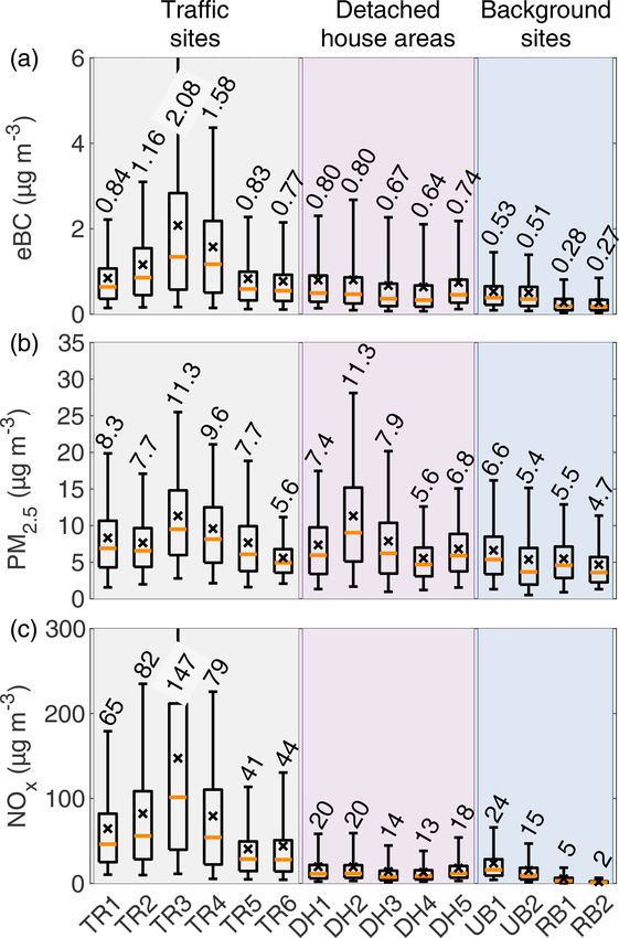
1174                                                                      K. Luoma et al.: Spatiotemporal variation and trends

lated to cardiovascular diseases, the second largest cause for      of combustion sources, which in HMA are mainly traffic and
the PM2.5 -related premature deaths were lung and respira-          residential wood combustion (Helin et al., 2018; Savolahti et
tory diseases, and a small fraction was due to lung cancer          al., 2016), affected the BC concentrations. In this study, we
(Lelieveld et al., 2015). The causes for the adverse health ef-     utilize BC data measured at various different locations in the
fects of PM are the PM-induced inflammation and toxic ma-           HMA and at one site outside the HMA. The measurements
terials which are transported in the respiratory system by the      were conducted during 2007–2018. To study how the vari-
particles.                                                          ability of BC differed from the variability of the monitored
   The WHO reported that PM emitted from combustion                 and regulated air quality parameters, we also included paral-
sources, especially from traffic, is more harmful for health        lel measurements of PM2.5 and NOx in this study.
than PM from other sources (Krzyżanowski et al., 2005).
Typical combustion sources, which are also discussed in this
study, are traffic and domestic wood burning. Traffic emits a       2     Measurements and methods
complex mixture of gaseous and fine particulate compounds
(Rönkkö and Timonen, 2019). Domestic wood burning also              2.1    The field sites
emits fine particles that include toxic compounds, such as
benzo(a)pyrene (Hellén et al., 2017). Black carbon (BC),            The HMA consists of four different cities (Helsinki, Espoo,
which is defined as black carbonaceous particulate matter,          Vantaa, and Kauniainen), and it is the most densely popu-
is a good indicator of pollution from combustion because            lated area in Finland. In 2020, the total population in the
it is a side product of incomplete combustion. Therefore,           HMA was about 1.4 million. Helsinki is the capital of Fin-
measuring BC alongside the other air quality parameters can         land, and it is located on the southern coast of the country
give additional information about the health effects of PM          (60◦ 100 N, 24◦ 560 E). The HMA is situated on the seaside
(Janssen et al., 2011). BC is not just an indicator of bad air      of the Gulf of Finland, and therefore the climate in the area
quality, but the BC particles themselves also have adverse          is a transition zone between oceanic and continental climate
health effects. BC particles, which are around the size range       and is typically defined as a humic continental climate. On
of ∼ 100 nm, can penetrate deep in the respiratory system           average, the coldest month during the measurement period
and all the way to the alveolar region where the particles can      (2009–2018) was February (−5 ◦ C), and the warmest month
be transported in the blood circulation system and further on       was July (19 ◦ C). The mean wind speed over the whole mea-
into the organs.                                                    surement period was about 4 m s−1 . For more detailed infor-
   Due to its black appearance, BC absorbs solar radiation          mation about the meteorological parameters, see Fig. S1.
and decreases the albedo of reflecting surfaces (i.e., snow            The measurements of BC concentration were conducted at
and ice sheets). BC has been estimated to be one of the great-      15 sites. We classified the stations into four categories: traf-
est warming agents in climate change (Stocker et al., 2013).        fic site (TR), detached housing area (DH), urban background
Since BC is emitted in the air as particles, its lifetime in        (UB), and regional background (RB). The locations of the
the atmosphere is relatively short (a few weeks) compared           measurement sites are presented in Fig. 1; the exact coordi-
to greenhouse gases (tens of years). Therefore, in addition to      nates and aerial photos of the stations are provided in Sect. S2
improving air quality, cutting down the BC emissions would          in the Supplement. A total of 14 of the measurements sites
have rather fast effects in the radiative forcing slowing down      were located in the HMA, and one of the RB sites was lo-
the rate of global warming. In order to reduce BC emissions,        cated circa 200 km north of the HMA in Hyytiälä. At some
there has been, for example, a suggestion of implementing           of the stations, the measurements have been repeated or con-
a BC footprint similar to the CO2 footprint (Timonen et al.,        ducted on a long-term basis, and at some of the stations, the
2019).                                                              measurements lasted only for 1 year. The measurement peri-
   Several recent studies have reported decreasing long-term        ods for each site are given in Table 1.
trends in BC concentration in different types of environments          Six traffic stations, TR1–TR6, were located close to a busy
including urban areas (e.g., Sun et al., 2020; Kutzner et al.,      street or road (Sect. S2.1). At these sites, traffic was the dom-
2018; Singh et al., 2018; Font and Fuller, 2016). In Finland,       inant source of pollution. Detailed information, such as traf-
the concentration of BC and its trends have been studied es-        fic counts (TCs), fraction of heavy-duty vehicles (HD; i.e.,
pecially in background sites (Hienola et al., 2013; Hyvärinen       trucks and buses), and the distance of the station to the clos-
et al., 2011) but not that much in urban areas. The previous        est traffic lines are presented in Table 2.
studies about BC concentrations in the Helsinki metropolitan           Detached housing stations, DH1–DH5, were located
area (HMA) were mainly from shorter campaigns (Aurela et            in residential areas that consisted of separate one-family
al., 2015; Dos Santos-Juusela et al., 2013; Helin et al., 2018;     houses, small streets, and some forests and parks (Sect. S2.2).
Järvi et al., 2008; Pakkanen et al., 2000; Pirjola et al., 2017).   The traffic rates at these areas were low; for example, the
   The objective of this study is to investigate the spatiotem-     traffic rates on the streets next to DH1 and DH5 were about
poral variability of BC in different types of environments in       2600 vehicles per day, which was significantly less than at
the HMA. Our objective is also to clarify how the proximity         the TR sites (Table 2). According to a survey study, up to

Atmos. Chem. Phys., 21, 1173–1189, 2021                                               https://doi.org/10.5194/acp-21-1173-2021
K. Luoma et al.: Spatiotemporal variation and trends 1175
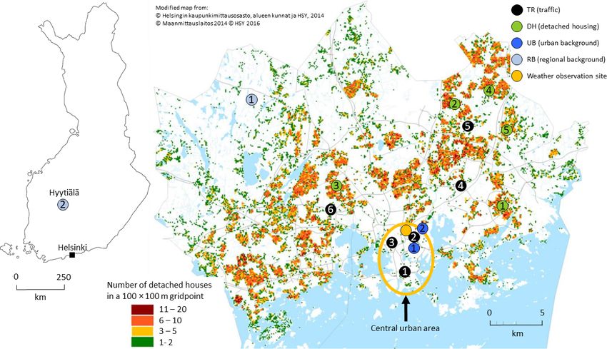
Figure 1. Location of the stations and density of the detached houses. Differently colored markers indicate different station categories. The
central urban area is marked on the map with an orange circle.
Table 1. Annual mean values of eBC concentration for each station (in units of µg m−3 ). The annual means at UB2 in 2016–2017 are
bracketed since there was less than 50 % of valid data.
Station 2007 2008 2009 2010 2011 2012 2013 2014 2015 2016 2017 2018
TR1 1.27 0.90 0.81 0.72 0.80 0.68 0.73
TR2 1.35 1.24 1.08 0.99
TR3 2.64 1.55
TR4 1.58
TR5 0.91 0.76 0.83
TR6 0.88 0.67
DH1 0.80
DH2 0.80
DH3 0.65
DH4 0.64
DH5 0.74
UB1 0.68 0.59 0.53 0.52 0.50 0.42 0.49
UB2 0.54 (0.56) (0.44) 0.50
RB1 0.26 0.29
RB2 0.31 0.38 0.33 0.39 0.33 0.48 0.19 0.24 0.19 0.20 0.16 0.19
90 % of the one-family households burned wood to warm up were located close to the central area but not in the vicinity
houses and/or saunas, but less than 2 % of the households of busy roads (Sect. S2.3). UB2 is also known as SMEAR III
used wood combustion as the main heating source (HSY, (Station for Measuring Ecosystem–Atmosphere Relations;
2016, in Finnish only; Hellén et al., 2017). Järvi et al., 2009). Regional background stations RB1 and
Background sites were categorized as urban and regional RB2 were located in rural areas about 20 and 200 km away
background sites. Urban background stations, UB1 and UB2, from Helsinki, respectively (Sect. S2.3). RB sites represented
https://doi.org/10.5194/acp-21-1173-2021 Atmos. Chem. Phys., 21, 1173–1189, 20211176 K. Luoma et al.: Spatiotemporal variation and trends
Table 2. Traffic counts for working days at the nearest streets to the TR sites. Traffic counts and the fraction of the heavy-duty vehicles are
from the yearly Helsinki traffic reports. The streets and roads mentioned here are marked in Fig. S3.
Station Street name Traffic count Heavy-duty Distance to street Reference
(vehicles/weekday) vehicles (%) edge (m) year
TR1 Mannerheimintie 15 800 11 3 2017
Kaivokatu 20 100 8 40 2017
TR2 Mäkelänkatu 28 100 11 0.5 2017
TR3 Mannerheimintie 44 400 14 0.5 2010
Reijolankatu 19 400 – 25 2010
TR4 Kehä I 69 200 8 5 2012
Tattariharjuntie 13 700 13 120 2012
TR5 Tikkurilantie 9500 – 7 2016
TR6 Turuntie 29 300 4 20 2017
Lintuvaarantie 15 400 5 30 2017
Kehä I 68 900 4 250 2017
the concentration levels outside the urban area without local was air warmed up to room temperature, which decreased the
pollution sources. RB2 is also part of the SMEAR network RH when the outdoor temperature was lower than the indoor
and is better known as SMEAR II (Hari and Kulmala, 2005). temperature (i.e., the sample air was dried passively during
The Helsinki Region Environmental Services Authority the cold period; however, in summer, when the temperature
(HSY), which is the authority monitoring the air quality in difference was smaller, the RH did not necessarily decrease).
the HMA, arranged the measurements at 13 of the sites. The MAAP determines the absorption coefficient of
The Institute for Atmospheric and Earth System Research aerosol particles by collecting the particles on a filter medium
(INAR) arranged the measurements at RB2, and the Finnish and by measuring the intensity of light penetrating the fil-
Meteorological Institute (FMI), together with INAR, con- ter and the intensity of light that is scattered from the fil-
ducted the measurements at UB2. ter at two different angles (Petzold and Schönlinner, 2004).
The absorption coefficient is determined from these measure-
2.2 Measurements of equivalent black carbon ments by using a radiative transfer scheme. The eBC concen-
tration is obtained from the absorption coefficient by using a
All BC measurements were conducted optically, meaning mass absorption cross-section (MAC) value of 6.60 m2 g−1
that the BC concentration was derived from the light absorp- (Petzold and Schönlinner, 2004). The MAAP operates only
tion of the particles, and hence we refer to the measured BC at one wavelength, which is 637 nm.
as equivalent black carbon (eBC; Petzold et al., 2013). At The aethalometer measures the eBC concentration at seven
11 of the stations, the measurements of eBC were conducted wavelengths (370, 470, 520, 590, 660, 880, and 950 nm).
by using only a multi-angle absorption photometer (MAAP; Here we chose to use the 880 nm channel since it is the rec-
Thermo Fisher Scientific, model 5012), and at three of the ommended and most commonly used wavelength to report
stations (DH4, DH5, and RB2), all or at least part of the mea- the eBC measured by an aethalometer. Similar to the MAAP,
surements were conducted by using an aethalometer (Magee the aethalometer collects the sample aerosol particles on the
Scientific, models AE31 and AE33). The instruments used at filter material, but unlike the MAAP, the aethalometer only
the different sites are listed in Table S1. measures the attenuation of light through the filter. There-
At all of the stations, the head of the sampling line was fore, the aethalometer is prone to error caused by the increas-
located 4 m above the ground. The concentration of eBC was ing filter loading. In the newer model, AE33, this is auto-
measured for particles smaller than 1 µm (PM1 ). However, at matically taken into account in real time as the instrument
DH1, the eBC concentration was measured for PM2.5 for the applies the so-called “dual-spot correction” to the data (Dri-
first half of the year, but since most of the BC particles are novec et al., 2015). For AE33, the recommended MAC value
smaller than 1 µm in diameter (Vallius et al., 2000), the cut- of 7.77 m2 g−1 at 880 nm was used in this study (Drinovec et
off size should not have caused a big difference in the results. al., 2015). For the older model, AE31, a correction algorithm
Sample air was dried with an external dryer or by warming needs to be applied by the user (e.g., Collaud Coen et al.,
up the sample to 40 ◦ C at most of the stations, but at TR1, 2010). AE31 determines the BC concentration from the so-
UB2, DH5, and DH4 (only the first half of the year), the sam-
ple air was not dried. Even if there was no drier, the sample
Atmos. Chem. Phys., 21, 1173–1189, 2021 https://doi.org/10.5194/acp-21-1173-2021K. Luoma et al.: Spatiotemporal variation and trends 1177
called attenuation coefficient, and it uses a mass attenuation 2.4 Meteorological measurements
cross-section value of 16.62 m2 g−1 at 880 nm.
At DH4, a model AE33 aethalometer was used for the The meteorological station measuring wind direction (WD),
first half of the measurement period (1 January 2017–5 May wind speed (WS), temperature (T ), pressure (p), relative
2017), and at DH5, the whole data set was measured with an humidity (RH), and precipitation was located on a rooftop
AE33. At these two stations, HSY corrected the eBC con- (78 m a.s.l.) close to central Helsinki (Fig. 1). In this study,
centration by multiplying the concentration by 0.75 accord- we used the measurements of meteorological parameters
ing to a comparison with MAAP. At RB2, an older model, conducted at the rooftop station to represent the meteorolog-
AE31, was used. The AE31 was first corrected for the fil- ical conditions of all stations located in the HMA. We also
ter loading error by using the correction algorithm suggested included data of the mixing height (MH) for southern Fin-
by Virkkula et al. (2007). After the filter loading correction, land. The MH was calculated by MPP-FMI, a meteorologi-
a comparison with MAAP showed that the AE31 data had cal preprocessing model developed by the FMI (Karppinen
to be multiplied by 1.08 to acquire similar concentrations et al., 2000).
(Sect. S3).
2.5 Data processing
2.3 Measurements of NOx and PM2.5
The data quality was assured by the data producer, and in-
NO2 and the mass of particles smaller than 2.5 µm (PM2.5 ) valid data were omitted from further analysis. The concen-
are regulated pollutants based on the air quality directive trations were converted to ambient outdoor temperature and
2008/50/EC, and therefore they are always measured at the to normal atmospheric pressure (1013.25 hPa). In this study,
air quality stations. In this study, we used NOx (NO + NO2 ) we used 1 h averages for all the variables (the only excep-
data instead of the regulated NO2 since NOx describes better tion is the PM2.5 data at RB2). The hourly mean values were
the primary traffic emissions. Even though there was much calculated if the hour had at least 75 % valid data. The hour
more NOx and PM2.5 data available compared to eBC data, of day always refers to the local time (note that winter and
we used only NOx and PM2.5 data that were measured paral- summer times are used in Finland), and the time stamp of
lel to eBC in order to make the comparison and trend analysis the measurements is reported in the middle of the averaging
systematic. period.
The PM2.5 concentration was measured with various dif-
ferent instruments, which are listed for each station in Ta- 2.6 Trend analysis
ble S1. The instruments were based on four different meth-
ods: (1) attenuation of β radiation (Thermo model FH 62 We used the seasonal Mann–Kendall test and Sen’s slope es-
I-R), (2) tapered element oscillating microbalance (TEOM; timator (Gilbert, 1987) in determining the statistical signif-
Thermo different models), (3) optical detection (Grimm icance and the slopes of the long-term trends. The Mann–
180), and (4) collecting the particles in a cascade impactor Kendall test and Sen’s slope estimator are non-parametric
and manually weighing the collected particles. The instru- statistical methods which allow missing data points. The
ments, which apply methods 1–3, measure the concentration method determines the trends for each season (here we used
continuously. At RB2, where the PM2.5 concentration was months) separately and tests if the trends for different seasons
measured by collecting the particles in a cascade impactor are homogeneous. We used monthly median values in the
and weighing the collected particles about three times a week trend analysis, and we required at least 14 d of valid data for
so the time interval of these measurements varied from 2 to 3 each month; otherwise the month was not taken into account
days. To compare the PM2.5 measurements to BC concen- in the trend analysis. A similar analysis has been used in var-
tration at RB2, the PM2.5 concentration was interpolated to ious trend studies (e.g., Collaud Coen et al., 2007, 2013; Li
match the timestamps of the eBC measurements. et al., 2014; Zhao et al., 2017).
NOx mass concentration [NOx ] was derived from the mea-
surements of NO and NO2 so that
3 Results and discussion
[NOx ] = 1.533 · [NO] + [NO2 ] . (1)
3.1 Spatial variation
The mass concentration of NO and NO2 was measured
by instruments which are based on the chemiluminescence The statistics of eBC, PM2.5 , and NOx concentrations from
method. The instruments used at each station are listed in each site are presented in Fig. 2. The figure includes all the
Table S1. data, and the statistics were determined by using the 1 h mean
values. Figure 2 shows that the arithmetic mean values dif-
fered from the median values, which means that the data of
the air pollutants were not normally distributed at any station
and that the data were skewed to the right (i.e., small concen-
https://doi.org/10.5194/acp-21-1173-2021 Atmos. Chem. Phys., 21, 1173–1189, 20211178 K. Luoma et al.: Spatiotemporal variation and trends
vehicles (Clougherty et al., 2013; Weichenthal et al., 2014).
The surrounding buildings, vegetation, and the wind condi-
tions affect the dilution and therefore the BC concentrations
as well (Abhijith et al., 2017; Brantley et al., 2014; Pirjola
et al., 2012). Also, nearby intersections may affect the BC
concentrations if they induce traffic buildups; BC emissions
from vehicles that accelerate are higher than the emissions
from a steadily moving vehicle (Imhof et al., 2005).
The abovementioned factors are probably the reason for
the relatively big differences between the different TR sta-
tions and explain, for example, why the eBC concentration
at TR3 was notably higher than at the other TR sites. TR3
was located in a street canyon right next to a very busy traf-
fic line. According to Table 2, the traffic count on the closest
street next to TR3 was around 44 400 vehicles per weekday
and the fraction of heavy-duty vehicles was 14 %. The traffic
count and fraction of heavy-duty vehicles was higher than,
for example, on the street next to TR1 or on the street next
to TR2. The area around TR3 also consisted of a few busy
intersections, and the location in a street canyon probably in-
creased the eBC concentrations even further.
The effects of total traffic count and traffic count of heavy-
duty vehicles (HD) on the eBC concentration were studied
Figure 2. Statistics of the (a) eBC, (b) PM2.5 , and (c) NOx con-
in more detail in the Supplement (Fig. S9), in which the an-
centrations at each station. The boxplots are presented for 1 h mean
values. The orange line in the middle of each box represents the me- nual mean eBC concentrations were compared against the
dian, the edges of the boxes represent the 25th and 75th percentiles, estimated weekday traffic counts of all vehicles and of HD
and the whiskers represent the 5th and 95th percentiles. The black vehicles on the nearest street or road. The annual means of
cross is the arithmetic mean, and its numerical value is reported eBC concentration correlated better with the number of HD
above each box. The background color represents the station type: vehicles passing the station (R = 0.82) than with the total
gray for traffic sites (TRs), purple for the detached housing sites traffic count (R = 0.71). In general, the number of HD ve-
(DH), and blue for the background sites (UB for urban and RB for hicles passing TR1, TR5, and TR6 per day was low com-
regional background). The 75th percentiles of the eBC and NOx pared to TR2, TR3, and TR4, and this was also seen in the
concentration at TR3, which are not visible at the figure, were 6.7 mean concentration of eBC, which was the highest for the
and 440 µg m−3 , respectively.
TR2–TR4. This result was expected since the BC emissions
from HD vehicles are higher compared to light-duty vehicles
(Imhof et al., 2005).
trations occurred more often, and therefore the median values The distance from the stations to the edge of the nearest
were smaller than the means). street varied, which has an effect on the measured eBC con-
As expected, the highest mean eBC concentrations were centration (Massoli et al., 2012; Zhu et al., 2002). A study
observed at the TR sites where the mean eBC concentration by Enroth et al. (2016) estimated that eBC concentration de-
varied from 0.77 to 2.08 µg m−3 (at TR6 and TR3, respec- creased by 50 % at 33 m distance from the road. TR2 and
tively). At the DH sites, the mean eBC concentration varied TR3, where we observed rather high concentrations, were
from 0.64 to 0.80 µg m−3 , which were rather similar mean located right next to the street (in a 0.5 m distance), whereas
values as observed at TR1, TR5, and TR6 (0.84, 0.83, and the other stations had a longer distance to the nearest street
0.77 µg m−3 , respectively). At the UB sites, the mean eBC (3–20 m). Previous studies have also shown that tall trees in
concentrations were around 0.52 µg m−3 , which was clearly street canyons may deteriorate the air quality by preventing
lower than at the TR and DH sites. The lowest mean eBC dispersion (Abhijith et al., 2017), and this may also have af-
concentrations, which were around 0.27 µg m−3 , were ob- fected the higher measured concentrations at TR2 and TR3.
served at the RB sites that had no local BC sources in the On Mäkelänkatu street, which is next to TR2, there are two
vicinity. lines of trees framing the tram lines in the middle of the
Previous studies have shown that in addition to the traf- street (Fig. S3b), and on Mannerheimintie street, which is
fic count, the BC concentration near traffic lines depends on next to TR3, there are trees planted between the traffic lines
various factors: the distance to the traffic lines (Enroth et and pavements (Fig. S3c).
al., 2016; Massoli et al., 2012; Zhu et al., 2002), the speed Compared to the HMA, higher concentrations of eBC
limit (Lefebvre et al., 2011), and the fraction of heavy-duty have been reported at other urban areas in Europe. For ex-
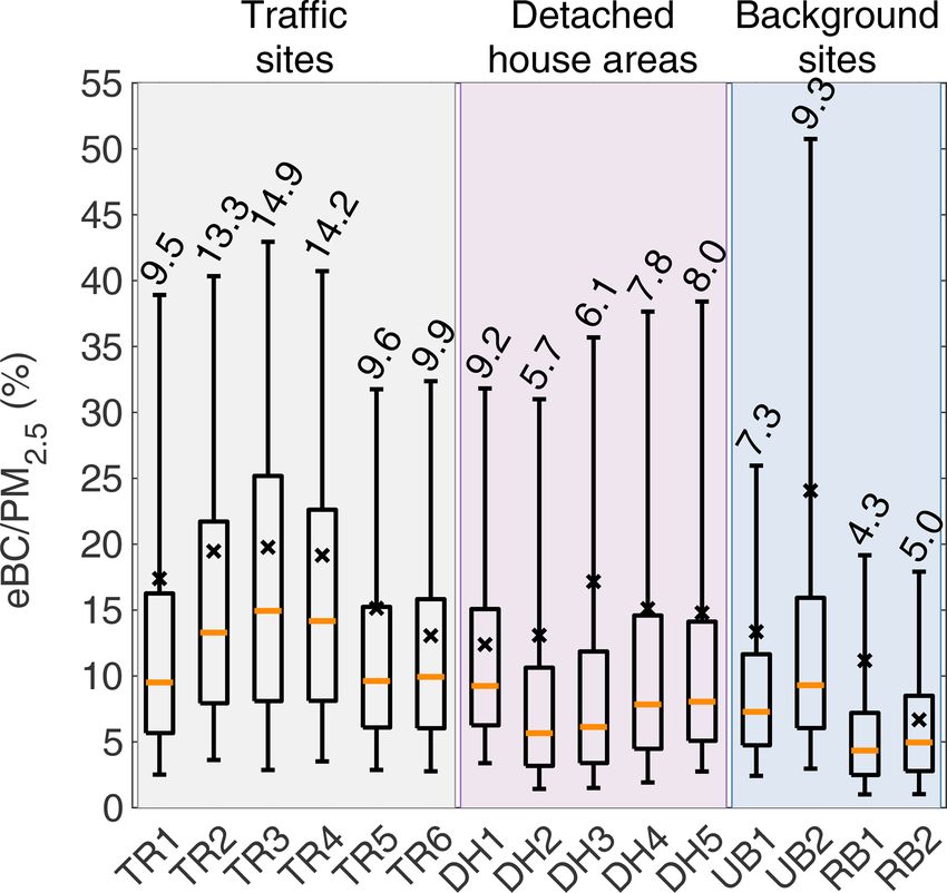
Atmos. Chem. Phys., 21, 1173–1189, 2021 https://doi.org/10.5194/acp-21-1173-2021K. Luoma et al.: Spatiotemporal variation and trends 1179 ample, Sun et al. (2019) reported median values of 2.0, 0.9, and 0.4 µg m−3 at several German TR, UB, and RB sites, respectively, measured during 2009–2018. Singh et al. (2018) reported on average eBC concentrations of 1.83 and 1.34 µg m−3 measured at several urban center and UB sites in the United Kingdom during 2009–2011. Krecl et al. (2017) observed a mean eBC concentration of 2.1 µg m−3 at a street canyon site in Stockholm during weekdays in spring 2013. Becerril-Valle et al. (2017) reported mean eBC values of 3.7 µg m−3 at a TR site and 2.33 µg m−3 at a UB site measured in Madrid in 2015. The BC concentrations re- ported by other studies at different environments are higher than the eBC concentrations measured at corresponding en- vironments in the HMA. Already the concentrations at the RB sites are lower than those measured at other European Figure 3. Statistics of eBC/PM2.5 fraction at each station. The ex- sites. Generally, the air quality in the HMA and in southern planation for the markers is the same as in Fig. 2, except here the Finland was good. Finland is isolated from the more pop- values reported above each box are the median values. ulated continental Europe by the Baltic Sea, and therefore long-range pollution from the more polluted continental area affects southern Finland less. Due to its coastal location, the HMA is affected by the sea breeze, and the air is therefore lower as it was for eBC and NOx . These results show that well diluted. Compared to other European metropolitan ar- PM2.5 did not depend on local primary pollution sources as eas, the HMA is small and the area is not as densely popu- much as eBC or NOx did. PM2.5 includes all different kinds lated as many other European capital areas. of aerosol particles, especially secondary aerosol, which may In addition to eBC, we also studied the variations in PM2.5 be anthropogenic or biogenic in origin. In this size range, and NOx , presented in Fig. 2b and c, respectively. The spa- non-anthropogenic particles (e.g., secondary particles of bio- tial variation in NOx was partly similar to that of eBC; the genic origin; Dal Maso et al., 2005) are also contributing. The highest concentrations were measured at the TR sites and the differences in the sources of eBC and PM2.5 concentrations lowest at the RB sites. At the TR sites, the mean concentra- were also seen in the correlation between these two variables; tions varied between 44 and 147 µg m−3 (at TR5 and TR3, re- the R between these two variables at different stations were spectively), and the variation between the stations was rather notably lower (0.36 ≤ R ≤ 0.67) than the R between eBC similar to the variation in eBC. Like BC, NOx is highly de- and NOx concentrations (Fig. S7b). pendent on the traffic-related parameters, such as the traf- The fraction of eBC in the PM2.5 is shown in Fig. 3. The fic count, the fraction of heavy traffic, the speed limit, etc., eBC was measured mostly in PM1 , but since most of the BC which explains the similar variation observed. For the RB particles are smaller than 1 µm in diameter, the difference be- sites, however, the mean NOx (around 2 µg m−3 ) was rela- tween the cut-off diameters should not have a big effect on tively low compared to eBC at RB sites. Another difference the results (e.g., Enroth et al., 2016). The higher eBC/PM2.5 to eBC was that the NOx concentration at the DH sites was ratio indicates that there was a larger fraction of PM sources relatively lower, which was expected since the NOx emis- related to combustion. The highest median eBC/PM2.5 ratio sions from residential wood combustion are low. The corre- was observed at the TR sites where the fraction of eBC varied lations between eBC and NOx concentrations at each station from 10 % to 15 %. The second highest median ratios were are presented in Fig. S8a. As the likeness in the spatial vari- observed at the DH sites and at UB1 where the ratios varied ability already suggested, the eBC and NOx had rather sim- from 5 % to 9 %. At the RB sites, the median fractions were ilar sources, and therefore they were expected to correlate. the smallest: about 5 %. The correlation coefficient (R) between these variables was The results of the spatial variation showed that eBC con- the highest at the TR stations (0.80 ≤ R ≤ 0.90) and lower at centration and eBC/PM2.5 ratio depended greatly on the dis- the DH stations (0.63 ≤ R ≤ 0.73). At the background sites, tance to the pollution sources, which were, in this case, traffic the correlation coefficient varied more (0.55 ≤ R ≤ 0.83). and wood combustion. The NOx was very dependent on the For PM2.5 , there were not as clear patterns between dif- distance to the traffic sources only since NOx concentration ferent station categories as there were for eBC and NOx . was not significantly affected by residential wood combus- At the TR sites, the mean PM2.5 concentration varied from tion. Since the PM2.5 has various sources and generally high 5.6 to 11.3 µg m−3 (at TR6 and TR3, respectively), and at background levels, it was the component least dependent on the DH sites, the variation was rather similar: from 5.6 to the contribution of the local sources. 11.3 µg m−3 (at DH4 and DH2, respectively). The mean con- Figures 2 and 3 include all the data that were collected centration of PM2.5 at the background sites was not as clearly from 2009 to 2018, whereby the sizes of the data sets at each https://doi.org/10.5194/acp-21-1173-2021 Atmos. Chem. Phys., 21, 1173–1189, 2021
1180                                                                  K. Luoma et al.: Spatiotemporal variation and trends

station differed. Therefore, the year-to-year variation caused
by the meteorological conditions and changes in the emission
rates might have affected the results of spatial variability es-
pecially at sites that contained only 1 year of data (all DH
sites and TR4).
   At DH4, DH5, and RB2, at least part of the measurements
were conducted by an aethalometer. The aethalometer mea-
sured the eBC at 880 nm, which is a longer wavelength than
MAAP operated at (637 nm). This could have caused some
difference in the measured eBC concentration in the pres-
ence of so-called brown carbon. Brown carbon is organic
material, which absorbs light especially at short wavelengths
(Andreae and Gelencsér, 2006). However, since the organic
carbon absorbs light mainly at wavelengths below 600 nm
(Kirchstetter et al., 2004), the difference between the MAAP
and aethalometer wavelengths should not cause a notable ef-
fect on the observed eBC concentration.
   As mentioned in Sect. 2.2, we applied constant mass ab-
sorption cross-section (MAC) values to convert the optically
measured absorption data to eBC concentration. However,
the MAC may vary depending on the chemical composition,
shape, and the mixing state of the PM. The MAC increases
for aged BC particles as the BC particles get coated with a
scattering or slightly absorbing coating which acts as a lens      Figure 4. Time series and trends in eBC concentration at TR1, TR2,
increasing the absorption of the BC core (Lack and Cappa,          UB1, and RB2. The solid black line represents the monthly me-
2010; Yuan et al., 2020). At TR sites, the freshly emitted BC      dians, the dashed lines represent the 10th and 90th monthly per-
particles from local traffic probably have no coating on the       centiles, and the orange line is the fitted long-term trend.
particles, but at the remote sites, however, particles are car-
ried over longer distances, and the observed BC at these sites
is more aged and likely more coated. Therefore, it is prob-        there were 4 years of measurements at UB2, the station was
able that the real MAC at the background sites was higher          omitted from the trend analysis since the data availability
compared to TR sites. If the differences in the MAC values         at UB2 in 2016–2017 was not good enough. The seasonal
were taken into account, it could possibly increase the dif-       Mann–Kendall test was applied to monthly medians values
ference between the traffic and background sites. The source       which are presented in Fig. 4 for the eBC concentration at
of the BC may also have an effect on the MAC, but, for ex-         TR1, TR2, UB1, and RB2. We could not apply the trend anal-
ample, Yuan et al. (2020) and Zotter et al. (2017) did not         ysis to any of the DH stations since none of the DH stations
observe a notable difference between the MAC for particles         had more than 1 year of eBC measurements.
originating from traffic or wood combustion. In addition to           A statistically significant (p value < 0.05) decreasing
spatial variation, the MAC can also vary temporally, which         trend was observed for all of the stations included in the trend
could affect the observed seasonal and diurnal variations and      analysis (TR1, TR2, UB1, and RB2) as shown in Fig. 4 and
trends (presented in Sect. 3.2) as well. However, determin-        in Table 3. The smallest absolute decrease was observed at
ing the variations in MAC would require extensive long-term        the background stations UB1 and RB2, for which the slopes
measurements of the chemical composition of the BC parti-          of the trends were −0.02 and −0.01 µg m−3 yr−1 , respec-
cles in different environments, and therefore further analysis     tively. At TR1, the concentration decreased more rapidly
of the effect of MAC is omitted here.                              by −0.04 µg m−3 yr−1 , and at TR2, the decrease was even
                                                                   greater: −0.09 µg m−3 yr−1 . In addition to the absolute trend,
3.2     Temporal variation                                         we also determined the relative trends by dividing the ab-
                                                                   solute slope of the trend by the overall median concen-
3.2.1    Long-term trends                                          tration. At TR1, UB1, and RB2, the relative trends were
                                                                   rather similar: −6.4 % yr−1 , −5.9 % yr−1 , and −6.3 % yr−1 ,
Table 1 already showed that the annual eBC mean values             respectively. At TR2, the decrease was relatively steeper:
had seemingly decreased. To see if the decreasing eBC trend        −10.4 % yr−1 .
had a statistical significance, we applied the seasonal Mann–         One possible cause for the decreased pollution concen-
Kendall test (see Sect. 2.4.1) to the data sets that were at       trations could have been the changes in the meteorological
least 4 years long (TR1, TR2, RB2, and UB1). Even though           parameters that affect the dilution. Teinilä et al. (2019) re-

Atmos. Chem. Phys., 21, 1173–1189, 2021                                              https://doi.org/10.5194/acp-21-1173-2021
K. Luoma et al.: Spatiotemporal variation and trends 1181
Table 3. Results of the trend analysis of the eBC, PM2.5 , and NOx concentrations. The values without brackets are the absolute trends (in
units of µg m−3 yr−1 ), the values in the square brackets are the 5th and 95th uncertainty limits of the trend (in units of µg m−3 yr−1 ), and
the bracketed values are the relative trends (in units of % yr−1 ). The values for PM2.5 at TR2 are italicized since they were statistically not
significant (p value = 0.05).
Station eBC (µg m−3 yr−1 ) PM2.5 (µg m−3 yr−1 ) NOx (µg m−3 yr−1 ) Measurement years
TR1 −0.04 −0.24 −3.11 2011,
[−0.06; −0.02] [−0.38; −0.01] [−4.18; −1.87] 2013–2018
(−6.5 % yr−1 ) (−3.7 % yr−1 ) (−7.1 % yr−1 )
TR2 −0.09 −0.46 −11.00 2015–2018
[−0.11; −0.05] [−0.71; 0.02] [−12.47; −8.70]
(−10.6 % yr−1 ) (−7.1 % yr−1 ) (−19.7 % yr−1 )
UB1 −0.02 −0.20 −0.80 2012–2018
[−0.03; -0.01] [−0.34; −0.05] [−1.08; −0.50]
(−5.7 % yr−1 ) (−3.9 % yr−1 ) (−5.0 % yr−1 )
RB2 −0.01 −0.09 −0.05 2006–2018
[−0.01; −0.01] [−0.18; −0.03] [−0.09; −0.03]
(−6.3 % yr−1 ) (−2.6 % yr−1 ) (−4.9 % yr−1 )
ported that in the HMA, the two most important meteorolog- between the years 2010 and 2015 (Table 1), the trend at TR3
ical parameters that affected the PM1 concentrations were was also studied, which is presented in Sect. S5. The analysis
wind speed (WS) and temperature (T ); Järvi et al. (2008) showed that the concentrations of eBC, NOx , and PM2.5 de-
observed that of the meteorological parameters, the WS and creased about −12.2 % yr−1 , −8.2 % yr−1 , and −5.6 % yr−1 ,
mixing height (MH) affected the BC concentration the most. respectively. Also at TR3, the PM2.5 concentration decreased
The highest concentrations were observed at low WS and relatively the slowest.
MH conditions and when the T was either very high in sum- Compared to PM2.5 , the concentrations of eBC and NOx
mer or very low in winter, which indicates stable and stag- were more sensitive to the changes in the traffic since they
nant meteorological conditions. Also, a temperature decrease are more dependent on the local sources than PM2.5 , as dis-
during colder periods could increase the emissions from res- cussed in Sect. 3.1. Therefore, the greater decrease in eBC
idential wood combustion. Therefore, in addition to BC, we and NOx concentrations indicated that especially the emis-
ran the trend analysis for the time series of WS, T , and MH sions from traffic had decreased. Since PM2.5 is not as sen-
(time series in Fig. S1). However, we did not observe statis- sitive to changes in primary traffic-related emissions, it ex-
tically significant trends for any of these parameters. We also plains why the slope of the trend for PM2.5 was relatively
studied the trends for the different seasons separately to see, smaller than that of eBC and NOx . In other words, since the
for example, if the temperatures had increased in the summer pollutant emissions from traffic sources have generally de-
months or decreased in winter months, but this analysis did creased, it clearly affected the trends in eBC and NOx which
not yield statistically significant trends either. Therefore, it is are originating from local traffic sources but to a lesser ex-
likely that the decreasing trends in the eBC concentration can tent the trend in PM2.5 . Even though the decrease in local
not be explained by the meteorological factors. traffic emissions was the probable explanation for the de-
To see how the decrease in eBC concentrations compared creasing trends especially at the TR and UB sites, changes in
to the trends in other air pollutants, we conducted the trend the long-range transported pollution likely affected the trends
analysis also for the PM2.5 and NOx data. The resulting as well. Statistically significant trends were observed also at
trends are also presented in Table 3. The only parameter RB2, indicating that the long-range transported pollution and
for which we did not observe a statistically significant de- the emissions in the regional area had also decreased.
creasing trend was PM2.5 at TR2 (p value = 0.05). The rela- For eBC and NOx , it is difficult to say which one of the
tive trends varied from station to station, but a common trait pollutants decreased at a faster rate. Their relative decreases
was that the concentrations of eBC and NOx decreased rel- were rather similar at TR1, UB1, and RB2. At TR2, there
atively faster than the concentration of PM2.5 . The trends was a large difference and NOx seemed to decrease at dou-
in NOx concentration varied from −19.7 % yr−1 (TR3) to ble the rate compared to eBC, which could be caused, for
−4.9 % yr−1 (RB2), and the trends in PM2.5 concentration example, by the fast renewal of the city bus fleet. Accord-
varied from −3.9 % yr−1 (UB1) to −2.6 % yr−1 (RB2). Since ing to the Helsinki Regional Transport Authority (HSL), in
there was a notable decrease in the eBC concentration at TR3 2015, about 17 % of the HSL buses were Euro VI, and in
https://doi.org/10.5194/acp-21-1173-2021 Atmos. Chem. Phys., 21, 1173–1189, 20211182 K. Luoma et al.: Spatiotemporal variation and trends
by a disturbance of the air conditioning. In principle, the di-
urnal trends indicated that the primary emissions from traf-
fic have decreased most prominently, i.e., changes in traffic
regulations and technological advancements have especially
decreased the eBC and NOx emissions.
According to the report about traffic in Helsinki, the traf-
fic volume in Helsinki increased a bit, by 0.4 % yr−1 , dur-
ing the period 2006–2016 (Helsinki, 2017, in Finnish only).
However, in general, the number of vehicles entering and
exiting the city center (represented by TR1) decreased by
1.5 % yr−1 , and the number of vehicles entering and exiting
the central urban area (represented by TR2, TR3, and UB1)
decreased by 0.8 % yr−1 during the same period, which ob-
viously decreases the emissions from traffic. The decreases
in traffic rates were especially observed in the northwest-
ern part of the central urban area (e.g., Fig. S10c), which
probably affected the trends observed at TR3. However, on
Mäkelänkatu, which is the main street next to TR2 where
decreasing trends were also observed, there was no clear de-
crease in the traffic rate (Fig. S10f).
Since the traffic rates did not decrease at all of the stations,
it can be concluded that the decreasing trends were due to the
renewal of vehicle and bus fleet, as well as cleaner renewable
fuels which have been shown to decrease both BC and NOx
Figure 5. Annual trends for the hourly data. Here, only data from emissions (Järvinen et al., 2019; Pirjola et al., 2019; Timonen
weekdays were used. None of the pollutants had a positive trend for et al., 2017). The exhaust particle number of diesel and gaso-
any time of the day. line vehicles has been regulated efficiently in order to reduce
the traffic emissions. The regulations have enforced the use
of diesel particulate filters (DPFs) in new diesel passenger
2018, the fraction had increased to about 50 %. A study by cars and heavy-duty diesel vehicles, reducing their BC and
Järvinen et al. (2019) showed that moving to Euro VI buses PM emissions even more than 90 % and up to 99 % when
from enhanced environmentally friendly vehicles (EEVs) ef- compared to the diesel vehicles without a DPF (Bergmann et
ficiently decreases the NOx emissions. However, at TR2, the al., 2009; Preble et al., 2015). Also, the increased use of bio-
short time series cause uncertainty in the trends, and, for ex- fuels and gas as vehicle fuels increased the share of electric
ample, the year-to-year variability caused by the meteorolog- vehicles, and improvements in fuel economy in internal com-
ical conditions could cause the apparent decrease in pollutant bustion engines affected the observed trends. For example,
concentrations. the increase in fuel injection pressure in diesel combustion
The trends at TR1 and UB1 were investigated in more de- can improve the fuel economy of engines and simultaneously
tail since these stations had the longest time series and they decrease the BC emissions of engines (Lähde et al., 2011).
were located closer to local sources in the HMA. To see Decreases in the eBC concentration (or absorption co-
if the traffic-related emissions affected the trends, the trend efficient) have also been observed in the Finnish arctic
analysis was conducted separately for each hour so that the (Dutkiewicz et al., 2014; Lihavainen et al., 2015). In gen-
monthly median was determined for each hour of the day. eral, declining trends in atmospheric aerosol particle number
Only the data from weekdays were included in the analysis. concentration and particulate material have been observed in
This trend analysis revealed that there were clear decreases various different types of environments in Europe (Asmi et
in the eBC and NOx concentrations around the morning rush al., 2013). Similar results for the trend in eBC concentration
hour, as shown in Fig. 5a and c. The trend in the eBC con- have been reported in several cities and countries in Europe.
centration had a distinctive diurnal cycle in general so that In Stockholm, Sweden, Krecl et al. (2017) reported about a
the decrease was more prominent during morning and day, 60 % reduction in eBC concentration in a busy street canyon
and actually there was no statistically significant trend dur- between the years 2006 and 2013 (i.e., −7.5 % yr−1 ). Singh
ing nighttime (22:00–03:00 EET). A similar diurnal pattern et al. (2018) observed a statistically significant decreasing
was observed for the PM2.5 as well; however, the pattern was trend in eBC concentration at five measurements stations
not as well defined as for the eBC. At TR1, the PM2.5 data which operated during 2009–2016 and were located in dif-
between 08:00 and 09:00 and 21:00 and 22:00 were not in- ferent types of environments in the United Kingdom. The
cluded in the trend analysis due to technical issues caused trends varied from −0.09 µg m−3 yr−1 (−4.7 % yr−1 ) at an
Atmos. Chem. Phys., 21, 1173–1189, 2021 https://doi.org/10.5194/acp-21-1173-2021K. Luoma et al.: Spatiotemporal variation and trends 1183
UB site to −0.80 µg m−3 yr−1 (−8.0 % yr−1 ) at a TR sta-
tion. A trend study based only in London reported on av-
erage a −0.59 µg m−3 yr−1 (−11 % yr−1 ) decrease in eBC
concentration at three TR sites for the period 2010–2014
(Font and Fuller, 2016). Kutzner et al. (2018) observed sta-
tistically significant decreasing BC (both eBC and elemental
carbon) trends for the period of 2005–2014 at several sites
in Germany. The trends at TR sites varied from −0.31 to
−0.15 µg m−3 yr−1 , and the trends at UB sites varied from
−0.03 to −0.02 µg m−3 yr−1 . Also, a more recent study by
Sun et al. (2020) reported decreasing relative trends in eBC
in Germany for the period of 2009–2018: from −0.19 to
−0.08 µg m−3 yr−1 (−11.3 to −5.0 % yr−1 ), from −0.08 to
−0.03 µg m−3 yr−1 (−8.1 % yr−1 to −2.3 % yr−1 ), and from
−0.03 to 0.00 µg m−3 yr−1 (−7.8 % yr−1 to −3.2 % yr−1 ) at
TR, UB, and RB sites, respectively.
These studies reported higher absolute trends compared to
the absolute trends observed in our study, which is probably
due to lower eBC concentrations in southern Finland. How-
ever, the relative trends were rather similar. Similar to this
study, other studies also observed steeper absolute trends at
TR and UB sites than at RB sites. Sun et al. (2020) observed
similar diurnal eBC trends at TR and UB sites as we did in
that the decreasing trends were the highest during the morn-
ing rush hour. In addition to eBC, Krecl et al. (2017) also
studied the trend in NOx , and Font and Fuller (2016) stud-
ied the trend in PM2.5 . Contradictory to our study, Krecl et
al. (2017) did not observe a decreasing trend in NOx , and Figure 6. Diurnal variation in eBC for different station categories:
Font and Fuller (2016) reported decreasing trends in PM2.5 (a) traffic sites that were not influenced by wood burning (TR1–
4), (b) traffic sites that were influenced by wood burning (TR5–6),
concentration which were relatively similar to the trends in
(c) detached housing sites (DH1–5), (d) urban background (UB1),
eBC concentration.
and (e) regional background (RB1). The diurnal variation is deter-
The abovementioned studies, which were conducted in ur- mined separately for the cold (from November to March) and warm
ban environments, suggested that the dominant reason for the (from May to September) periods.
decreased BC concentrations were traffic regulations. Krecl
et al. (2017) drew a connection between the decreasing eBC
concentration and the renewal of the vehicle fleet. Sun et ent station categories to study the variation more generally.
al. (2020), Singh et al. (2018), and Kutzner et al. (2018) pro- The figures were plotted by calculating the mean concentra-
posed that the reductions in eBC were linked to the local and tion each hour of each day of the week for the cold and the
national air quality policies. Font and Fuller (2016) suspected warm seasons separately. All the available data were taken
that the eBC concentration decreased due to effective filters into account when the diurnal variation from different sta-
in diesel vehicles. tions were averaged together.
The mean seasonal, weekly, and diurnal variations in eBC
3.2.2 Seasonal, weekly, and diurnal variation in BC for different station categories are presented in Fig. 6. At
TR1, TR2, TR3, and TR4 (i.e., TR1–4), the seasonal and di-
The diurnal variation in eBC was investigated separately urnal variation was different from TR5 and TR6 (i.e., TR5–
for the cold and the warm seasons. According to Fig. S1, 6), and therefore the mean diurnal variations for these sets of
the coldest 5 months typically extended from November to stations were plotted separately in Fig. 6a–c, which present
March and the warmest 5 months from May to September. the mean diurnal variation averaged over all the DH sites.
April and October were omitted from this analysis as tran- Since UB1 had a notably longer time series compared to
sition months. The seasonal dependencies for each station UB2, these two time series were not combined, and only the
separately are presented in Figs. S11 and S12. diurnal variation from UB1 is used in Fig. 6d. The diurnal
The seasonal and diurnal variations in eBC were rather variation at RB1 was also presented without combining it
similar between the stations that belong in the same category with RB2 data in Fig. 6e.
(Fig. S13). Instead of studying the variation at each station
separately, we determined a mean diurnal variation for differ-
https://doi.org/10.5194/acp-21-1173-2021 Atmos. Chem. Phys., 21, 1173–1189, 20211184 K. Luoma et al.: Spatiotemporal variation and trends Figure 6 shows two common traits observed at all of the The effect of wood combustion at DH sites was studied TR, DH, and UB sites during both seasons: (1) the eBC by Helin et al. (2018), who applied AE33 data measured at concentration peak appeared each weekday morning around TR2, DH3, and DH4 (note the different names of the sites 08:00 because of the morning rush hour and (2) the low- between our study and the study by Helin et al., 2018) in est eBC concentrations were measured each day during the a source apportionment model suggested by Sandradewi et night around 03:00 when there were not many anthropogenic al. (2008). They reported that on average about 41 % and activities. In addition to these common trends, each station 46 % of the eBC observed at DH4 and DH5, respectively, category had their own traits in the seasonal, weekly, and di- originated from wood combustion. The fractions were no- urnal variation. We also did a similar variation analysis for tably higher than those observed at TR2 (about 15 %). They the eBC/PM2.5 ratio presented in Fig. S14. In general, the also observed higher eBC fractions from wood combustion eBC/PM2.5 ratio seemed to follow the variation in eBC (i.e., in the cold season: for example, eBC fractions from wood the eBC varies relatively more than PM2.5 ). combustion were 46 % and 35 % at DH3 in winter and sum- At TR1–4, the seasonal variation in eBC was not strong, mer, respectively. The effect of wood combustion in evenings and in Fig. 6a, the lines for the cold and the warm season fol- was also evident in the data by Helin et al. (2018) who ob- low each other. The lack of seasonal variation in the traffic served that eBC from wood combustion increased towards environment was also observed previously in the HMA (He- the evening at DH3 and DH4. A comparison between week- lin et al., 2018; Teinilä et al., 2019) and elsewhere (Kutzner days and weekends at DH3 showed similar eBC concentra- et al., 2018; Reche et al., 2011). During weekdays, the morn- tions originating from traffic but slightly increased eBC con- ing concentration peak of eBC occurred around 08:00 and centrations from wood combustion on the weekend. the afternoon peak around 16:00. The variation in eBC con- The effect of residential wood combustion on the diurnal centration correlated with the diurnal variation in the traffic variation was also observed at TR5–6 (Fig. 6b), which were counts (examples of traffic rates from Mannerheimintie and closer to the detached housing areas than the other TR sites Mäkelänkatu in Fig. S10). The eBC concentration was no- (see Fig. 1). The temporal variation at TR5–6 was a mix be- tably lower during weekends when the traffic rates were also tween the variation observed at the other traffic sites (TR1– lower. Järvi et al. (2008) also reported that the nearby traffic 4) and at the DH sites. At TR5–6, the concentration of eBC rates are the most important factors explaining the variation was notably higher in the evenings during the cold season in eBC concentration at a TR site. compared to the warm season, which is similar to the DH During the warm season at TR1–4 sites, the morning eBC stations. In addition, the maximum of the afternoon concen- concentration peak was higher during the cold season. Since tration peak occurred around the same time as at the DH seasonal variation in the traffic rates was not expected, the sites. However, the effect of traffic is seen in the afternoon observation was probably explained by the variation in WS peaks since the peaks grew more rapidly around the after- and MH. When the MH and WS are higher, the concentra- noon rush hour. The traffic also affected the morning concen- tions of air pollutants decrease due to more effective dilution tration peak, which is similar to the afternoon concentration (Järvi et al., 2008; Teinilä et al., 2019). Figure S2 shows that peak, whereas at the DH sites, the morning peak was notably the MH and WS in the morning (before 09:00) during the lower. At TR5–6, the eBC concentration during weekends cold season were lower than in the warm season. WS and was lower than during weekdays, which was observed at the MH had a clear diurnal cycle in the warm season, but in the other TR sites as well. However, the difference was not as cold season, the WS or MH had no variation whatsoever. The pronounced, which is again due to the effect of wood com- lower MH and WS in morning during the warm season could bustion (e.g., increased eBC concentration during Saturday explain why the eBC concentrations peak during the warm evening). season mornings. In the cold season, the diurnal variation in eBC at UB1 was The seasonal variation in eBC was the most pronounced rather similar to the diurnal variation at TR1–4, with the rush at the DH sites where the lowest concentrations occurred in hour peaks occurring in the morning and afternoon (Fig. 6d). June and July and the highest concentrations in December During the warm season, however, the afternoon rush hour and January (Fig. S12g–k), which is likely explained by the peak was missing. Also on weekends, the concentrations dur- residential wood combustion during the cold season. At the ing the warm season were considerably lower. Since UB1 DH sites, the highest concentrations were measured during was not in the vicinity of pollution sources, the effect of di- the evening (Fig. 6c) when people returned back home and lution, which is governed by meteorological parameters, be- started to warm up their houses and saunas. This was differ- came more important. In the daytime during the warm sea- ent to other station categories for which the morning concen- son, the pollutants were diluted in the convective and more tration peak was higher or similar compared to the afternoon windy (Fig. S2) boundary layer effectively, whereas during peak. Domestic wood combustion also increased the concen- the cold season the pollutants accumulated in the boundary trations during the weekend, and unlike at the TR and UB layer if it was shallower and did not grow during the day as sites, the eBC concentration at the DH sites were rather sim- much as in the warm season (Pohjola et al., 2004). Also, the ilar compared to the weekdays. transported wood combustion emissions from the DH areas Atmos. Chem. Phys., 21, 1173–1189, 2021 https://doi.org/10.5194/acp-21-1173-2021
You can also read