Modelling spatiotemporal variations of the canopy layer urban heat island in Beijing at the neighbourhood scale
←
→
Page content transcription
If your browser does not render page correctly, please read the page content below
Atmos. Chem. Phys., 21, 13687–13711, 2021
https://doi.org/10.5194/acp-21-13687-2021
© Author(s) 2021. This work is distributed under
the Creative Commons Attribution 4.0 License.

Modelling spatiotemporal variations of the canopy layer urban heat
island in Beijing at the neighbourhood scale
Michael Biggart1 , Jenny Stocker2 , Ruth M. Doherty1 , Oliver Wild3 , David Carruthers2 , Sue Grimmond4 ,
Yiqun Han5,6 , Pingqing Fu7,8 , and Simone Kotthaus4,9
1 School   of Geosciences, The University of Edinburgh, Edinburgh, UK
2 Cambridge    Environmental Research Consultants, Cambridge, UK
3 Lancaster Environment Centre, Lancaster University, Lancaster, UK
4 Department of Meteorology, University of Reading, Reading, UK
5 State Key Joint Laboratory for Environmental Simulation and Pollution Control, College of Environment Sciences and

Engineering, Peking University, Beijing, China
6 Environmental Research Group, MRC Centre for Environment and Health, King’s College London, London, UK
7 Institute of Atmospheric Physics, Chinese Academy of Sciences, Beijing, China
8 Institute of Surface-Earth System Science, Tianjin University, Tianjin, China
9 Institut Pierre Simon Laplace, École Polytechnique, Palaiseau, France

Correspondence: Michael Biggart (michael.biggart@ed.ac.uk)

Received: 3 September 2020 – Discussion started: 29 October 2020
Revised: 29 June 2021 – Accepted: 11 July 2021 – Published: 14 September 2021

Abstract. Information on the spatiotemporal characteristics       are underestimated, especially during heatwaves. The inabil-
of Beijing’s urban–rural near-surface air temperature differ-     ity to fully replicate the prolonged release of heat stored in
ence, known as the canopy layer urban heat island (UHI),          the urban fabric may explain this. Observed negative day-
is important for future urban climate management strate-          time UHI intensities in summer are more successfully cap-
gies. This paper investigates the variation of near-surface air   tured when surface moisture levels in central Beijing are in-
temperatures within Beijing at a neighbourhood-scale res-         creased. However, the spatial correlation between simulated
olution (∼ 100 m) during winter 2016 and summer 2017.             air temperatures and satellite-derived land surface tempera-
We perform simulations using the urban climate compo-             tures is stronger with a lower urban moisture scenario. This
nent of the ADMS-Urban model with land surface param-             result suggests that near-surface air temperatures at the urban
eters derived from both local climate zone classifications        meteorological site are likely influenced by fine-scale green
and OpenStreetMap land use information. Through sensi-            spaces that are unresolved by the available land cover data
tivity simulations, the relative impacts of surface properties    and demonstrates the expected differences between surface
and anthropogenic heat emissions on the temporal variation        and air temperatures related to canopy layer advection. This
of Beijing’s UHI are quantified. Measured UHI intensities         study lays the foundations for future studies of heat-related
between central Beijing (Institute of Atmospheric Physics)        health risks and UHI mitigation strategies across Beijing and
and a rural site (Pinggu) during the Atmospheric Pollution        other megacities.
and Human Health in a Chinese Megacity (APHH-China)
campaigns, peak during the evening at ∼ 4.5 ◦ C in both sea-
sons. In winter, the nocturnal UHI is dominated by anthro-
pogenic heat emissions but is underestimated by the model.
Higher-resolution anthropogenic heat emissions may capture
the effects of local sources (e.g. residential buildings and
adjacent major roads). In summer, evening UHI intensities

Published by Copernicus Publications on behalf of the European Geosciences Union.
13688                                             M. Biggart et al.: Modelling the canopy layer urban heat island in Beijing

1   Introduction                                                   ing the heat-related health burden. A common approach to
                                                                   quantifying a city’s UHI is to look at differences between
The urban heat island (UHI) phenomenon describes the posi-         near-surface air temperatures measured at in-situ urban and
tive temperature difference between urban environments and         rural meteorological stations (Liu et al., 2007; Wang et al.,
their surrounding rural areas (Oke, 1982; Arnfield, 2003;          2017; Jiang et al., 2019). However, sparse observations (San-
Grimmond et al., 2010). Within the urban atmosphere, dis-          tamouris, 2015) cause sharp temperature gradients between
tinct UHIs can be defined for the urban canopy layer, extend-      distinct urban microclimates to be unresolved (Hamilton et
ing from the ground surface to mean building height, and the       al., 2014; Aktas et al., 2017). Furthermore, variations in
urban boundary layer, covering the remainder of the mixing         building morphology and other surface properties, combined
layer above the urban canopy (Voogt and Oke, 2003). Differ-        with the lack of knowledge of the urban canopy observational
ent mechanisms drive the development of each atmospheric           footprints, constrain UHI comparisons between cities (Oke,
UHI (Oke, 1982). Here, we focus on the canopy layer UHI,           2004; Schatz and Kucharik, 2014). A comparison of UHIIs
with raised temperatures resulting from the morphology of          observed across multiple Chinese cities by Jiang et al. (2019)
urban structures and street canyons, trapping incoming short-      found that Shanghai’s daily maximum UHII could alternate
wave (SW) and outgoing longwave (LW) radiation, and the            between afternoon and evening hours, depending on whether
replacement of natural, permeable surfaces with impervious         inland or coastal rural reference sites were chosen, due to the
materials, such as concrete, which alters the urban surface        cooling effects of the daytime sea breeze.
heat energy balance (Estoque et al., 2017; Ao et al., 2018).          Satellite-derived land surface temperatures (LSTs) allow
The removal of vegetation and increased runoff of surface          land cover and surface temperature to be studied across
water lowers the proportion of net radiation partitioned to la-    cities lacking dense near-surface air temperature observa-
tent heat flux, thereby reducing daytime urban evaporative         tions (Kato and Yamaguchi, 2005; Zhou et al., 2013; Estoque
cooling (Li et al., 2015; Wang et al., 2017; He et al., 2018).     et al., 2017). However, comparisons between the spatiotem-
Heat stored throughout the day within the high thermal ad-         poral variability of LSTs and near-surface air temperatures
mittance urban fabric is released into a stabilising boundary      are limited by the differing controls of both variables, no-
layer at night creating a strong nocturnal UHI effect (Anan-       tably the relative importance of advection to the surface en-
dakumar, 1999; Grimmond and Oke, 1999). The continuous             ergy balance partitioning (Chandler, 1965; Roth et al., 1989).
emission of heat from anthropogenic activities further en-         Lack of information on surface radiative properties, build-
hances the urban–rural temperature contrast (Sailor, 2011;         ing geometry and urban atmospheric composition can fur-
Gabey et al., 2019).                                               ther limit the use of LSTs by making the surface temperature
   In China, urbanisation has occurred rapidly in recent           difficult to derive (Morrison et al., 2020). Specifically, radi-
decades, with 59.6 % of the population reported to be living       ance measurements made by remote thermal sensors need to
in urban areas in 2018, compared to 19.4 % in 1980 (National       be corrected for spatially varying urban surface emissivities;
Bureau of Statistics, 2018; The World Bank, 2020). The UHI         walls or roofs of buildings may become oversampled at par-
effect is well known to exacerbate and prolong extreme tem-        ticularly low (∼ 30◦ ) or high (∼ 90◦ ) satellite viewing angles,
perature events (Li et al., 2015; Jiang et al., 2019). As heat-    with roofs typically constructed from lower thermal inertia
waves are becoming more frequent in our warming climate            materials than walls generating greater diurnal LST variabil-
(Krayenhoff et al., 2018; Zhao et al., 2018), the number of        ity; and cloud cover and urban pollution can strongly atten-
people in China left vulnerable to heat-related illnesses is in-   uate the upwelling thermal radiance, restricting the selection
creasing (Tan et al., 2010; Bai et al., 2014; Gu et al., 2016).    of satellite images to clear days to minimise signal interfer-
Most at risk from illnesses such as heat stroke are the elderly    ence (Roth et al., 1989; Voogt and Oke, 1998; Voogt and Oke,
(Gu et al., 2016), of particular concern in China owing to         2003; T. Wang et al., 2019). Furthermore, the use of high
its ageing population (Li et al., 2016), and those without air     spatially resolved (∼ 100 m) satellite data (e.g. Landsat 8) to
conditioning (Zhao et al., 2018). The latter is of most signifi-   investigate diurnal heat risk variability across cities is often
cance at night when residents are at home and the UHI inten-       restricted by its poor temporal resolution; Landsat 8 LSTs are
sity (UHII), the magnitude of the urban–rural near-surface air     typically available every 16 d. Instruments such as the Mod-
temperature difference, is strongest (Liu et al., 2007; Wang et    erate Resolution Imaging Spectroradiometer (MODIS) pro-
al., 2017; He et al., 2020). Chen et al. (2016) estimated that     vide images four times a day (Hough et al., 2020) but have
residents of Chinese megacities may spend up to 40 % more          much coarser spatial resolution (∼ 1000 m).
time under extreme heat stress compared to those living in            Urban climate models can be used to produce complete
adjacent rural areas.                                              spatially and temporally resolved air temperature distribu-
   A comprehensive understanding of the relative importance        tions across cities and thus provide a solution to the poor
of surface radiative properties, urban morphology and an-          spatial coverage of air temperature measurements and the
thropogenic heat emissions (AHEs) in driving spatiotempo-          limitations associated with the derivation of LSTs from satel-
ral UHI variations across cities is essential for the develop-     lite data. However, in-situ air temperature measurements
ment of successful urban planning strategies aimed at reduc-       and satellite-derived LSTs can provide valuable means of

Atmos. Chem. Phys., 21, 13687–13711, 2021                                          https://doi.org/10.5194/acp-21-13687-2021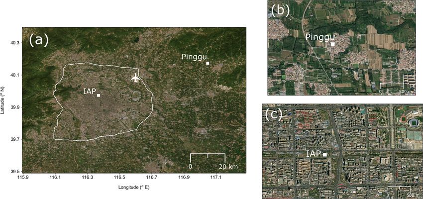
M. Biggart et al.: Modelling the canopy layer urban heat island in Beijing                                                   13689

evaluating urban climate model performance. For instance,           Lumpur (K. Wang et al., 2019). As our simulations cover the
MODIS LSTs are frequently used to evaluate the general spa-         two field campaign periods of the Atmospheric Pollution and
tial distribution of urban temperatures produced by coarse-         Human Health in a Chinese megacity (APHH-China) pro-
resolution urban climate models (Hu et al., 2014; Wouters et        gramme (Shi et al., 2019), the results may assist the inter-
al., 2016; Brousse et al., 2020).                                   pretations of related air quality measurement and modelling
   Fine-scale modelling of urban climate is regularly under-        studies (Shi et al., 2019; Biggart et al., 2020; Squires et al.,
taken to enable the testing of UHI mitigation strategies and        2020; Zhao et al., 2020). ADMS-Urban studies in London fo-
the investigation of critical issues such as how the UHI im-        cused only on specific urban developments (Hamilton et al.,
pacts heatwave events and pollution dispersion (Wang et al.,        2014) and building materials (Aktas et al., 2017), whereas in
2013; Chen et al., 2016; Fallman et al., 2016). Regional-scale      Kuala Lumpur the effects of AHEs were excluded (K. Wang
climate models, such as the Weather Research and Forecast-          et al., 2019). Several previous studies have implemented
ing model (WRF), coupled with urban canopy modules that             LCZs for UHI simulations, including in Dublin (Alexander
simulate the impact of urbanisation on climate at citywide          et al., 2015), Madrid (Brousse et al., 2016) and Singapore
scales are commonly used for these analyses (Loridan et al.,        (Mughal et al., 2019). We build on this earlier work by com-
2010; Wang et al., 2013). Higher-resolution local-scale (∼ 1        bining a LCZ map for Beijing with the locations of fine-scale
km) UHI effects can also be explored in detail with urban           green spaces, waterways and buildings from OpenStreetMap
energy balance models, such as the Surface Urban Energy             (OSM).
and Water Balance (SUEWS) model (Alexander et al., 2015),              Detailed descriptions of the ADMS-Urban model, its me-
which incorporates detailed land cover data to calculate local      teorological inputs and the development of surface param-
perturbations to surface heat fluxes (Grimmond et al., 2010).       eter and AHE datasets are provided in Sect. 2. In Sect. 3,
However, the availability of land cover information in devel-       simulated neighbourhood-scale spatiotemporal near-surface
oping countries, where heat-related mortality rates in cities       air temperature variations across urban Beijing are evaluated
are highest (Kjellstrom et al., 2009), often restricts such stud-   using in situ near-surface air temperature measurements and
ies. In fact, the Intergovernmental Panel on Climate Change’s       satellite-derived LSTs, with the impacts of extreme temper-
(IPCC) fifth assessment report specifically highlighted the         ature events on Beijing’s UHI also explored. Section 4 pro-
lack of detailed global urban land use datasets (IPCC, 2014).       vides a summary of this work’s findings, along with sugges-
Stewart and Oke’s (2012) thermal classification scheme for          tions for study improvements and future applications.
neighbourhoods, termed local climate zones (LCZs), pro-
vides one solution. It has 10 urban and 7 rural classes that can
be mapped by a variety of methods, including using remote           2     Methodology
sensing data combined with local expert-based knowledge
(Bechtel et al., 2015). LCZs are distinguished based on sur-        2.1    ADMS-Urban model description
face cover, structure, material and human activity, as they are
designed to standardise the characterisation of near-surface        The neighbourhood-scale ADMS-Urban climate model cal-
temperature measurement sites in both urban and rural loca-         culates local perturbations to vertical profiles of temperature
tions (Stewart and Oke, 2012; Ching et al., 2018).                  and humidity, representative of rural conditions upwind of
   Here we incorporate LCZ data in neighbourhood-scale              the modelled urban area, in response to spatially varying sur-
resolution (∼ 100 m) urban climate simulations across Bei-          face parameters. These upwind profiles are calculated from
jing using the ADMS-Urban Temperature and Humid-                    near-surface meteorological measurements recorded outside
ity model (hereafter, ADMS-Urban). This study aims to               the modelled urban area, ideally coinciding with air advect-
(i) quantify the relative impacts of urban surface proper-          ing towards the urban centre (i.e. upwind), and depend on the
ties and AHEs on Beijing’s canopy layer UHI during winter           planetary boundary layer height (PBLH), surface roughness
and summer periods, (ii) produce neighbourhood-scale spa-           length (z0 ) and the stability parameter PBLH/LMO . LMO is
tial distributions of near-surface air temperatures across ur-      the Monin–Obukhov length, a measure of the relative im-
ban Beijing and explore how they vary diurnally in summer,          portance of mechanical turbulence and buoyancy (Hood et
and (iii) understand the extent to which summer heatwave            al., 2018; CERC, 2020). Calculation of the local perturba-
periods affect daytime and nighttime UHIIs in Beijing.              tions to these vertical profiles arises from surface thermal and
   ADMS-Urban is chosen for this work as it can be used to          morphological parameters modifying heat and moisture pro-
capture the impact of fine-scale land cover variations on ur-       cesses, allowing a 3-D temperature and humidity field to be
ban climate, highlighting the microclimates where residents         modelled across the domain.
are most at risk from extreme temperatures and informing               The temperature and humidity perturbations are calcu-
urban planners on the cooling effects of green spaces and           lated by solving a coupled system of equations that gov-
waterways. This local-scale urban climate model has been            ern heat and moisture processes at the ground (Carruthers
used for studies in megacities of contrasting climates, such as     and Weng, 1992; Raupach et al., 1992). The conservation of
London (Hamilton et al., 2014; Aktas et al., 2017) and Kuala        heat’s boundary conditions are dependent on moisture via the

https://doi.org/10.5194/acp-21-13687-2021                                         Atmos. Chem. Phys., 21, 13687–13711, 2021
13690                                            M. Biggart et al.: Modelling the canopy layer urban heat island in Beijing

latent heat flux, and evaporative processes are temperature           al., 1999); in ADMS-Urban, this is modelled via perturba-
dependent. The equations account for the spatial variation            tions to the upwind conditions. The model accounts for the
of surface heat fluxes, moisture, mean airflow and vertical           diurnal variation of ground heat storage and release by sum-
turbulent diffusion (CERC, 2018). Heat fluxes are governed            ming the daytime storage heat flux and releasing it linearly
by variations in net radiation (Q∗ ) and storage heat, airflow        throughout the evening.
and turbulent diffusion are controlled by variations in surface          The magnitude of Q∗ − G determines the amount of en-
roughness (z0 ), and the moisture terms depend on the sur-            ergy available for partitioning between the latent (LE) and
face’s resistance to evaporation, which accounts for both sur-        sensible heat fluxes (H ). Local perturbations (1) to the up-
face wetness and sub-surface moisture, with water surfaces            wind surface heat fluxes are calculated based on relative dif-
having near-zero surface resistance to evaporation (Table 1).         ferences between upwind surface parameters defined around
   Upwind Q∗ is determined from near-surface hourly me-               the edge of the modelled urban area and the spatially vary-
teorological measurements representative of conditions up-            ing surface characteristics defined across the model domain,
wind of the model domain, following Eq. (1) (Holstag and              according to the surface energy balance equation:
van Ulden, 1983):
                                                                      1Q∗ − 1G − 1LE = 1H.                                       (3)
  ∗
Q =                                                                      The model requires the following surface parameters (Ta-
                                                                      ble 1): thermal admittance (J K−1 m−2 s−1/2 ), surface re-

(1 − r) K + − 5.67 × 10⁻⁸ T 4 + 5.31 × 10⁻¹³ T 6 + 60 C8L
                                                            ,         sistance to evaporation (s m−1 ), albedo, surface roughness
                          1.12
                                                                      length (z0 ) (m) and normalised building volume (NBV) (m).
                                                                (1)
                                                                      NBV is defined as the volume of buildings within a grid
where the first term represents the incoming SW radiation             cell per grid cell area and provides a measure of the den-
(K + ) absorbed by the surface, which is dependent on the up-         sity of buildings across the domain. Local 1Q∗ values de-
wind surface albedo (r) defined around the edge of the mod-           pend on the urban–upwind differences in albedo and NBV.
elled urban area. The second term in Eq. (1) accounts for the         1G is based on spatial differences in the surface’s thermal
LW radiation released by the surface, a function of the up-           properties (thermal admittance). Perturbations to energy lost
wind near-surface air temperature, T , and the downwelling            through evaporation at the surface (1LE) depend on locally
LW radiation from the gaseous atmosphere and cloud cover              varying surface resistance to evaporation, air temperature and
(CL ) are given by the third and fourth terms, respectively           surface moisture content. 1H represents spatially varying
(Holstag and van Ulden, 1983).                                        rates at which heat energy is transferred from the surface
   The upwind storage heat flux (G) is calculated as a func-          to the atmosphere by convection. Local perturbations to the
tion of Q∗ according to Eq. (2) (Camuffo and Bernardi,                upwind temperature profile due to surface characteristics de-
1982):                                                                pend on the cumulative effect of 1H and the local surface
                                                                      roughness length (z0 ) accounting for the impact of building
         dQ∗                                                          morphology on advection and turbulent diffusion and hence
G = a1       + a2 Q∗ + a3 ,                                     (2)
          dt                                                          heat transfer processes.
where a1 (h), a2 , and a3 (W m−2 ) are coefficients that de-          2.2   Study period and meteorological input data
pend on the land cover and surface moisture (Grimmond et
al., 1991; Grimmond and Oke, 1999) and vary sinusoidally              Simulations are performed for the winter (10 November–
throughout the year (Keogh et al., 2012; Sun et al., 2017).           10 December 2016) and summer (17 May–21 June 2017)
For this application, the coefficients selected correspond to         APHH-China measurement campaigns (Shi et al., 2019).
a hybrid of urban and rural surface properties (Grimmond              These are periods of interest given the expected impact of
and Oke, 1999) that allow for both the influence of urban             the urban canopy layer UHI on air pollution dispersion.
materials on heat exchanges as well as the advection of                 For this study, a single set of meteorological measure-
nighttime stable atmospheric conditions from the rural to ur-         ments, representing upwind conditions, are used to drive the
ban areas, with an annual mean of a1 = 0.7 h, a2 = 0.3 and            model. Near-surface air temperature and relative humidity
a3 = −7.5 W m−2 (CERC, 2018). These values represent the              (∼ 8 m a.g.l. and ∼ 50 m a.s.l.) recorded at the rural APHH-
high proportion of Q∗ absorbed into the ground during the             China field campaign site (Han, 2019) in Xibaidian village,
day in urban areas and re-released overnight, respectively,           Pinggu (40.17◦ N, 117.05◦ E) (hereafter, the rural site), are
with the asymmetry relating to the urban fabric absorbing             used along with wind speed, wind direction and cloud cover
more heat in the early part of the day and the model require-         data from the Beijing Capital International Airport Meteorol-
ment that the upwind PBLH corresponds to stable conditions            ogy Observatory. Pinggu is located ∼ 60 km north-east of the
at night. In reality, in urban areas, the nocturnal release of        urban APHH-China field site at IAP (39.97◦ N, 116.37◦ E)
stored heat is often sufficient to produce an upward convec-          (hereafter the urban site). The World Meteorological Orga-
tive heat flux and hence maintain an unstable PBL (Oke et             nization (WMO) Beijing Capital International Airport Mete-

Atmos. Chem. Phys., 21, 13687–13711, 2021                                             https://doi.org/10.5194/acp-21-13687-2021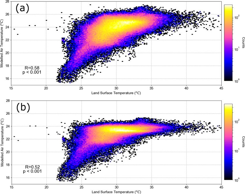
M. Biggart et al.: Modelling the canopy layer urban heat island in Beijing                                                            13691

Table 1. Surface parameter values assigned to ;local climate zones (LCZs) mapped in Beijing (WUDAPT, 2020). Values are from Stewart
and Oke (2012), except for surface resistance to evaporation. See Sect. 2.3 for a description of how values are chosen from their ranges.
Surface resistance to evaporation is based on literature-reported values (Oke, 1982; Cox et al., 1999; Hamilton et al., 2014; CERC, 2018).

               LCZ     Description             Thermal admittance               Albedo to       Surface         z0       NBV
                                                (J K−1 m−2 s−1/2 )    evaporation (s m−1 )    resistance       (m)        (m)
               1       Compact high-rise                      1650                     0.1          200           2      12.5
               2       Compact midrise                        1850                     0.1          200           1     9.625
               3       Compact low-rise                       1500                     0.1          200         0.5     3.575
               4       Open high-rise                         1600                    0.12          150           2        7.5
               5       Open midrise                           1700                    0.12          150         0.5      5.25
               6       Open low-rise                          1500                    0.12          150         0.5      1.95
               8       Large low-rise                         1500                    0.15          200        0.25        2.6
               9       Sparsely built                         1400                    0.12          150        0.25     0.975
               10      Heavy industry                         1750                    0.12          200        0.25        2.5
               A       Dense trees                            1400                    0.15          115           2     0.825
               B       Scattered trees                        1400                     0.2          115         0.5      0.45
               D       Low plants                              600                     0.2           70         0.1     0.025
               E       Bare rock or paved                     1850                   0.225          200      0.005    0.00625
               G       Water                                  1545                    0.06           10     0.0002
               Upwind domain
               Rural site (LCZ 9 modified)                     600                      0.2         150       0.25       0.975

Figure 1. Beijing and surrounding area, showing the locations of (a) the Beijing Capital International Airport Meteorology Observatory
(aeroplane), (b) the urban meteorological site at the Institute of Atmospheric Physics (IAP), and (c) the rural meteorological site in Pinggu,
with the Sixth Ring Road (white line) marking the model domain. The source of the satellite imagery is Esri World Imagery.

orology Observatory (https://ncdc.noaa.gov/, last access: 19             be less influenced by local frictional effects of neighbouring
May 2020) is situated approximately halfway between the                  small buildings and vegetation, compared to the rural site,
two sites, inside the Sixth Ring Road (Fig. 1). Measurements             due its more exposed location. Upwind vertical wind speed
of wind speed and direction from the airport site are used               profiles are perturbed locally in the model, impacting heat
as the “rural”, or upwind data, instead of those from the rural          advection, following modifications to PBL stability due to
site, as it is subject to WMO quality assurance and is likely to         spatially varying heat fluxes and surface roughness.

https://doi.org/10.5194/acp-21-13687-2021                                                Atmos. Chem. Phys., 21, 13687–13711, 2021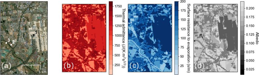
13692                                            M. Biggart et al.: Modelling the canopy layer urban heat island in Beijing

   Incorporating near-surface air temperature measurements        previous urban climate observational and numerical mod-
from a single rural meteorological station is a limitation of     elling studies. Following Ching et al. (2018), thermal ad-
this study. Ideally, we would use several rural meteorologi-      mittance values are assigned by selecting the midpoints of
cal sites distributed around the model domain, selecting the      the Stewart and Oke (2012) ranges. Estimates of surface re-
air temperature measurement from the site coinciding with         sistance to evaporation are not provided with the LCZ data;
upwind conditions; an upwind measurement is desirable so          therefore, we use literature-reported values (Oke, 1982; Cox
that the air temperature sensor is not strongly influenced by     et al., 1999; Hamilton et al., 2014; CERC, 2018). A surface
the advection of urban heat. Air temperatures measured at         resistance to evaporation of 200 s m−1 is widely deemed in
the airport site were not deemed appropriate for this study       the literature to characterise urban surfaces, and thus we as-
given that the local environment is likely heavily affected       sign it to LCZs described by Stewart and Oke (2012) as con-
by the warming effects of surrounding urban surface thermal       sisting entirely of impervious materials (LCZ 1–3, 8 and 10).
properties and nearby AHEs. For this study, the only acces-       However, to account for the high density of green spaces and
sible upwind air temperature measurement data were from           prevalence of road wetting for cleaning purposes across ur-
the rural field campaign site at Pinggu. However, during the      ban Beijing noted by Dou et al. (2019), we lower the surface
winter period, the predominant wind direction was from the        resistance to evaporation given to LCZs described by Stew-
north-east, situating the model domain downwind of the ru-        art and Oke (2012) as consisting of abundant pervious land
ral site. During the summer period, winds from the north and      cover (e.g. plants and trees) (LCZ 4–6 and 9) to 150 s m−1 ;
east are the most prevalent; however, a growing frequency of      this value is an approximate midpoint between the surface
south-westerly winds is also observed. Therefore, summer          resistance to evaporation values given to green spaces and
air temperatures measured at the rural site may be influenced     urban surfaces (Tables A1 and 1). Given the strong influence
at times by heat advection from urban Beijing.                    on daytime air temperatures of surface resistance to evap-
   At the urban site, a ceilometer gathered attenuated            oration, this adjustment is made to ensure sufficient spatial
backscatter that were analysed with the CABAM algorithm           heterogeneity in modelled air temperature is captured across
(Kotthaus and Grimmond, 2018) to provide the mixing-layer         central urban areas. The albedo values selected for each LCZ
height, the atmosphere’s lowest layer in contact with Earth’s     are the lower bounds of Stewart and Oke’s (2012) ranges,
surface resulting from turbulent exchange (Shi et al., 2019;      closely matching the literature-reported albedo values used
Hertwig et al., 2020). This was assumed to equate to the          for the OSM data. Surface roughness lengths (z0 ) correspond
PBLH.                                                             with the Davenport classes Davenport et al. (2020) assigned
                                                                  to each LCZ by Stewart and Oke (2012). The NBV are cal-
2.3   ADMS-Urban surface parameters                               culated as the product of the midpoints of Stewart and Oke’s
                                                                  (2012) ranges for roughness element height and building sur-
Near-surface air temperatures are modelled across the area        face fraction.
contained within Beijing’s Sixth Ring Road (Fig. 1); the reso-       A spatially weighted mean of the surface parameters is cal-
lution of the model calculation grid is ∼ 105 m. Thermal and      culated at 100 m resolution (Fig. 3), matching the resolutions
morphological properties covering the modelled urban area         of the LCZ data and the model calculation grid (∼ 105 m).
and surrounding suburban regions are derived from Open-           Surface characteristics at the upwind meteorological site are
StreetMap (OSM) data (https://openstreetmap.org/, last ac-        represented by a 1 km border extending around the perime-
cess: 9 March 2020) and LCZs mapped by the World Ur-              ter of each thermal and morphological surface parameter
ban Database and Access Portal Tools (WUDAPT) project             map in Fig. 3. Differences between upwind surface param-
(http://www.wudapt.org/cities/in-asia/, last access: 19 May       eters and those within the model domain are used to cal-
2020). The function and plan area of specific buildings, green    culate the urban temperature perturbations (Sect. 2.1). The
spaces and waterways are obtained from OSM (Fig. 2). Ta-          surface information defined between the Sixth Ring Road
ble A1 provides a full list of the OSM land use types and         and the 1 km upwind border (Fig. 3), covering suburban
the thermal admittance, surface resistance to evaporation and     areas, is required in the model to prevent erroneous sim-
albedo values assigned to each, based on data reported in the     ulated temperatures associated with a sharp transition be-
literature (Oke, 1982; Cox et al., 1999; Hamilton et al., 2014;   tween urban and rural surface parameters. Upwind param-
CERC, 2018; K. Wang et al., 2019).                                eters (Table 1) were derived from Stewart and Oke’s (2012)
   OSM land use information is overlaid onto Beijing’s LCZ        ranges for LCZ 9 based on its definition as a “natural set-
classes, which are mapped at 100 m resolution (Fig. 2). The       ting with sparsely arranged buildings and abundant pervious
methodology for generating LCZ maps for specific cities           land cover”, closely matching the environment at the rural
is well-documented (Stewart and Oke, 2012; Bechtel et al.,        site in Pinggu (Shi et al., 2019). Stewart and Oke’s (2012)
2015; Ching et al., 2018). For Beijing, there are nine urban      LCZ 9 parameter values were modified to those given in Ta-
and six rural LCZ types (Fig. 2; Table 1). The surface param-     ble 1 following model sensitivity tests, with thermal admit-
eters assigned to each LCZ (Table 1) are based on ranges of       tance most notably reduced to 600 J K−1 m−2 s−1/2 , account-
values suggested by Stewart and Oke (2012), derived from          ing for the large increment of heat stored in Beijing’s urban

Atmos. Chem. Phys., 21, 13687–13711, 2021                                         https://doi.org/10.5194/acp-21-13687-2021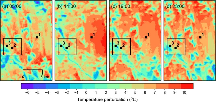
M. Biggart et al.: Modelling the canopy layer urban heat island in Beijing 13693
Figure 2. Sources of data used to determine model surface parameters for Beijing, covering the model domain within the Sixth Ring Road
(red line), including (a) OpenStreetMap (OSM, 2020) land use (Table A1) and (b) local climate zones (LCZ) (WUDAPT, 2020). OSM land
use overlaid onto LCZs across central Beijing (black square in b) is shown in (c), with the urban meteorological site at the Institute of
Atmospheric Physics (IAP) also marked. © OpenStreetMap contributors 2020. Distributed under the Open Data Commons Database License
(ODbL) v1.0.
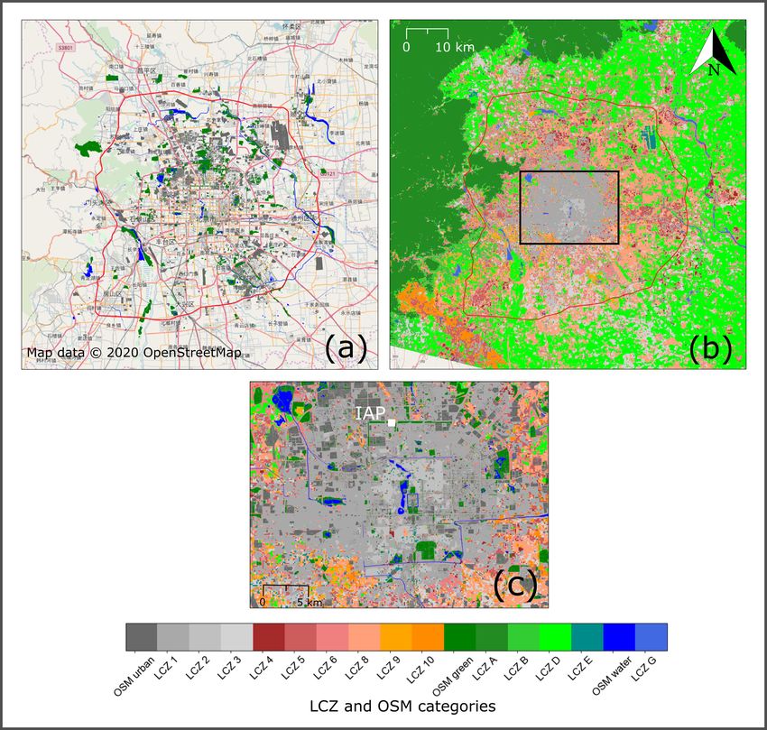
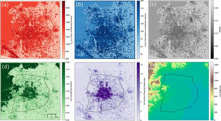
fabric relative to neighbouring rural areas. Altitude effects 2.4 Anthropogenic heat emissions (AHE)
on temperature are accounted for with the use of terrain el-
evation data (Fig. 3f) (https://www.usgs.gov/land-resources/ The anthropogenic heat flux is not included in Eq. (3) and
eros/coastal-changes-and-impacts/gmted2010, last access: 1 needs to be accounted for. The main sources include power,
April 2020). Urban Beijing is situated on a plain at an alti- industry, transportation, residential and commercial building
tude of ∼ 50 m, but mountainous terrain lies to the north and use, and human metabolism (Sailor, 2011; Lu et al., 2016;
west of the city across the rural areas (Fig. 3f). Yu et al., 2018). Our values are based on a mean summer
AHE value estimated by Dou et al. (2019) at IAP using the
https://doi.org/10.5194/acp-21-13687-2021 Atmos. Chem. Phys., 21, 13687–13711, 2021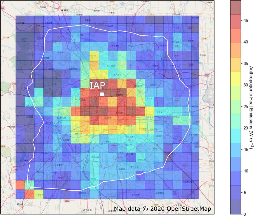
13694                                                 M. Biggart et al.: Modelling the canopy layer urban heat island in Beijing

Figure 3. Surface characteristics in the Beijing area (100 m resolution) showing the Sixth Ring Road (white or black line), including (a) ther-
mal admittance (J K−1 m−2 s−1/2 ), (b) surface resistance to evaporation (s m−1 ), (c) albedo, (d) surface roughness length (z0 ) (m), (e) nor-
malised building volume (NBV) (m) and (f) terrain elevation (USGS, 2020). See Sect. 2.3 for data sources and the method used for deter-
mining parameter values.

Large scale Urban Consumption of Energy model (LUCY)                      is the summer (June, July and August) mean AHE calcu-
(Lindberg et al., 2013). Their daily mean aggregate summer                lated for IAP by Dou et al. (2019), and MSFJJA gives the
AHE (48.1 W m−2 ) is derived from national- and provincial-               mean scaling factor for summer months (Fig. 5). A spatially
level energy consumption data and spatial proxy information               weighted mean of the LCZ-specific AHEs is calculated at
(population density, gross domestic product and vehicle own-              3 km resolution (Fig. 4).
ership rates) (Dou et al., 2019), a methodology also applied                 Single diurnal and monthly profiles are applied to the
to other worldwide megacities, such as London (Gabey et                   AHEs based on the profiles estimated by Lu et al. (2016).
al., 2019) and Shanghai (Ao et al., 2018). For this study, we             Lu et al. (2016) derived annual sectoral AHE totals for all
generate a 3 km resolution grid (Fig. 4) of aggregate AHEs,               provinces and municipalities in China from the officially
representing the sum of all AHE source sectors. First, the                published energy consumption statistics, obtained from a va-
IAP value for summer (mean for June, July and August)                     riety of sources (e.g. China Energy Statistical Yearbook).
is scaled to represent an annual mean AHE value based on                  Weighted means of the diurnal and monthly temporal profiles
literature-reported monthly scaling factors (Fig. 5) (Lu et al.,          for each sector, from Lu et al. (2016), are determined in rel-
2016). This annual mean AHE for IAP is distributed spatially              ative proportion to the total annual sectoral AHEs estimated
through further scaling by the magnitudes of AHE estimated                for the Beijing municipality. The nocturnal contribution from
for each LCZ class by Stewart and Oke (2012) relative to the              transportation is increased, following Biggart et al. (2020),
AHE value for LCZ 1 (IAP is situated in LCZ 1), according                 to account for the influx of heavy-duty diesel trucks (HD-
to Eq. (4):                                                               DTs) into urban Beijing after the daytime ban (06:00–23:00)
                                                                          within the Fourth Ring Road (Zhang et al., 2019). We as-
          Xi   YJJA                                                       sume approximate direct proportionality between air pollu-
AHEi =       ×      ,                                            (4)
          X1 MSFJJA                                                       tant emissions (Biggart et al., 2020) and AHEs from HDDTs
                                                                          and increase the nocturnal transportation sector AHE com-
where AHEi is the annual mean AHE value for LCZi (i =                     ponent, estimated by Lu et al. (2016), by ∼ a factor of 2.
11–15 for LCZ A, B, D, E and G, respectively). Xi and                        The resulting monthly and diurnal aggregate AHE profiles
X1 represent the AHE value estimated by Stewart and Oke                   (Fig. 5) have winter and summer peaks primarily caused by
(2012) for LCZi and 1 (midpoint of range), respectively. YJJA

Atmos. Chem. Phys., 21, 13687–13711, 2021                                                   https://doi.org/10.5194/acp-21-13687-2021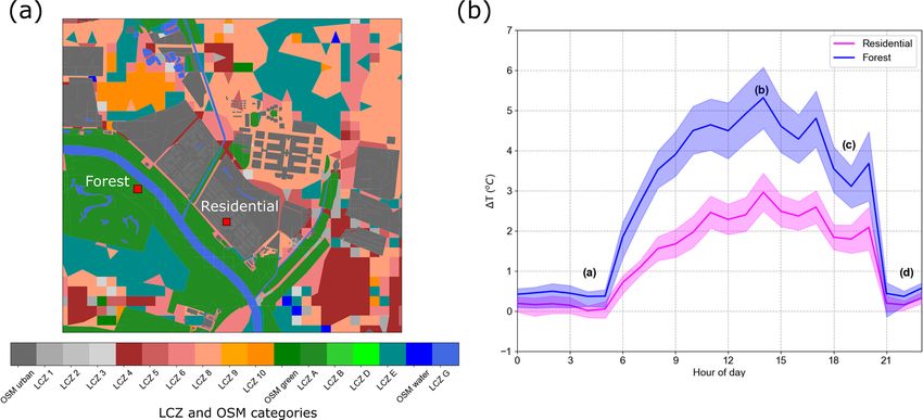
M. Biggart et al.: Modelling the canopy layer urban heat island in Beijing                                                     13695

                                                                     2.5   Model evaluation

                                                                     The magnitude and temporal variability of Beijing’s win-
                                                                     ter and summer canopy layer UHI are evaluated using
                                                                     hourly near-surface air temperature measurements. Unlike
                                                                     city-scale urban climate modelling studies, which commonly
                                                                     compare regional-scale climate model output with the near-
                                                                     est meteorological measurement station to a model grid box
                                                                     (Chen et al., 2016, 2018; Fallmann et al., 2016), ADMS-
                                                                     Urban can simulate air temperatures at specific locations cor-
                                                                     responding to the exact coordinates of measurement sites.
                                                                     We compare UHIIs modelled at the urban site at IAP, for
                                                                     the winter and summer periods, with measured UHIIs, cal-
                                                                     culated as the difference between near-surface air tempera-
                                                                     tures observed at the urban and rural sites. Air temperatures
                                                                     at the urban site are recorded at ∼ 8 m a.g.l. and ∼ 50 m a.s.l.,
                                                                     matching the measurement height and terrain elevation of the
                                                                     temperature sensor at the rural site (Sect. 2.2). The following
Figure 4. Aggregate anthropogenic heat emissions (AHEs) (3 km        statistical performance measures are used for model evalua-
resolution) across Beijing. Magnitudes based on Dou et al. (2019)    tion:
with spatial weightings based on the local climate zone (LCZ) lo-
cations (Fig. 2) and Stewart and Oke’s (2012) AHE values for each    root-mean-square error (RMSE) :
LCZ classification. The Sixth Ring Road and urban meteorological        v
                                                                        u n
site (IAP) are marked. © OpenStreetMap contributors 2020. Dis-          u1 X
                                                                      =t         (Oi − Mi )2 ;                                    (6)
tributed under the Open Data Commons Database License (ODbL)               n i=1
v1.0.
                                                                                                 M−O
                                                                     fractional bias (Fb) :=             ;                        (7)
                                                                                            0.5(O + M)
elevated heating and cooling activities, respectively, in res-       Pearson’s correlation coefficient (R) :
idential and commercial buildings (Ichinose et al., 1999).                                                 !
Emissions are assumed to be proportional to electricity and               1 Xn               M             O
                                                                     =           i=1
                                                                                       Mi −         Oi −       ;                  (8)
heating fuel consumption (Lu et al., 2016). Elevated day-               n−1                 σM            σO
time AHEs with late morning and early evening peaks are
predominantly from the combination of daytime commercial             where n denotes the total number of matching hourly mod-
building thermal regulation and residential cooking and heat-        elled (M) and observed (O) UHIIs, M and O indicate mean
ing, with a smaller contribution from rush-hour-related traffic      modelled and observed UHIIs, respectively, and σ is the stan-
volume maxima (Lee et al., 2009; Ao et al., 2018).                   dard deviation.
   AHEs are modelled as individual plumes with the ADMS-                Further measured–modelled air temperature comparisons
Urban air quality model (Owen et al., 2000; CERC, 2018)              are not possible due to a lack of access to other near-
and build upon the local temperature perturbations caused            surface air temperature observations. However, satellite-
by spatially varying surface characteristics (Sect. 2.1). All        derived LSTs are readily available for the Beijing area and,
AHEs are assumed to be released into the atmosphere and              although the ADMS-Urban model does not calculate LST,
then dispersed assuming quasi-Gaussian distributions driven          the correlation between neighbourhood-scale spatial varia-
by the upwind meteorological variables, the PBLH and the             tions of modelled near-surface air temperature and satellite-
PBLH/LMO stability parameter. The accumulation of dis-               derived LST provides a useful comparison for model eval-
persed plumes of anthropogenic heat gives an energy density          uation. This technique was also adopted by K. Wang et
field (CT ), in units of J m−3 , which is converted to a local air   al. (2019) for high-resolution UHI simulations across Kuala
temperature increment (1T ) in the model according to                Lumpur using ADMS-Urban to assist in the evaluation of
                                                                     modelled near-surface air temperature spatial patterns. Land-
                                                                     sat 8 Operational Land Imager (OLI)/Thermal Infrared Sen-
       CT
1T =       ,                                                  (5)    sor (TIRS) thermal band TIRS-1 data (https://www.usgs.gov/
       ρcp                                                           land-resources/nli/landsat, last access: 1 April 2020) are ac-
                                                                     quired at 100 m resolution, matching the modelled spatial
where ρ (1.225 kg m−3 ) and cp (1012 kJ kg−1 K−1 ) are stan-         resolution. LSTs are retrieved using the single-channel algo-
dard values for the density and specific heat capacity of air at     rithm developed by Jiménez-Muñoz et al. (2009). We focus
15 ◦ C (CERC, 2018).                                                 on the summer for this analysis given the stronger incoming

https://doi.org/10.5194/acp-21-13687-2021                                          Atmos. Chem. Phys., 21, 13687–13711, 2021
13696                                               M. Biggart et al.: Modelling the canopy layer urban heat island in Beijing

Figure 5. (a) Diurnal and (b) monthly anthropogenic heat emission (AHE) profiles. See Sect. 2.4 for a description of how the profiles were
determined.

SW, compared to winter, and hence the expected more a di-              et al., 2019), the surface resistance to evaporation values are
rect relationship between LSTs and near-surface air temper-            reduced to 150 s m−1 in LCZ categories 1–3, 8 and 10 (Ta-
atures (K. Wang et al., 2019), with near-surface air temper-           ble 1), as well as for all urban OSM land use types (Table A1)
atures strongly influenced by the upwards flux of heat from            for the Evp150 case (Table 2). This matches the surface re-
the surface. Landsat 8 LSTs are available for 23 May 2017              sistance to evaporation assigned to the upwind domain. The
at 10:53 LT (local time), a time with minimal cloud cover,             noAHE case is designed to isolate the contribution to Bei-
and are compared with near-surface air temperatures simu-              jing’s UHI from land surface characteristics alone, and thus
lated on the same day at 11:00 LT, with both sampled on the            AHEs are excluded.
same 100 m resolution grid. LSTs are compared with simula-
tions that exclude AHEs for the following reasons: (i) previ-
ous studies have reported difficulties in determining the im-          3     Results and discussion
pact of AHEs on LSTs (Kato and Yamaguchi, 2005; Wang
et al., 2017), and (ii) micro-scale advection of heat released         First, we evaluate UHIIs simulated at the urban site for the
by nearby surfaces is known to uncouple LSTs and air tem-              winter and summer periods (Sect. 3.1). The neighbourhood-
peratures (Roth et al., 1989; Voogt and Oke, 1998); thus, we           scale spatial variations of modelled near-surface air temper-
expect the release of anthropogenic heat to have a similarly           atures are assessed using satellite-derived LSTs in Sect. 3.2.
strong influence on near-surface air temperatures and further          Section 3.3 investigates the extent to which spatial tempera-
contribute to differences with spatial LST variability.                ture patterns vary throughout the day, focussing on the spa-
                                                                       tiotemporal characteristics of neighbouring (but distinctly
2.6   Model experiments                                                different) urban microclimates. Summer heatwave events are
                                                                       identified in Sect. 3.4 and their impact on Beijing’s UHI is
We perform simulations with four distinct model configura-             discussed.
tions, each involving different surface property or AHE sce-
narios (Table 2). The experiments are designed to identify             3.1    Model evaluation of diurnal UHII in winter and
how the modelled UHII can be optimised to best represent                      summer
the observations by use of appropriate input parameters, thus
providing insight into the key processes driving Beijing’s             The winter and summer period mean observed canopy layer
UHI in winter and summer. The base case uses the initial               UHIIs (IAP-Pinggu) are 3.1 and 1.8 ◦ C, respectively. These
surface parameters and AHEs (Sect. 2.3 and 2.4). Gabey et              values are similar to those derived previously from a dense
al. (2019) showed that the top-down approach for estimating            network of ground measurements in Beijing (Yang et al.,
AHEs, as used for the AHEs adopted for this study, tends               2013; Wang et al., 2017). Yang et al. (2013) reported win-
to underestimate hotspots associated with dense inner-city             ter and summer averages across central Beijing (within the
road networks and compact building developments. There-                Fourth Ring Road) of 2.4 and 1.5 ◦ C, respectively. Base case
fore, base case AHE values are increased by 50 % in the                simulated UHIIs are underestimated for both periods com-
AHE50 case (Table 2). Given the unexpectedly high latent               pared to the measurements, with the winter values less than
heat flux values measured previously at the IAP site (Dou              half the observed UHIIs (RMSE = 2.90 and Fb = −0.76; Ta-

Atmos. Chem. Phys., 21, 13687–13711, 2021                                                https://doi.org/10.5194/acp-21-13687-2021
M. Biggart et al.: Modelling the canopy layer urban heat island in Beijing 13697
Table 2. Surface parameters and anthropogenic heat emissions (AHEs) used in the four model experiments.
Case Surface parameters AHEs
Base As in Tables 1 and A1 As Figs. 4 and 5
AHE50 Base Base +50 %
Evp150 Base with Evp (LCZ 1–3, 8, 10 and urban OSM) = 150 s m−1 Base +50 %
noAHE Base with Evp (LCZ 1–3, 8, 10 and urban OSM) = 150 s m−1 0
ble 3). The summer underestimation is lower; however, the rise buildings (Fig. 1), both of which are likely strong sources
RMSE is proportionally higher (Table 3). of anthropogenic heat, with nearby buildings also hindering
The UHI is known to have distinct diurnal characteristics the dispersion of heat at night. Two of the four urban me-
(Oke et al., 2017), and thus analysis of the model’s ability to teorological stations in Beijing used by Wang et al. (2017)
simulate the diurnal UHII variation can inform on the daily are situated in green belts or parks, and thus they are likely
varying contributions to urban climate perturbations from to be less influenced by major local sources of AHEs, which
surface energy balance changes, AHEs and background me- may account for the lower nocturnal UHIIs observed there
teorology. Measured UHIIs in winter and summer peak dur- relative to IAP. Additionally, Cao et al. (2016) found a strong
ing the evening at ∼ 4.5 ◦ C (Fig. 6). However, other studies correlation between high concentrations of particulate matter
have found Beijing’s canopy layer UHII maximum to be up over urban areas and the nocturnal UHI for several megaci-
to a factor of 2 greater in winter compared to summer months ties in China due to enhanced atmospheric absorption and
(Liu et al., 2007; Wang et al., 2017). They attributed this to re-emission of LW radiation back to the surface, reducing
stronger winter AHEs from elevated energy consumption for the evening cooling rate. The ADMS-Urban radiation model
building heating systems (Lu et al., 2016), which readily ac- does not account for nocturnal warming effects from haze
cumulate in Beijing’s frequently stable and shallow winter pollution, which has been shown to change surface energy
nocturnal boundary layer (Zhang et al., 2016), and more ef- and water partitioning in Beijing (Kokkonen et al., 2019).
ficient nocturnal cooling in rural areas under frequent strong Summer UHII underestimations at night, relative to mea-
winter temperature inversions (Yang et al., 2013). Summer- surements, are similarly reduced by ∼ 0.6 ◦ C with increased
time nocturnal UHIIs are influenced more by the delayed re- AHEs (Table 4; Fig. 6b), reflected by a fractional bias im-
lease of heat stored within the urban fabric throughout the provement from −0.61 to −0.4 (Table 4). The remain-
day (Oke et al., 1999; Wang et al., 2013), with a smaller pro- ing measured–modelled discrepancy is likely related to the
portion attributed to AHEs from residential air conditioning model’s determination of nocturnal ground heat flux, with
units (Zhao et al., 2018). the restriction that modelled upwind PBL conditions remain
Simulated evening UHII maxima are underestimated com- stable at night (CERC, 2018). However, the evening release
pared to measurements for all scenarios, with base case of stored heat in other dry, densely built megacities in sum-
values ∼ 2.5 ◦ C lower than measurements from 19:00 to mer, such as Mexico City (Oke et al., 1999), has been found
06:00 LT in winter and ∼ 2 ◦ C lower between 21:00 and to be of sufficient magnitude to maintain an upward flux of
04:00 LT in summer (Fig. 6). However, previous studies of convective heat throughout the evening, therefore prolonging
Beijing’s evening canopy layer UHI in summer measured the warming of near-surface air.
at different central urban meteorological sites have reported The lowest measured urban–rural near-surface air temper-
mean values between 2 and 3 ◦ C (Yang et al., 2013; Wang et ature differential occurs between 13:00 and 14:00 LT in both
al., 2017; Jiang et al., 2019), agreeing closely with our sim- the winter and summer periods (Fig. 6). In summer, the ob-
ulated results (Table 4; Fig. 6b). This suggests that Beijing’s served mean UHII minimum is negative (−1.1 ◦ C). Daytime
canopy layer UHI exhibits strong spatial variability and that UHIIs are largely controlled by the balance between (i) the
our local site characteristics at IAP may be incorrect. urban–rural evapotranspiration differences based on vegeta-
Increasing AHEs by 50 % reduces nocturnal measured– tion amounts and irrigation behaviour in both areas (Oke et
modelled discrepancies in winter by ∼ 0.7 ◦ C (Table 4; al., 1982; Grimmond et al., 1993; Estoque et al., 2017; He
Fig. 6a). However, a substantial model underestimation per- et al., 2020) and by (ii) the large storage heat fluxes associ-
sists (∼ 2 ◦ C), with nighttime RMSE and fractional bias val- ated with the building volumes and impervious materials of
ues of 3.11 ◦ C and −0.58, respectively (Table 4). These low high thermal conductivity and heat capacity in urban areas
simulated nocturnal UHIIs are likely related to the use of (Anandakumar, 1999; Grimmond and Oke, 1999; Oke et al.,
coarse-resolution (3 km) aggregate AHEs that fail to resolve 1999). Dry or limited vegetation will increase the UHII, but
strong, local emission sources around the urban site at IAP. urban structures and materials can both shade and enhance
The IAP temperature sensor is located ∼ 110 m south of a storage heat fluxes, leading to delayed turbulent heat fluxes
busy road (Biggart et al., 2020) and is surrounded by high- and decreasing the urban near-surface temperatures. Nega-
https://doi.org/10.5194/acp-21-13687-2021 Atmos. Chem. Phys., 21, 13687–13711, 202113698 M. Biggart et al.: Modelling the canopy layer urban heat island in Beijing
Table 3. Statistical evaluation of modelled urban heat island intensities (UHIIs) at the urban site, for all hours of the day, during the winter
(W) and summer (S) periods. Model experiments are described in Sect. 2.5. Mean UHIIs and statistics are calculated from matching hourly
values.
UHII (◦ C) Model evaluation statistics
Observed Modelled RMSE (◦ C) Fb R
W S Case W S W S W S W S
3.1 1.8 Base 1.4 1.3 2.90 2.66 −0.76 −0.30 0.47 0.48
AHE50 2.0 1.8 2.69 2.69 −0.43 −0.02 0.39 0.44
Evp150 1.9 1.2 2.68 2.49 −0.48 −0.44 0.43 0.59
noAHE −0.1 −0.2 4.05 3.07 −2.00 −2.00 0.62 0.76
Table 4. Statistical evaluation of modelled urban heat island intensities (UHIIs) for the winter (W) and summer (S) periods (as in Table 3)
for daytime (D) (simulated K+ > 0) and night-time (N) hours.
UHII (◦ C) Model evaluation statistics
Observed Modelled RMSE (◦ C) Fb R
W S Case W S W S W S W S
D N D N D N D N D N D N D N D N D N D N
Base 0.9 1.7 0.7 2.3 1.62 3.45 2.27 3.19 −0.24 −0.86 1.01 −0.61 0.31 0.30 0.31 −0.01
1.1 4.3 0.2 4.3 AHE50 1.4 2.4 1.1 2.9 1.85 3.11 2.41 3.10 0.21 −0.58 1.26 −0.40 0.30 0.22 0.31 −0.04
Evp150 1.2 2.3 0.2 2.7 1.71 3.12 1.99 3.14 0.04 −0.59 −0.17 −0.46 0.36 0.22 0.52 −0.03
noAHE −0.4 0.1 −0.9 0.8 2.13 4.85 2.25 4.05 −2.00 −1.95 −2.00 −1.39 0.57 0.20 0.61 0.29
tive afternoon UHIIs previously observed in Beijing (Wang ferences (< 0.2 ◦ C) occur in modelled winter UHIIs between
et al., 2017) were ascribed to a substantial discrepancy be- AHE50 and Evp150 cases, in contrast with substantial re-
tween urban and rural measurement heights, but this is not a ductions to all values (0.5–1.5 ◦ C) in summer (Fig. 7). Fur-
factor here (Sect. 2.2 and 2.5). thermore, the simulated diurnal temperature range in summer
Modelled daytime UHIIs with elevated AHEs exceed the without AHEs (noAHE case) is 3 times higher than in win-
observed values (∼ 0.3 ◦ C in winter and ∼ 0.9 ◦ C in sum- ter (∼ 2.5 ◦ C) (Fig. 6), driven by much stronger incoming
mer, Table 4; Fig. 6). However, previously observed daytime SW radiation, which enhances the urban–rural differences
UHIIs in central Beijing at multiple meteorological stations between available energy partitioning and therefore impacts
(Yang et al., 2013; Jiang et al., 2019) are of similar magnitude all of the surface energy balance fluxes (Eq. 3).
to the AHE50 case values. The model’s inability to replicate Differences between UHIIs simulated with and without
the negative daytime UHIIs observed at the urban site may AHEs (both cases with high urban moisture levels) quantify
be due to an underestimation of afternoon storage heat flux the diurnally averaged and hourly AHE contributions to the
or possibly that there are nearby fine-scale green spaces, un- UHI in winter and summer (Figs. 6 and 7). These results sug-
resolved in the land cover data implemented for this study, gest that Beijing’s urban warming in winter is dominated by
that increase evaporative cooling at IAP and limit its repre- AHEs, with a small contribution from surface radiative ef-
sentativeness of the central Beijing region. fects alone between −0.5 and +0.1 ◦ C. In summer, AHEs
Model predictions of summer afternoon UHIIs are im- increase the modelled UHII by ∼ 60 %–80 % throughout the
proved when urban surface resistance to evaporation is re- day (Fig. 6), peaking at 84 % at 20:00 LT, associated with
duced from 200 to 150 s m−1 (Evp150 case), with cooler ur- heat released from residential cooling systems and rush hour
ban air temperatures simulated as the latent heat flux (Eq. 3) traffic (Fig. 5) accumulating in a stabilising evening PBL
is increased (R = 0.52; Fb = −0.17; Table 4). High moisture (Shi et al., 2019; Hertwig et al., 2020). Wang et al. (2013)
availability in central Beijing (i.e. low Bowen ratio, where simulated a similar daily maximum AHE contribution to the
Bowen ratio = sensible heat flux/latent heat flux) and specif- UHI in Beijing of 75 %. Excluding AHEs causes winter and
ically at IAP, has previously been observed (Dou et al., 2019) summer UHII biases to grow (RMSE of 4.05 and 3.07, re-
and is thought to be related to extensive use of water for road spectively), whereas the temporal variations become more
cleaning and for irrigating the high density of greenbelts in similar (R = 0.62 and 0.76 in winter and summer, respec-
urban Beijing. Smaller decreases in simulated daytime tem- tively; Table 3), reflected by the increased linearity between
perature in winter, after increasing urban moisture levels, are observed and noAHE modelled UHIIs in Fig. 7. Substan-
due to weak levels of incoming SW radiation. Negligible dif- tially larger error bars associated with both simulations that
Atmos. Chem. Phys., 21, 13687–13711, 2021 https://doi.org/10.5194/acp-21-13687-2021M. Biggart et al.: Modelling the canopy layer urban heat island in Beijing 13699 Figure 6. Mean diurnal variation in measured and modelled urban heat island intensities (UHIIs) at the urban site in (a) winter and (b) sum- mer. Modelled UHIIs from the base (dotted black), anthropogenic heat emissions +50 % (AHE50; dashed black), high urban moisture (Evp150; blue) and anthropogenic heat emissions excluded (noAHE; pink) cases are presented. Measurements are marked by the red line. Shaded regions and error bars represent the 95 % confidence intervals for modelled and measured UHIIs, respectively. Figure 7. Hourly measured and modelled urban heat island intensities (UHIIs) for (a) winter and (b) summer periods. Modelled UHIIs from the high urban moisture (Evp150; blue), anthropogenic heat emissions +50 % (AHE50; grey) and anthropogenic heat emissions excluded (noAHE; pink) cases are presented. Measured UHIIs are grouped into bins (0.5 ◦ C), points representing the mean modelled UHII are in the bin. Point sizes are scaled by total number of hourly values per bin. Error bars represent 1 SD (standard deviation) of hourly modelled UHIIs in each bin. include AHEs are related to increased measured–modelled useful for urban planners. Most notably, our results suggest differences caused by simulated and real-world PBL dynam- that strategies aimed at reducing the daytime storage heat ics differences and subsequent impacts on modelled heat dis- flux would help to decrease nighttime UHIIs in summer by persion. reducing nocturnal heat release, hence lowering the cooling Quantifying the relative importance of urbanisation- energy demand at night and therefore the contribution from induced surface energy balance changes, including AHEs, is AHEs to urban warming. https://doi.org/10.5194/acp-21-13687-2021 Atmos. Chem. Phys., 21, 13687–13711, 2021
13700                                             M. Biggart et al.: Modelling the canopy layer urban heat island in Beijing

3.2   High-resolution spatial temperature variations in            the Sixth Ring Road (Fig. 8a and b). This spatial variation is
      summer                                                       greater during the early evening hours (not shown), when the
                                                                   canopy layer UHI peaks (Fig. 6b) with more clearly defined
Maps of near-surface air temperature provide information on        near-surface temperature hotspots.
the location and physical characteristics of the warmest urban        Correlation between the spatial variation of LSTs and sim-
microclimates that may pose the biggest health risk to resi-       ulated near-surface air temperature improves when using the
dents during extreme heat events. Urban cool islands (higher       base case surface resistance to evaporation values (R = 0.58)
rural versus urban temperatures) associated with waterways         relative to the high urban moisture case (R = 0.52; Fig. 9).
and green spaces (K. Wang et al., 2019) can also be identi-        This is caused by modelled air temperature increases within
fied.                                                              the Fifth Ring Road of 2 to 3 ◦ C (Fig. 8c) as a result of re-
   Neighbourhood-scale resolution (∼ 100 m) maps of sim-           duced daytime evaporative cooling. Near-surface air temper-
ulated air temperature (2.5 m a.g.l.) across urban Beijing on      atures simulated with high urban moisture do not have the
23 May 2017 at 11:00 LT are compared with Landsat 8 LSTs           same general decrease with distance from the urban centre
(Sect. 2.5) in Fig. 8. Due to the infrequency of Landsat 8         as seen in the LSTs (Fig. 8) because the spatial variability in
satellite image availability (every 16 d), we are unable to test   the surface resistance to evaporation has been removed. This
how variable the spatial correlation between LSTs and mod-         is reflected in Fig. 9b, with no relationship between the high-
elled near-surface air temperatures is with time. However, the     est LSTs and Evp150 case simulated air temperatures. Equal
comparison for this single hour during the summer period           urban and upwind surface resistance to evaporation values
provides a useful guide for assessing the general model per-       (150 s m−1 ) lead to simulated central urban air temperatures
formance in capturing urban Beijing’s neighbourhood-scale          that are mainly controlled by the much greater thermal admit-
air temperature patterns using a hybrid of LCZ and OSM             tance values across the modelling domain versus the upwind
land cover data. Near-surface temperatures are modelled with       domain. This lowers central urban near-surface air temper-
base and Evp150 case surface resistance to evaporation val-        atures at 11:00 LT relative to suburban regions between the
ues (AHEs excluded) to test the representativeness of the en-      Fifth Ring Road and Sixth Ring Road that have lower ther-
hanced urban moisture scenario for the full model domain.          mal admittances (Fig. 2), producing a homogeneous urban
   Generally, the range of LSTs far exceeds that of near-          near-surface air temperature distribution (Fig. 8b). This is a
surface air temperatures across urban areas. Large differ-         further indication that local surface radiative cooling, likely
ences in thermal properties between impervious surfaces            due to nearby green spaces, differentiates the urban site from
and the atmosphere and different heating mechanisms cause          the mean conditions across the central Beijing region. Worse
LSTs to heat more rapidly in response to the absorption at the     spatial correlation with LSTs but better agreement with near-
surface of strong incident SW radiation in summer, whereas         surface air temperature measurements with increased urban
the atmosphere heats by convection (Anandakumar, 1999).            moisture also reflects expected differences between LSTs
Differences between LSTs and air temperatures vary diur-           and near-surface air temperatures. Micro-scale advection and
nally, with the Landsat overpass time (11:00 LT) coinciding        turbulent diffusion within the urban canopy can mix warmer
with an atmospheric urban cool island in summer (Fig. 6b)          and cooler pockets of air, reducing the coupling between
but also a growing surface urban heat island that peaks in the     LSTs and air temperatures (Roth et al., 1989).
early afternoon (Meng et al., 2018; Li et al., 2020). Further-        The lowest LSTs and modelled air temperatures correlate
more, air temperatures within the urban canopy are impacted        most strongly (Fig. 9), corresponding with green spaces, wa-
by all of the energy exchange processes, including micro-          terways (Fig. 2) and areas of high elevation (Fig. 3). The
scale advection of heat from nearby surfaces with vary-            model’s ability to capture these fine-scale urban cool islands,
ing moisture content, thermal properties and aerodynamic           such as Qianhai Lake near the centre of Beijing (Fig. 2), in
roughness, and thus they can become uncoupled from the             addition to the general urban temperature pattern, highlights
LSTs (Voogt and Oke, 2003). These inherent differences be-         the successful implementation for this study of the LCZ and
tween the two variables limit direct comparisons and thus the      OSM data.
strength of the correlation to be expected; however, the rela-
tive spatial patterns are of interest.                             3.3   Spatiotemporal UHI variations near the airport
   The LSTs range between 16 and 47 ◦ C within the domain
(Fig. 8). They generally peak within the Fifth Ring Road and       Large-scale urban developments strongly impact local air
decrease with distance from the urban centre as the amount         temperatures, following the replacement of vegetative sur-
of green space increases (Estoque et al., 2017). Small areas       faces with expanses of concrete and asphalt, and therefore
of high LSTs in suburban zones between the Fifth Ring Road         affect the thermal comfort, cooling and heating energy de-
and Sixth Ring Road to the NW and SE (Fig. 8d) are re-             mand, and air quality across neighbouring residential areas
flective of the suburban expansion during the last decade ob-      (Hamilton et al., 2014). In this section, we investigate the
served by Liu et al. (2020). The modelled near-surface air         extent to which simulated spatial temperature patterns near
temperatures at 11:00 LT range between 15 and 27 ◦ C within        the Beijing Capital International Airport vary throughout the

Atmos. Chem. Phys., 21, 13687–13711, 2021                                          https://doi.org/10.5194/acp-21-13687-2021
You can also read