Spatial and temporal variability in the hydroxyl (OH) radical: understanding the role of large-scale climate features and their influence on OH ...
←
→
Page content transcription
If your browser does not render page correctly, please read the page content below
Atmos. Chem. Phys., 21, 6481–6508, 2021
https://doi.org/10.5194/acp-21-6481-2021
© Author(s) 2021. This work is distributed under
the Creative Commons Attribution 4.0 License.

Spatial and temporal variability in the hydroxyl (OH) radical:
understanding the role of large-scale climate features and their
influence on OH through its dynamical and photochemical drivers
Daniel C. Anderson1,2 , Bryan N. Duncan2 , Arlene M. Fiore3 , Colleen B. Baublitz3 , Melanie B. Follette-Cook2,4 ,
Julie M. Nicely2,5 , and Glenn M. Wolfe2
1 UniversitiesSpace Research Association, GESTAR, Columbia, MD, USA
2 Atmospheric  Chemistry and Dynamics Laboratory, NASA Goddard Space Flight Center, Greenbelt, MD, USA
3 Department of Earth and Environmental Sciences, Columbia University, Palisades, NY, USA
4 GESTAR, Morgan State University, Baltimore, MD, USA
5 Earth System Science Interdisciplinary Center, University of Maryland, College Park, MD, USA

Correspondence: Daniel C. Anderson (daniel.c.anderson@nasa.gov)

Received: 17 November 2020 – Discussion started: 16 December 2020
Revised: 19 March 2021 – Accepted: 23 March 2021 – Published: 30 April 2021

Abstract. The hydroxyl radical (OH) is the primary atmo-        that participated in the Chemistry–Climate Model Initiative
spheric oxidant responsible for removing many important         (CCMI), suggesting that the dependence of OH interannual
trace gases, including methane, from the atmosphere. Al-        variability on these well-known modes of climate variability
though robust relationships between OH drivers and modes        is robust. Finally, the spatial pattern and r 2 values of correla-
of climate variability have been shown, the underlying mech-    tion between ENSO and modeled OH drivers – such as car-
anisms between OH and these climate modes, such as the          bon monoxide, water vapor, lightning, and, to a lesser extent,
El Niño–Southern Oscillation (ENSO), have not been thor-        NO2 – closely agree with satellite observations. The ability
oughly investigated. Here, we use a chemical transport model    of satellite products to capture the relationship between OH
to perform a 38 year simulation of atmospheric chemistry,       drivers and ENSO provides an avenue to an indirect OH ob-
in conjunction with satellite observations, to understand the   servation strategy and new constraints on OH variability.
relationship between tropospheric OH and ENSO, Northern
Hemispheric modes of variability, the Indian Ocean Dipole,
and monsoons. Empirical orthogonal function (EOF) and re-
gression analyses show that ENSO is the dominant mode of        1   Introduction
global OH variability in the tropospheric column and upper
troposphere, responsible for approximately 30 % of the total    The hydroxyl radical (OH), the atmosphere’s primary oxi-
variance in boreal winter. Reductions in OH due to El Niño      dant, removes many trace gases that affect composition and
are centered over the tropical Pacific and Australia and can    climate. Despite its central role in atmospheric chemistry, the
be as high as 10 %–15 % in the tropospheric column. The         spatiotemporal distributions of OH concentrations are poorly
relationship between ENSO and OH is driven by changes           constrained, often confounding the interpretation of observed
in nitrogen oxides in the upper troposphere and changes in      variations and trends of important atmospheric constituents.
water vapor and O1 D in the lower troposphere. While the        For example, there are several plausible explanations of the
correlations between monsoons or other modes of variability     observed fluctuations in the global burden of atmospheric
and OH span smaller spatial scales than for ENSO, regional      methane (CH4 ), the second-most important anthropogenic
changes in OH can be significantly larger than those caused     greenhouse gas. Explanations include variations and trends
by ENSO. Similar relationships occur in multiple models         in both emissions and oxidation of methane (Prather and
                                                                Holmes, 2017; Rigby et al., 2017; Turner et al., 2017). Bet-

Published by Copernicus Publications on behalf of the European Geosciences Union.
6482                                         D. C. Anderson et al.: Spatial and temporal variability in the hydroxyl radical

ter constraints on OH and its dynamical and photochemical          In addition to this biomass burning relationship with ENSO,
drivers are needed to improve confidence in our interpreta-        Buchholz et al. (2018) also noted relationships between CO
tion of recent methane trends and to project future climate in     in tropical fire regions and the IOD as well as with the
response to changes in emissions and composition.                  Tropical South Atlantic and Southern Annular modes. Rela-
   Observational limitations and chemistry–climate model           tionships between the Madden–Julian Oscillation (MJO) and
disagreement pose challenges to advancing our understand-          variability of tropical ozone (Tian et al., 2007; Ziemke et al.,
ing of the spatiotemporal variability in OH. There are few         2015), H2 O(v) (Myers and Waliser, 2003), and CO (Wong
direct in situ OH observations on local, regional, and global      and Dessler, 2007) have also been shown. Finally, climate
scales (Stone et al., 2012), as OH is both highly reactive, with   modes can alter the long range transport of CO to the Arc-
a lifetime of ∼ 1 s in the free troposphere (Mao et al., 2009)     tic through increased outflow from Europe (Li et al., 2002;
and low in concentration (of the order of 106 molec. cm−3 ).       Creilson et al., 2003; e.g., Duncan and Bey, 2004) and Asia
Recent work has demonstrated that formaldehyde, a longer-          (Fisher et al., 2010) for the NAO and ENSO, respectively.
lived species (hours) whose chemical production in the re-            Despite the strong links between these dynamical features
mote troposphere is dominated by CH4 oxidation, shows              and OH drivers, there is little research on the relationship
promise for inferring variability in OH columns over the re-       between these processes and OH itself. Turner et al. (2018)
mote atmosphere (Wolfe et al., 2019). In models of atmo-           used a 6000 year simulation with free running dynamics to
spheric chemistry and transport, OH can vary widely, with          suggest that ENSO is the dominant mode of OH variabil-
differences in global methane lifetime, a proxy for OH abun-       ity at decadal timescales, mainly through its effects on light-
dance, between 45 % and 80 % among models in intercom-             ning NO emissions. Their study, however, held most forcings
parison projects (e.g., Voulgarakis et al., 2013; Nicely et al.,   and emissions, including greenhouse gas concentrations and
2017; Zhao et al., 2019).                                          biomass burning, to 1860 conditions. Emissions of lightning
   Analysis of the factors causing intermodel differences in       NO, dust, and dimethyl sulfide were allowed to respond to
the tropospheric OH burden is challenging as causation is          model meteorology. During the 1997–1998 ENSO event, in-
difficult to prove with a species so tightly coupled to a          creases in CO from biomass burning led to decreases in OH
multitude of chemical and meteorological processes. Pri-           of 9 % on the global scale (Rowlinson et al., 2019) and up
mary OH production occurs through photolysis of O3 , fol-          to 20 % over the Indian Ocean (Duncan et al., 2003a). Using
lowed by reaction with water vapor (H2 O(v) ), while sec-          inversions of observations of methyl chloroform to estimate
ondary production is often regulated by nitrogen oxides            OH concentrations, Prinn et al. (2001) found OH to be lower
(NOx = NO + NO2 ) through the reaction of the hydroperoxyl         during ENSO years, suggesting this could be linked to re-
radical (HO2 ) with NO. Globally, CO and CH4 are the pri-          duced UV radiation near the surface due to increased cloud
mary sinks, although other species, particularly volatile or-      coverage. As with ENSO, modeling studies have shown that
ganic compounds (VOCs), can be important regionally. How-          the Asian monsoon increases OH concentrations in the up-
ever, attributing OH variability remains challenging, with         per troposphere (UT) through increased lightning NO pro-
different models showing widely ranging responses in OH            duction, despite increases in convectively lofted OH sinks,
to changes in these drivers, particularly to NOx and humidity      particularly CO (Lelieveld et al., 2018).
(Wild et al., 2020).                                                  Here, we examine how OH and related chemical and ra-
   These chemical and radiative drivers of OH variability          diative factors vary with known modes of climate and at-
are, in turn, partially regulated by large-scale dynamical fea-    mospheric variability. Using correlation analysis, we com-
tures, such as the El Niño–Southern Oscillation (ENSO),            pare the relationship between ENSO and tropospheric col-
monsoons, and modes of northern hemispheric (NH) vari-             umn OH from the MERRA-2 GMI (Modern-Era Retrospec-
ability (e.g., the North Atlantic Oscillation – NAO), through      tive analysis for Research and Applications Global Model-
changes in transport and emissions. Oman et al. (2011, 2013)       ing Initiative) setup of the NASA Goddard Earth Observing
used satellite observations and chemistry–climate models to        System (GEOS) Chemistry–Climate Model (GEOSCCM;
show that the horizontal and vertical distributions of tropo-      Strode et al., 2019) and four models that participated
spheric ozone are significantly modulated by ENSO, most            in the joint International Global Atmospheric Chemistry
prominently through the manifestation of a dipole pattern          (IGAC)/Stratosphere–troposphere Processes And their Role
over southeast Asia and the tropical western Pacific. Sekiya       in Climate (SPARC) Chemistry–Climate Model Initiative
and Sudo (2012) found similar results with the CHASER              (CCMI) (Morgenstern et al., 2017). After evaluating these re-
chemical transport model, along with strong relationships be-      lationships from the MERRA-2 GMI model with in situ and
tween ozone variability and the Indian Ocean Dipole (IOD),         satellite observations, we further explore the relationship be-
the Arctic Oscillation, and the Asian winter monsoon. ENSO         tween OH, its precursors, and ENSO. Finally, we expand the
events can also change CH4 emissions from wetlands (Zhang          analysis to include not only ENSO but also other modes of
et al., 2018), lightning NO production (Murray et al., 2013,       internal climate variability.
2014; Turner et al., 2018), and CO emissions from biomass
burning (Duncan et al, 2003a, b; Rowlinson et al., 2019).

Atmos. Chem. Phys., 21, 6481–6508, 2021                                              https://doi.org/10.5194/acp-21-6481-2021
D. C. Anderson et al.: Spatial and temporal variability in the hydroxyl radical                                             6483

2     Methods                                                      modes were taken from the NOAA Climate Prediction Cen-
                                                                   ter (available online at https://www.cpc.ncep.noaa.gov/data/
In this section, we outline the methodology used to under-         teledoc/telecontents.shtml, last access: 21 April 2021) and
stand the relationship between OH and large-scale dynami-          were determined from a rotated principal component analy-
cal drivers. First, we describe the analysis methods used in       sis of the 500 hPa geopotential height of the National Center
Sect. 2.1. In Sects. 2.2 and 2.3, we describe the relevant de-     for Environmental Prediction Reanalysis.
tails of the MERRA-2 GMI and CCMI simulations, respec-                The MERRA-2 GMI (Sect. 2.2) and CCMI models
tively.                                                            (Sect. 2.3) included here are constrained or nudged to re-
                                                                   analyses data (MERRA, MERRA-2, JRA-55, and the ERA-
2.1    Description of analysis methods                             Interim) which assimilate observed meteorology. The mete-
                                                                   orological variables used to calculate the DMI and MEI, in-
Because the factors driving OH concentrations and interan-         cluding sea surface temperature, sea level pressure, and zonal
nual variability are altitude dependent, we divide the atmo-       and meridional winds, agree well or are identical among
sphere into the following four layers: the surface to the top of   the different reanalyses (Orbe et al., 2020; Bosilovich et al.,
the planetary boundary layer (PBL), from the top of the PBL        2015). Thus, climate modes in these models correspond to
to 500 hPa (lower free troposphere – LFT), between 500 and         the NOAA indices. Likewise, indices for the NAO calculated
300 hPa (middle free troposphere – MFT), and from 300 hPa          from surface pressure from the models correlate well (r 2 of
to the tropopause (upper free troposphere – UFT). Output           0.79 or greater) with the NAO index calculated by NOAA.
from each model has been vertically averaged to these layers          Monsoons included in this analysis are the Asian, South
on a seasonal basis. In addition, we also examine the tropo-       American, North American, southern African, northern
spheric column.                                                    African, Australian, and the western North Pacific. We cal-
   To help determine the relationship between the modes            culate the monsoon index for each model used in this study
of climate variability and photochemical and meteorological        based on the definitions of Yim et al. (2013), where the in-
variables archived by the various models, we regress model         dex is defined by the difference in zonal winds at 850 hPa
output against different climate indices. To perform the re-       between two monsoon-specific regions. See Table 2 in Yim
gression, we first detrend the output on a monthly basis, re-      et al. (2013) for more details. Because the MERRA-2 GMI
moving any linear trend from each variable over the 1980 to        and CCMI models included here are constrained or nudged
2018 period to account for changes in the background value.        to different reanalyses, the calculated monsoon index varies
We then regress the model variable against a specific cli-         among the models, although the indices of a given monsoon
mate index (e.g., ENSO index) for 1980 to 2018. We perform         from each model are highly correlated with one another (gen-
these regressions on each grid cell for each of the 4 layers as    erally r 2 > 0.9). Table 1 summarizes the climate modes and
well as for the tropospheric column. In the results below, we      monsoons and the corresponding indices used here.
only include regressions where the Pearson correlation co-            In addition to regression analysis, we also performed
efficient (r) exceeds 0.5, unless otherwise indicated. Using       an empirical orthogonal function (EOF) analysis for tropo-
other methods to define significance of a regression, such as      spheric column OH (TCOH) and separately for each of the
a two-tailed Student t test with p values less than 0.05, does     four layers described above. EOF analysis allows for the sta-
not significantly alter the results.                               tistical determination of the spatial modes of OH variabil-
   Climate features considered here include ENSO, the IOD,         ity and their variation with time without a priori knowledge
several northern hemispheric atmospheric modes of vari-            of the controlling mechanisms (e.g., Barnston and Livezey,
ability, and various monsoons. We use monthly values of            1987). To perform the analysis, OH fields for each grid box
the ENSO multivariate index (MEI; Wolter and Timlin,               were detrended by subtracting a linear fit to the time series
2011) obtained from https://psl.noaa.gov/enso/mei (last ac-        over the 1980 to 2018 period to account for changes in back-
cess: 21 April 2021) and averaged to seasonal timescales.          ground associated with long-term trends in OH. We report
Here, ENSO-related events are defined according to the sea-        here only the first and second EOFs and their associated prin-
sonally averaged MEI, where MEI > 0.5 is an El Niño event,         cipal component time series as none of the other EOFs corre-
MEI < −0.5 is a La Niña event, and an MEI value be-                lated spatially or temporally with any of the modes of climate
tween 0.5 and −0.5 is a neutral event. For the Indian Ocean        variability discussed here.
Dipole, we used the Dipole Mode Index (DMI) obtained
from https://psl.noaa.gov/gcos_wgsp/Timeseries/DMI/ (last          2.2   MERRA-2 GMI simulation description
access: 21 April 2021). Northern hemispheric modes con-
sidered are the NAO, the East Atlantic pattern (EA), the Pa-       To understand the interannual variability of OH, we use
cific North American pattern (PNA), the East Atlantic West-        the MERRA-2 GMI (Modern-Era Retrospective analysis
ern Russian pattern, the Scandinavian pattern, the West Pa-        for Research and Applications Global Modeling Initia-
cific pattern, the East Pacific North Pacific pattern, and the     tive) simulation, publicly available at https://acd-ext.gsfc.
Tropical Northern Hemisphere pattern. Indices for the NH           nasa.gov/Projects/GEOSCCM/MERRA2GMI/ (last access:

https://doi.org/10.5194/acp-21-6481-2021                                            Atmos. Chem. Phys., 21, 6481–6508, 2021
6484                                           D. C. Anderson et al.: Spatial and temporal variability in the hydroxyl radical

Table 1. Summary of the climate modes and monsoons considered in this work. The index used to characterize the mode, as well as the source
of the index, is also indicated. Note: NCEP – National Centers for Environmental Prediction; NOAA –National Oceanic and Atmospheric
Administration.

 Mode type                          Index                                Mode type                         Index
 El Niño–Southern Oscillation       Multivariate ENSO Index (NOAA)       North Atlantic Oscillation        Rotated principal component
                                                                                                           analysis of geopotential height
 Indian Ocean Dipole                Dipole Mode Index (NOAA)             East Atlantic
                                                                                                           at 500 mbar from NCEP
 Asian monsoon                      Model-specific index calcu-          Pacific North American            reanalysis
                                    lated from the difference of
 South American monsoon                                                  East Atlantic Western Russian
                                    zonal winds in monsoon spe-
 North American monsoon             cific regions                        Scandinavian
 Southern African monsoon                                                West Pacific
 Northern African monsoon                                                East Pacific–North Pacific
 Australian monsoon                                                      Tropical Northern Hemisphere
 Western North Pacific monsoon

21 April 2021). This is a run of the GEOSCCM model                     Transient Detector (OTD) v2.3 climatology (Cecil et al.,
(Strode et al., 2019) constrained to meteorology from                  2014). Total, global lightning NO emissions are scaled to be
MERRA-2 (Gelaro et al., 2017) that uses the GMI chem-                  6.5 Tg N yr−1 for each year of the simulation, although emis-
ical mechanism (Duncan et al., 2007; Oman et al., 2013;                sions demonstrate significant interannual variability on the
Gelaro et al., 2017). The GMI chemical mechanism includes              local scale. For example, over the tropical Pacific, an area
approximately 120 species and 400 reactions, characterizing            we will investigate throughout this paper, peak emissions are
the photochemistry of the troposphere and stratosphere. The            1.5 times higher than the minimum emissions over the time
model was run from 1980 to 2018 at a resolution of C180 on             period studied here (Fig. S1 in the Supplement).
the cubed sphere, equivalent to approximately 0.625◦ longi-               Methane concentrations are specified at the surface
tude × 0.5◦ latitude, with 72 vertical levels. The model was           for four different latitude bands (90–30◦ S, 30◦ S–0◦ , and
run in a replay mode (Orbe et al., 2017) and constrained to            0◦ –30◦ N, 30–90◦ N) at monthly resolution and advected
temperature, pressure, and winds from MERRA-2. Model                   throughout the troposphere. Methane data are from the
output is available at daily and monthly resolutions, with             NOAA Global Monitoring Division (GMD) surface network
hourly output available only for some local satellite overpass         (Dlugokencky et al., 1994) and monthly values are interpo-
times. All data used in this work are monthly averaged unless          lated from annual means.
otherwise indicated.                                                      Because CH4 is specified as a boundary condition, the
   Anthropogenic emissions are from the Measuring Atmo-                model does not capture feedbacks (e.g., wetland or wild-
spheric Composition and Climate mega City (MACCity) in-                fire emissions) between CH4 emissions and climate modes
ventory (Granier et al., 2011) for 1980–2010 and then from             beyond the extent to which these manifest in the observed
the Representative Concentration Pathway 8.5 (RCP8.5) sce-             methane surface concentrations. ENSO, for example, is
nario for 2011–2018. Biomass burning emissions are from                known to affect atmospheric CH4 concentrations through
the Global Fire Emissions Database (GFED) 4s inventory                 changes in emissions from wetlands (Zhang et al., 2018;
starting in 1997 (Giglio et al., 2013). Biomass burning emis-          Melton et al., 2013) and biomass burning (Worden et al.,
sions from before 1997 are calculated from scale factors de-           2013), although there is uncertainty in the magnitudes of
rived from aerosol index data from the Total Ozone Mapping             these effects (Melton et al., 2013). On the global scale, how-
Spectrometer (TOMS) instrument, as described in Duncan                 ever, these ENSO-induced changes in emissions do not sig-
et al. (2003b). Biogenic emissions are calculated online us-           nificantly perturb background CH4 . For example, during the
ing the method described in Guenther et al. (1999, 2000),              1997–1998 ENSO event, one of the largest on record, CH4
which is an early form of the Model of Emissions of Gases              grew at a rate of approximately 15 ppbv yr−1 (parts per bil-
and Aerosols from Nature (MEGAN). A known high bias in                 lion by volume per year) on top of a background of the or-
isoprene emissions from MEGAN (e.g., Wang et al., 2017),               der of 1700 ppbv (Nisbet et al., 2016). Because of this small
could exacerbate low modeled OH in regions dominated by                perturbation and the dominance of CO as the primary OH
biogenic VOC emissions. Lightning NO emissions are based               sink over much of the globe (see Sect. 5), it is unlikely that
on the cumulative mass flux (Allen et al., 2010), with con-            the relationship between climate modes and OH would differ
straints from the Lightning Imaging Sounder (LIS)/Optical

Atmos. Chem. Phys., 21, 6481–6508, 2021                                                   https://doi.org/10.5194/acp-21-6481-2021
D. C. Anderson et al.: Spatial and temporal variability in the hydroxyl radical                                          6485

significantly with the inclusion of direct methane emissions    found in Orbe et al. (2020), Morgenstern et al. (2017), and
in the simulation.                                              references therein.
                                                                   As with the MERRA-2 GMI analysis, we use monthly
                                                                averaged output. For layer averaging, only EMAC90,
2.3   IGAC/SPARC Chemistry–Climate Model Initiative
                                                                WACCM, and MRI output a tropopause height, while no
      (CCMI) Phase 1 model simulations
                                                                models output PBL height. To calculate the tropopause
                                                                height for CHASER, we used the relationship between O3
To place the results from MERRA-2 GMI in the context of         and CO, as described in Pan et al. (2004). PBL height for all
other models, we compare our simulation with those from         models was determined from the bulk Richardson number
the CCMI. The CCMI was conducted to help assess the abil-       (Seibert et al., 2000).
ity of a suite of models to address various aspects of at-
mospheric chemistry, including trends in tropospheric ozone
and the controlling mechanisms of OH (Morgenstern et al.,       3     MERRA-2 GMI simulation evaluation
2017). Output from these models have already been used
to assess various aspects of tropospheric OH (Zhao et al.,      While there has been some evaluation of the MERRA-2 GMI
2019; Nicely et al., 2020), HCHO (Anderson et al., 2017),       simulation (Ziemke et al., 2019; Strode et al., 2019), species
O3 (Revell et al., 2018; Dhomse et al., 2018), and meteoro-     in the simulation relevant to this study have not been investi-
logical variables (Orbe et al., 2020). Modeling groups con-     gated. As a result, we evaluate MERRA-2 GMI using in situ
ducted multiple runs, including a forecast scenario to 2100     observations of OH and related species and remotely sensed
and two hindcast scenarios, one with free-running meteorol-     observations of OH drivers in order to understand the effect
ogy and one, the specified dynamics (SD) scenario, in which     any model biases could have on our results. In Sect. 3.1, we
models were either nudged to meteorological reanalyses or       use in situ observations from the first two deployments of
run as chemical transport models (Orbe et al., 2020).           the Atmospheric Tomography (ATom) campaign to evaluate
   We perform a similar analysis as with MERRA-2 GMI            OH and CO over the remote Pacific and Atlantic Oceans. In
with four models that performed the CCMI SD run. We use         Sect. 3.2, we also compare output to satellite observations
the SD run, which spanned the years 1980–2010, instead          of CO, H2 O(v) , and NO2 to evaluate the model over larger
of the other scenarios, to allow for more direct comparison     temporal and spatial scales.
among the CCMI models and with MERRA-2 GMI and ob-
servations from the satellite. We include only models that      3.1    Evaluation of MERRA-2 GMI with in situ
output data for all years between 1980 and 2010 and that               observations
have non-methane hydrocarbon chemistry in their chemical
mechanisms. Models used here are WACCM (Solomon et al.,         During the ATom campaign, a suite of air quality and
2015), CHASER (MIROC-ESM; Watanabe et al., 2011), a             climate-relevant trace gases and aerosols were measured
setup of EMAC with 90 vertical levels (EMAC; Jöckel et al.,     throughout the remote Pacific and Atlantic. During each of
2016), and MRI-ESM1r1 (Yukimoto et al., 2012). We omit          the deployments, aircraft transected the Pacific from Alaska
CAM4Chem and a different setup of EMAC with 47 ver-             to New Zealand, went around Tierra del Fuego, and traveled
tical levels because results for those models are essentially   north over the Atlantic to Greenland. Each flight consisted of
identical to WACCM and EMAC90, respectively. EMAC90             a series of ascents and descents, allowing for vertical profil-
and CHASER were nudged to the ERA-Interim reanalysis,           ing across most latitudes of the remote Pacific and Atlantic
WACCM to the MERRA reanalysis, and MRI to the JRA-              Oceans. The combination of the flight track and the repetition
55 reanalysis. Sea surface temperatures (SSTs) and sea ice      across seasons provided unprecedented sampling of many
were prescribed in each model with the Hadley SST data set.     trace gases, including OH. As part of the ATom campaign,
Anthropogenic emissions were from the MACCity inven-            a limited subset of species, including OH and CO, from the
tory, while lightning NOx was calculated online using model-    MERRA-2 GMI simulation were output hourly for the dura-
specific parameterizations. Biomass burning emissions are       tion of ATom 1 (July–August 2016) and ATom 2 (January–
from Granier et al. (2011), which incorporate a modified ver-   February 2017) only, allowing for direct comparison to the
sion of the RETRO inventory from 1980–1996 and GFEDv2           in situ observations. Only daily or longer resolution output is
from 1997–2010 and are based on Lamarque et al. (2010).         available for the other deployments, and, as a result, we focus
Monthly averaged CO emissions from this inventory in In-        our analysis on these first two deployments.
donesia, where biomass burning emissions are strongly af-          Observations used here include OH (Brune et al., 2020)
fected by ENSO (e.g., Duncan et al., 2003a), are highly cor-    and CO (Santoni et al., 2014), with 2σ uncertainties of 35 %
related (r 2 = 0.79) in time with the GFED version 4s inven-    and 3.5 ppbv, respectively. Data have been averaged to a
tory used in the M2GMI simulation. Likewise, monthly aver-      5 min time base and filtered for biomass burning influence,
aged CO emissions over Indonesia from the two inventories       defined as times when concentrations of HCN and CO are
agree within 35 %, on average. Further model details can be     both above the 75th percentile for the individual ATom de-

https://doi.org/10.5194/acp-21-6481-2021                                         Atmos. Chem. Phys., 21, 6481–6508, 2021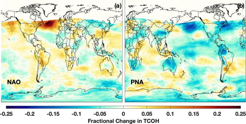
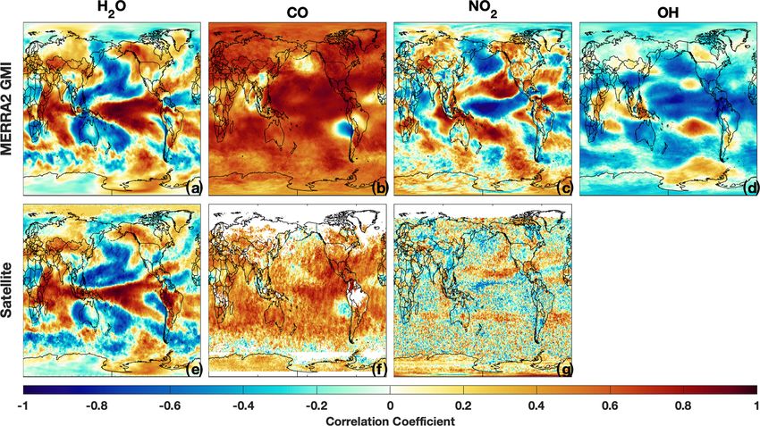
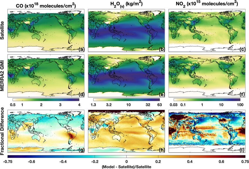
6486                                        D. C. Anderson et al.: Spatial and temporal variability in the hydroxyl radical

ployments. We omit the biomass-burning-influenced parcels         ability discussed in Sects. 4 and 5 are centered in the remote
because small differences in measured and modeled winds           atmosphere.
could result in misplacement of modeled biomass burning
plumes, resulting in unrealistically large differences in OH.     3.2   Evaluation of MERRA-2 GMI with satellite
Inclusion of the biomass-burning-influenced parcels does not            observations
significantly change the model bias but does degrade the cor-
relation. For comparison of the observations to MERRA-2           While there are no remotely sensed observations of tropo-
GMI, hourly data were output by the model and then bilin-         spheric column OH (TCOH), there are satellite observations
early interpolated in the horizontal and linearly interpolated    of OH drivers. Comparing these observations to MERRA-2
in time and in the vertical to the in situ observation time and   GMI allows for model evaluation over larger spatial and tem-
location.                                                         poral scales than with ATom. Satellite data used here include
   MERRA-2 GMI has a OH high bias of approximately                tropospheric CO columns from the Measurement Of Pol-
20 % (Fig. 1a) when compared to observations from ATom            lutants In The Troposphere (MOPITT) instrument, H2 O(v)
2. A regression of measured and modeled OH shows a mod-           from the Atmospheric Infrared Sounder (AIRS), and tropo-
erate to high correlation in both the Southern Hemisphere         spheric NO2 from the Ozone Monitoring Instrument (OMI).
(SH) and NH, with r 2 values of 0.30 and 0.78, respectively.      AIRS is on the Aqua satellite, with a daily local overpass
Normalized mean biases (NMBs) relative to the observations        time of approximately 13:30 LT (local time; applicable to all
are within measurement uncertainty in both the NH (19 %)          times given herein). We use the monthly averaged, level 3,
and SH (16 %), with nearly identical high biases during the       version 6 standard physical retrieval (Susskind et al., 2014)
summer deployment of ATom 1 (Fig. 1c). The compara-               from 2003 to 2018. For MOPITT CO on the Terra satellite,
tively poorer model performance for OH in the SH is being         we use the level 3, version 008 retrieval that uses both near-
driven by continental outflow from South America and New          and thermal-infrared radiances (Deeter et al., 2019) from
Zealand. When data from these regions are omitted (Fig. 1a;       2001 to 2018. MOPITT has a daily local overpass time of
blue stars), the correlation for the SH increases to 0.63 and     approximately 10:30. Both satellite products have a global
the NMB is 22 %. The limited model output at hourly reso-         horizontal resolution of 1◦ × 1◦ . We also use the OMI NO2
lution does not allow for a determination of the cause of this    version 4, level 3 product (Lamsal et al., 2021) from 2005 to
disagreement in continental outflow regions. In the case of       2018. Data have been regridded to 1◦ × 1◦ horizontal resolu-
South America, however, a known high bias in modeled iso-         tion. OMI is located on the Aura satellite and, as with AIRS,
prene, resulting in extremely low OH over the Amazon, is          has a local overpass time of approximately 13:30.
consistent with the disagreement between the simulation and          For comparison of the satellite retrievals to MERRA-2
observations.                                                     GMI, we use monthly fields of the model variables output
   Agreement between observed and modeled CO shows a              at the satellite overpass time. For CO, where averaging ker-
strong hemispheric dependence, with a NMB of −14 % in             nel and a priori information are available for the level 3 MO-
the NH (i.e., the model is lower than observations by 14 %)       PITT data, we convolve the model output with these vari-
and 8 % in the SH during ATom 2, although both hemispheres        ables so that direct comparison between satellite and model
have a strong correlation (r 2 > 0.7). While agreement in the     are possible. While shape factors and scattering weights for
SH improves in ATom 1, with a NMB of 2 % (Fig. 1d), the           the OMI NO2 retrieval are unavailable for the level 3 data,
model underestimate in the NH is even more pronounced             shape factors for the OMI NO2 retrieval are determined from
(NMB = −20 %). This NH low bias in CO is a well-known             a similar setup of the GEOSCCM model, also employing the
problem in global chemistry models (e.g., Naik et al., 2013;      GMI chemical mechanism and MERRA-2 meteorology. Ap-
Stein et al., 2014; Travis et al., 2020) and could be a con-      plying the satellite shape factors to the simulation discussed
tributing factor in the overestimate in OH, as CO is the dom-     here would therefore not result in significant changes in the
inant global OH sink.                                             modeled NO2 . Finally, for AIRS H2 O(v) , averaging kernel in-
   Comparison of the MERRA-2 GMI simulation to in situ            formation was unavailable for the level 3 data, so numerical
observations demonstrates that the model captures the spatial     comparisons between satellite and model should be regarded
variability of OH and its predominant global sink, CO, in the     as more qualitative than quantitative.
remote atmosphere during both the NH summer and winter,              When compared to MOPITT in boreal winter (i.e.,
with the exception of OH off the coast of South America and       DJF – December–February), tropospheric column CO from
New Zealand. The poorer agreement between measured and            MERRA-2 GMI (Fig. 2; first column) shows similar results
modeled OH in regions of fresh, continental outflow suggests      to that found through comparison to the in situ observations,
that modeled relationships between climate modes and OH           namely a low bias in the NH (9 %) and high bias in the SH
in these regions might be more uncertain than in the remote       (7 %). Differences over the tropical Pacific, an area that will
atmosphere. This lack of agreement does not significantly af-     be shown later to have a strong relationship between ENSO
fect the results discussed in this work, as the majority of the   and OH, are generally less than 10 %, while a noticeable high
relationships found between OH and modes of climate vari-         bias exists over parts of South America. Results for June–

Atmos. Chem. Phys., 21, 6481–6508, 2021                                            https://doi.org/10.5194/acp-21-6481-2021
D. C. Anderson et al.: Spatial and temporal variability in the hydroxyl radical                                                    6487

Figure 1. Regression of observed OH (a, c) and CO (b, d) from ATom 2 (boreal winter 2017; a, b) and ATom 1 (boreal summer 2016; c,
d) against hourly output from MERRA-2 GMI interpolated to the ATom flight track. Data from the Southern (blue circles) and Northern
(orange triangles) hemispheres are shown, along with the r 2 , bias, and normalized mean bias (NMB) for each hemisphere. Observations and
model output have been filtered for biomass burning influence. Observations of continental outflow from New Zealand and South America
from ATom 2 are indicated by blue stars.

August (JJA) are spatially similar (Fig. 3), with a NH low             fer. The simulation shows a significant high bias over central
bias of 20 % and overestimates of column CO, averaging                 Africa and the equatorial Atlantic of the order of 100 %, sug-
45 %, in the SH. These areas of high bias over South Amer-             gesting that biomass burning emissions of NOx , the dominant
ica likely result from the high bias in isoprene emissions, as         NO source in this region, are too high. In contrast, concen-
discussed in Sect. 2.2, that would lead to unrealistically high        trations over eastern Asia are too low in the model, suggest-
in situ production of CO.                                              ing errors in the anthropogenic emissions inventory and/or in
   MERRA-2 GMI captures the spatial distribution of                    the NOx lifetime. Strode et al. (2019) also evaluated NO2 in
H2 O(v) , although the model is biased high in both the col-           MERRA-2 GMI, comparing trends in tropospheric column
umn and throughout much of the troposphere. Overestimates              NO2 over the eastern US and eastern China in MERRA-2
in column H2 O(v) are ∼ 14 % in both DJF (Fig. 2h) and                 GMI and OMI. They found that, although trends were simi-
JJA (Fig. 3). These overestimates extend over most of the              lar between the simulation and observations in both regions,
world’s oceans, and only small regions over northern India,            the magnitude of the trends differed, likely due to errors in
central Africa, eastern Russia, and eastern Canada show any            the MACCity emissions inventory.
underestimate in H2 O(v) . Fractional differences in H2 O(v)              As with the in situ observations, comparison between
between MERRA-2 GMI and the different AIRS pressure                    MERRA-2 GMI and satellite retrievals demonstrates that the
levels are most pronounced in the tropical UT (Fig. 4). At             simulation is able to capture the distribution of the chemi-
pressures greater than 700 hPa, modeled H2 O(v) is generally           cal drivers of OH in remote regions which tend to exhibit
within 10 % of the observations, while for pressures less than         the strongest relationship between OH and climate modes
500 hPa, modeled H2 O(v) in the equatorial region disagrees            (see Sect. 4). These results lend confidence to the analysis
with observations by 55 % on average.                                  described in Sects. 4 and 5 and suggest that the findings
   Agreement between observed and modeled NO2 is weaker                in remote regions are likely applicable to the actual atmo-
than for the other species examined here. While MERRA-2                sphere. The large disagreement between the simulation and
GMI appears to capture the regions with local NO2 maxima –             observed column CO and NO2 in regions that are signifi-
notably those over central Africa, eastern China, and the              cantly impacted by biomass burning and/or biogenic emis-
northeastern United States – the magnitudes frequently dif-            sions suggests, however, that modeled relationships of chem-

https://doi.org/10.5194/acp-21-6481-2021                                                 Atmos. Chem. Phys., 21, 6481–6508, 2021
6488 D. C. Anderson et al.: Spatial and temporal variability in the hydroxyl radical
Figure 2. Tropospheric column CO (a, d, g), H2 O(v) (b, e, h), and NO2 (c, f, i) from MOPITT, AIRS, and OMI, respectively (a–c), and
MERRA-2 GMI (d–f) for DJF (December–February). For the satellite retrievals and model, data are averaged over the time range described
in the text for each instrument. The fractional difference between MERRA-2 GMI and the satellite is shown in (g–i).
ical species with modes of climate variability in these re- mass), while the IOD, consistent with its seasonal variability,
gions should be viewed with caution. We further evaluate the only has a widespread correlation with TCOH during SON
ability of the simulation to capture the relationship between (September–November). Similar patterns are found for the
ENSO and CO, H2 O(v) , and NO2 using satellite observations individual layers (Fig. S2 in the Supplement).
in Sect. 5.1.2. Below, we examine the relationships between tropospheric
OH and the various modes of climate variability demon-
strated in Fig. 5. First, in Sect. 5, we show that El Niño events
4 The relationship between simulated OH variability lead to global reductions in tropospheric OH, with changes
and climate modes being driven by decreased secondary production in the UFT
that more than compensates for increased primary produc-
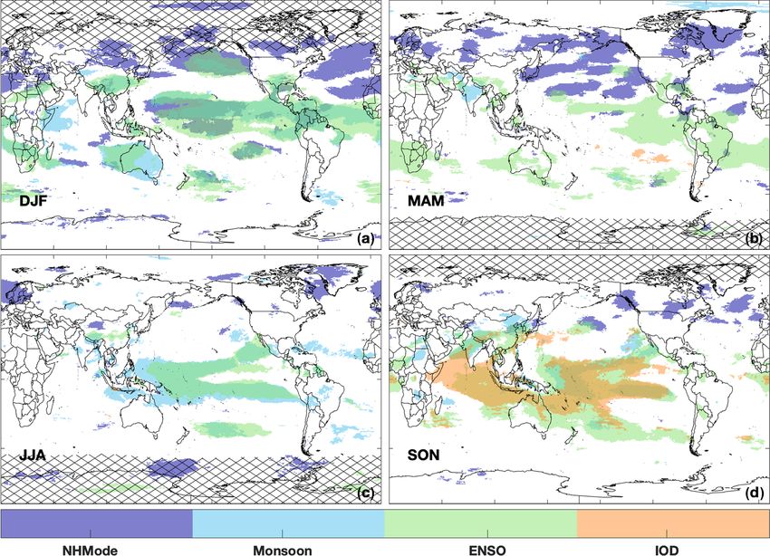
When considered in concert, the modes of climate variability tion in the PBL. In Sect. 6, we demonstrate that the effects
evaluated here (i.e., ENSO, the IOD, and NH modes), along on OH from NH modes of variability, the IOD, and some
with monsoons, explain a substantial fraction of the sim- monsoons have limited spatial scales, as compared to ENSO,
ulated tropospheric OH interannual variability over 19 %– but can significantly alter local OH distributions. In both sec-
40 % of the global troposphere by mass, depending on sea- tions, we also compare simulations from MERRA-2 GMI to
son. Figure 5 highlights regions that show significant correla- simulations from the CCMI, demonstrating that the relation-
tion between TCOH and the NH modes (purple), monsoons ship between OH and climate modes is robust among multi-
(light blue), ENSO (green), and the IOD (orange) for each ple models.
season in MERRA-2 GMI output. In all seasons, correla-
tion with ENSO has the largest spatial extent, but in DJF and
MAM (March–May), for example, the eight NH modes can 5 Relationship between simulated OH variability and
explain TCOH variability over large swaths of the NH, com- ENSO in MERRA-2 GMI
prising 10 % of global, tropospheric mass. In JJA, the com-
bination of the different climate modes and monsoons has To understand the relationship between OH, its drivers, and
the smallest spatial coverage (19 % of the global tropospheric ENSO, we first investigate the OH production rate. In the
Atmos. Chem. Phys., 21, 6481–6508, 2021 https://doi.org/10.5194/acp-21-6481-2021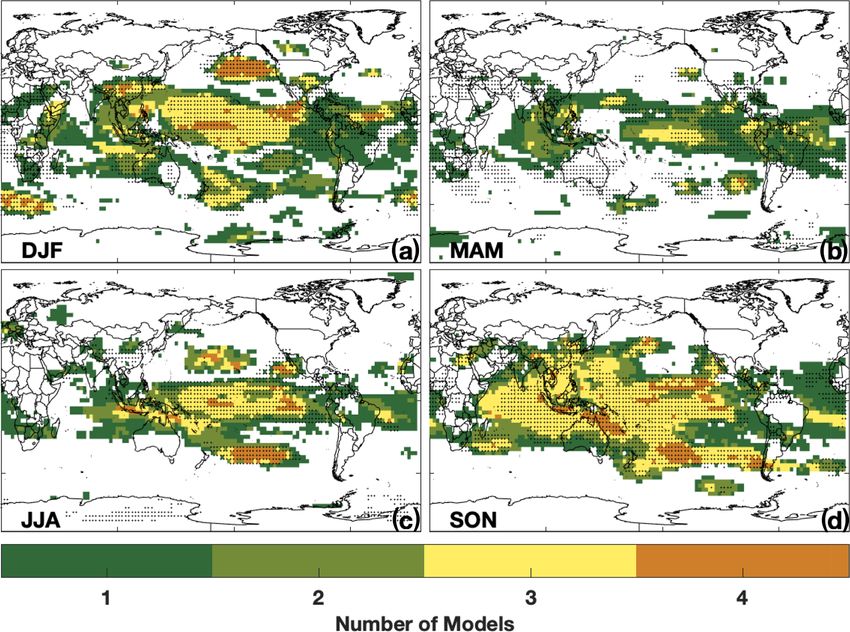
D. C. Anderson et al.: Spatial and temporal variability in the hydroxyl radical                                             6489

Figure 3. Same as Fig. 2 except for JJA (June–August).

                                                                    (e.g., South America and central Africa) do other reactions
                                                                    contribute more than 15 % of the total OH production in the
                                                                    PBL. As will be shown, the effects of ENSO on OH are pri-
                                                                    marily focused away from these regions, so we restrict our
                                                                    analysis to the reactions (R1)–(R4).
                                                                    H2 O2 + hυ → 2OH                                         (R1)
                                                                    NO + HO2 → NO2 + OH                                      (R2)
                                                                    O3 + HO2 → 2O2 + OH                                      (R3)
                                                                    H2 O + O1 D → 2OH.                                       (R4)

                                                                       During El Niño events, the dominance of these individual
                                                                    reactions in producing OH varies with altitude. We focus our
                                                                    analysis on DJF throughout Sect. 5 because that is the season
                                                                    with the largest impact of ENSO on OH, as shown in Fig. 5.
Figure 4. The fractional difference in zonal mean H2 O(v) between   Figure 6 shows the zonal mean of the fraction of total OH
MERRA-2 GMI and AIRS for the different AIRS pressure layers
                                                                    production from the H2 O + O1 D (Fig. 6a) and NO + HO2
for DJF. Positive numbers indicate a high bias in the model.
                                                                    (Fig. 6b) reactions as well as the total OH production rate
                                                                    (Fig. 6c) during El Niño events in DJF. While the production
                                                                    rates along these pathways vary with the ENSO phase, as
MERRA-2 GMI simulation, the OH production rate is pri-              discussed in Sects. 5.2 and 5.3, the relative importance of
marily dependent on Reactions 1–4, where O1 D is produced           the individual reactions is similar during neutral and La Niña
from the photolysis of tropospheric O3 . In the free tropo-         events (not shown) and is in agreement with previous model
sphere, these four reactions comprise at least 95 % of OH           studies (e.g., Spivakovsky et al., 2000).
production in the tropics, on average, and at least 90 % in            The H2 O + O1 D reaction is dominant from the surface to
the PBL. Only in the regions with large biogenic emissions          about 800 hPa through much of the SH and the tropics, while,

https://doi.org/10.5194/acp-21-6481-2021                                            Atmos. Chem. Phys., 21, 6481–6508, 2021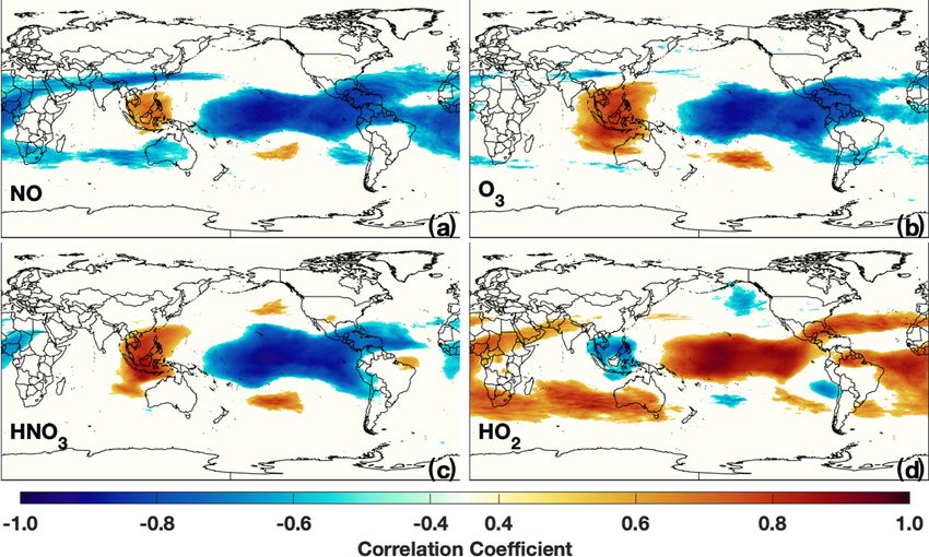
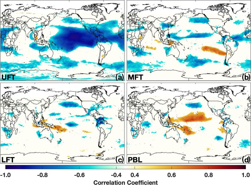
6490                                          D. C. Anderson et al.: Spatial and temporal variability in the hydroxyl radical

Figure 5. Regions that show a significant correlation (absolute value of r > 0.5) between a NH mode (purple), monsoon (light blue), ENSO
(green), or IOD (orange) and TCOH for each season in the MERRA-2 GMI simulation. Regions with TCOH less than 1 × 10¹¹ molec. cm−2
have been hatched out.

Figure 6. Zonal mean of the fractional contribution of the O1 D + H2 O (a) and NO + HO2 (b) reactions to the total OH production rate and
the total OH production rate (c) for El Niño events (MEI > 0.5) for DJF, averaged over 1980–2018.

near the surface, the NO + HO2 reaction only has large im-             ysis reactions generally contribute between 10 % and 30 % of
pacts in the NH midlatitudes. This influence of NOx in the             the total rate (Fig. S3). The dominant OH sink throughout the
NH midlatitudes extends through much of the troposphere. In            troposphere is CO, which is responsible for a 50 % or greater
the UFT, this reaction is the greatest contributor to total OH         OH loss at all tropospheric pressures and latitudes (Fig. S4 in
production at all latitudes except the NH polar region, where          the Supplement) during El Niño events. Because of the dif-
the HO2 + O3 reaction dominates during polar night (Fig. S3            fering importance of the individual OH production reactions
in the Supplement). Total OH production in the polar regions,          with altitude, we first examine the relationship between OH
however, is orders of magnitude lower than in the tropics.             and ENSO for TCOH (Sect. 5.1) and then separately for the
Outside of the polar regions, the HO2 + O3 and H2 O2 photol-           PBL (Sect. 5.2) and the UFT (Sect. 5.3). Finally, in Sect. 5.4,

Atmos. Chem. Phys., 21, 6481–6508, 2021                                                  https://doi.org/10.5194/acp-21-6481-2021
D. C. Anderson et al.: Spatial and temporal variability in the hydroxyl radical                                             6491

we investigate the MFT and LFT, where the effects of ENSO          sons are similar to the composite figures showing OH anoma-
on OH are more limited.                                            lies during El Niño (Fig. S5 in the Supplement). For MAM,
                                                                   the EOF again shows regions with a negative sign over much
5.1     Tropospheric column OH                                     of the Northern Hemisphere, with the largest magnitude cen-
                                                                   tered over the Pacific Ocean, India, and the Atlantic coast
5.1.1    The relationship between simulated TCOH and               of the United States. Regions with an opposite sign include
         ENSO                                                      the Maritime Continent and much of central Africa. In SON,
                                                                   almost all of the tropics show some response, with major
As shown in Fig. 7, TCOH decreases by 3.3 % during                 centers off the east coast of Papua New Guinea and off the
El Niño events (relative to neutral events) equatorward of         west coast of Sumatra. In addition, there is a larger response
30◦ in DJF and is characterized by widespread decreases in         over the Indian Ocean than for other months, also evident in
the tropics and subtropics, especially in northern Australia       the regression of TCOH with the MEI, suggesting the pos-
and west–central and southern Africa. Regional increases are       sible influence of the IOD, which is correlated with ENSO
found over eastern Africa, the east–central Pacific, south-        (r 2 = 0.30). This seasonal component in the strength of the
ern South America, and Indonesia. Maximum decreases in             relationship between the EOF and the MEI is also reflected
TCOH are of the order of 4.5 × 10¹¹ molec. cm−2 (∼ 10 %–           in the correlation analysis (Fig. 5), where the area of corre-
15 %) and are centered over northern Australia, while max-         lation between TCOH and the MEI maximizes in DJF and
imum increases in TCOH (∼ 2.5 × 10¹¹ molec. cm−2 ) are             minimizes in JJA.
centered over Sumatra.
    During La Niña events, TCOH increases relative to neu-         5.1.2   The relationship between TCOH drivers and
tral events over much of the globe, although the changes are               ENSO
not necessarily symmetric with those seen during El Niño
events. Increases over Australia are of the order of 1 to          To understand the factors driving ENSO-related changes
2 × 10¹¹ molec. cm−2 , on par with the decreases seen during       in TCOH, we also investigate the relationship between
El Niño, but the changes during La Niña are centered over          OH precursors and ENSO. Figure 6 demonstrates that the
western Australia and the Indian Ocean. Over the Pacific,          O1 D + H2 O and NO + HO2 reactions control zonal mean
the magnitude of the OH increase is lower (of the order of         OH production in the tropics. As a result, we investigate
0.5 to 1 × 10¹¹ molec. cm−2 ) than the decreases found during      the relationship between the tropospheric column H2 O(v) ,
El Niño, and some regions off the coast of Hawaii and Papua        CO, NO2 , and ENSO using both MERRA-2 GMI output
New Guinea show decreases during both ENSO phases. Be-             and satellite retrievals. We use NO2 here, instead of NO,
sides these two regions, there are also significant decreases in   because of its observability from space, although simulated
OH over eastern Africa and in the southern portion of South        NO demonstrates similar spatial correlation patterns with the
America.                                                           MEI as simulated NO2 .
    Consistent with these widespread changes in TCOH, EOF             Regression of total column H2 O(v) from AIRS against the
analysis demonstrates that, over most seasons, with JJA be-        MEI (Fig. 9e) reveals a tripole pattern over the Pacific Ocean,
ing the notable exception, ENSO is the dominant mode of            with an area of positive correlation throughout much of the
OH variability. Figure 8 shows the spatial component of the        equatorial Pacific Ocean and areas of anti-correlation pole-
first EOF of TCOH for the four seasons. While EOF analysis         ward of this region, in agreement with previous work (e.g.,
does not quantify changes in column content, it does high-         Shi et al., 2018). Each of these areas is well captured by the
light, for each mode of variability, regions where changes in      MERRA-2 GMI simulation (Fig. 9a), showing nearly iden-
TCOH are most prominent. For DJF, the first EOF (Fig. 8a) is       tical spatial patterns and strength of correlation over most
almost identical to the composite figure showing OH anoma-         of the globe. This relationship between H2 O(v) and ENSO
lies during El Niño (Fig. 7a). Likewise, the temporal com-         can be explained by the increased convective uplifting in the
ponent of the first EOF strongly correlates with the MEI           equatorial Pacific and the associated increased subsidence
(r 2 = 0.70; Table 2). In DJF, the first EOF is responsible for    poleward of this region during El Niño events. While the
29 % of the total spatial variance for TCOH. Although ENSO         anticorrelation between H2 O(v) and the MEI over Australia
is the dominant mode, however, 70 % of the spatial variance        and southern Africa is consistent with the decrease in TCOH
is still unexplained. In JJA, ENSO influence on OH is much         over these regions during El Niño events (Fig. 7), the positive
weaker, with a correlation between the first EOF and TCOH          correlation between H2 O(v) and the MEI over the equatorial
of r 2 = 0.25, consistent with the seasonal cycle of ENSO.         Pacific suggests there must be competing effects from other
    While the spatial pattern of the EOF varies seasonally         OH drivers in order to explain the decreases in TCOH in this
(Fig. 8), ENSO shows similar levels of correlation to the tem-     region.
poral component of the first EOF in MAM and SON as for                Simulated tropospheric column NO2 is strongly anti-
DJF, with r 2 values of 0.54 and 0.60, respectively. Likewise,     correlated with ENSO over the equatorial Pacific, indicating
the spatial patterns of the first EOF of TCOH for these sea-       a suppression of OH production when the MEI is positive

https://doi.org/10.5194/acp-21-6481-2021                                            Atmos. Chem. Phys., 21, 6481–6508, 2021
6492 D. C. Anderson et al.: Spatial and temporal variability in the hydroxyl radical
Figure 7. Absolute difference in TCOH between El Niño events and neutral events (a) for DJF, averaged over 1980–2018. El Niño and neutral
events are defined as a season having an MEI value greater than 0.5 or an MEI value between −0.5 and 0.5, respectively. The analogous plot
for La Niña events (MEI less than −0.5) is also shown (b). Panel (c) shows the average OH column for neutral events. The 1980–2018 time
period includes 11 El Niños, 12 La Niñas, and 15 neutral events in DJF.
Table 2. For each season, we show the r 2 of the correlation of the temporal component of the EOF that has the highest correlation with the
MEI for TCOH and for OH in each layer. In addition, we also indicate the percent (Pct.) of the total spatial variance explained by that EOF.
With the exception of the values indicated by an asterisk (∗ ), the first EOF has the highest correlation with the MEI. Those indicated with an
asterisk (∗ ) are the second EOF.
Column UFT MFT LFT PBL
Season Pct. variance r2 Pct. variance r2 Pct. variance r2 Pct. variance r2 Pct. variance r2
DJF 29.4 0.7 37.6 0.73 20.8 0.81 11.7∗ 0.55 12∗ 0.85
MAM 25.9 0.54 36.2 0.61 23.4 0.40 9.5∗ 0.48 9.3∗ 0.59
JJA 30.7 0.25 44.6 0.14 29 0.15 27.7 0.06 39.4 0.07
SON 33.2 0.60 41.1 0.50 22.8 0.63 12.3∗ 0.59 9.3∗ 0.63
(El Niño), which is consistent with Fig. 7. Column NO2 ex- ral and spatial averaging, OMI is capable of capturing the
hibits the opposite correlation pattern to that of H2 O(v) over variability in tropospheric NO2 , even in remote regions with
the Pacific, with decreases in NO2 in regions with increased low concentrations.
H2 O(v) and vice versa. The similarities in the spatial corre- Tropospheric column CO and the MEI are positively cor-
lation patterns for NO2 and H2 O(v) with the MEI suggests related over most of the globe in both MERRA-2 GMI and
that convection is also at least partially driving the changes in MOPITT (Figs. 9b and f, respectively), suggesting strong
in NO2 in the equatorial Pacific. Changes in the Walker circu- increases in CO during El Niño events. This increase in CO
lation associated with El Niño events have been shown to re- is associated with increased biomass burning, particularly in
distribute O3 in the tropics, resulting in a dipole pattern over Indonesia, and is consistent with the modeled decrease in OH
the western and central Pacific (Oman et al., 2011). Analy- (e.g., Duncan et al., 2003a) and with the widespread decrease
sis of vertical winds and the NO2 anomaly suggests a similar in TCOH over much of the tropics.
mechanism for NO2 .
Correlations between OMI NO2 and the MEI suggest 5.2 The planetary boundary layer
similar relationships as found in the MERRA-2 GMI sim-
ulation, although the correlations are not as robust as 5.2.1 The relationship between PBL OH and ENSO
for the other satellite variables examined here. This is
In contrast to the tropospheric column (Fig. 7), mean mass-
likely because tropospheric NO2 columns over the ocean
weighted OH (e.g., Lawrence et al., 2001) in the PBL in-
are frequently at or below the instrumental average noise
creases globally by 1 % during El Niño events (Fig. 10),
(5 × 10¹⁴ molec. cm−2 ). As with the simulation, OMI sug-
although regional differences are significantly larger. PBL
gests broad regions of anti-correlation between ENSO and
OH exhibits an area of strong positive correlation with the
NO2 in the equatorial Pacific and the Gulf of Alaska as well
MEI (Fig. 11d) over the central Pacific, marked by increases
as a region of positive correlation in the extra-tropical NH
in concentrations of the order of 2–3 × 10⁵ molec. cm−3 ,
Pacific. These results demonstrate that, with enough tempo-
approximately 15 % higher than concentrations in neutral
Atmos. Chem. Phys., 21, 6481–6508, 2021 https://doi.org/10.5194/acp-21-6481-2021D. C. Anderson et al.: Spatial and temporal variability in the hydroxyl radical 6493 Figure 8. The first EOF of TCOH from MERRA-2 GMI for DJF (a), MAM (b), JJA (c), and SON (d). Figure 9. Regression of tropospheric column H2 O(v) (a), CO (b), NO2 (c), and OH (d) from MERRA-2 GMI (top) and satellite retrievals from AIRS (e), MOPITT (f), and OMI (g) against the MEI for DJF over the satellite lifetime. https://doi.org/10.5194/acp-21-6481-2021 Atmos. Chem. Phys., 21, 6481–6508, 2021
6494                                           D. C. Anderson et al.: Spatial and temporal variability in the hydroxyl radical

Figure 10. Same as panels (a) and (b) of Fig. 7 except for the PBL level.

Figure 11. Correlation of OH from MERRA-2 GMI with the MEI for the different atmospheric layers in DJF.

events. Changes in the PBL during La Niña are smaller, with             DJF and MAM and over Indonesia in SON. In general, the
localized concentration decreases of about 5 %–10 % over                r 2 with ENSO is 0.5 or higher, and the mode contributes ap-
the tropical Pacific (Fig. 10b). Regions with significant cor-          proximately 10 % of the total spatial variance, although cor-
relation between PBL OH and the MEI are distinctly smaller              relation in JJA (r 2 = .07) is negligible.
than in the UFT (Fig. 11) and for TCOH (Fig. 5a), fur-                     In contrast to the ENSO-related EOFs, the first EOF
ther emphasizing the comparatively limited spatial effects of           (Fig. S7 in the Supplement) for the DJF PBL layer reveals
ENSO in the PBL.                                                        a spatial pattern much more limited to continental regions
   The more geographically limited changes in OH, shown                 and areas of continental outflow, suggesting that this mode
by the composite and regression analyses, are consistent with           of variability is potentially reflective of long-term emission
EOF analysis. During all seasons except JJA, ENSO corre-                trends in both anthropogenic and biomass burning emissions.
lates more strongly with the second EOF for the PBL (Ta-                This is more evident in the first EOF for JJA, where the spa-
ble 2), suggesting another mechanism is the dominant mode               tial pattern shows opposite signs over regions with known net
of variability. The spatial pattern of the second EOF for PBL           emissions reductions (the United States, portions of Europe,
OH varies markedly across seasons (Fig. S6 in the Supple-               and Japan) and those with known net emissions increases
ment), with the largest signal over the tropical Pacific during

Atmos. Chem. Phys., 21, 6481–6508, 2021                                                  https://doi.org/10.5194/acp-21-6481-2021
D. C. Anderson et al.: Spatial and temporal variability in the hydroxyl radical                                                  6495

Figure 12. Correlations of the MEI with the production rate of OH from the H2 O + O1 D reaction (a) for DJF and the total OH production
rate, as defined in the text, (b) for the PBL level are shown.

Figure 13. Correlation of the indicated species with the MEI for the PBL level for DJF.

(China, India, and the Middle East) over the 1980–2018 pe-              MEI demonstrates that changes in this reaction are driving
riod examined here.                                                     changes in OH in the tropics during El Niño events.
                                                                           To understand the relationship between the OH produc-
5.2.2   The relationship between PBL OH drivers and                     tion rate and ENSO in the PBL, we examine the changes in
        ENSO                                                            H2 O(v) and O1 D (Fig. 13). The spatial correlation of H2 O(v)
                                                                        and the MEI in the PBL exhibits a tripole pattern similar to
Approximately 80 % of the zonal mean OH production in the               that seen in the tropospheric column (Fig. 9a). While H2 O(v)
tropical PBL during El Niño events is from the H2 O + O1 D              is correlated with the MEI in the equatorial Pacific, which
reaction (Fig. 6a). Figure 12 shows the correlation of the              would lead to increases in OH production, H2 O(v) is anti-
MEI against both OH production from this reaction and                   correlated with the MEI near the Hawaiian Islands and in the
the total OH production rate for the PBL. Similar plots for             south Pacific, which would lead to decreased OH production
the other OH production reactions are shown in Fig. S8                  in these regions. Because OH increases in these areas during
in the Supplement. The nearly identical regression pattern              El Niño events, the decreased H2 O(v) is offset by increases
for the H2 O + O1 D and the total production rate with the

https://doi.org/10.5194/acp-21-6481-2021                                                  Atmos. Chem. Phys., 21, 6481–6508, 2021
You can also read