Stepwise slime mould growth as a template for urban design
←
→
Page content transcription
If your browser does not render page correctly, please read the page content below
www.nature.com/scientificreports
OPEN Stepwise slime mould growth
as a template for urban design
Raphael Kay1,2*, Anthony Mattacchione3, Charlie Katrycz2 & Benjamin D. Hatton2*
The true slime mould, Physarum polycephalum, develops as a vascular network of protoplasm,
connecting node-like sources of food in an effort to solve multi-objective transport problems. The
organism first establishes a dense and continuous mesh, reinforcing optimal pathways over time
through constructive feedbacks of protoplasmic streaming. Resolved vascular morphologies are
the result of an evolutionarily-refined mechanism of computation, which can serve as a versatile
biological model for network design at the urban scale. Existing digital Physarum models typically use
positive reinforcement mechanisms to capture meshing and refinement behaviours simultaneously.
While these automations generate accurate descriptions of sensory and constructive feedback, they
limit stepwise design control, reducing flexibility and applicability. A model that decouples the two
“phases” of Physarum behaviour would enable multistage control over network growth. Here we
introduce such a system, first by producing a site-responsive mesh from a population of nutrient-
attracted agents, and then by independently calculating from it a flexible, proximity-defined shortest-
walk to produce a final network. We develop and map networks within existing urban environments
that perform similarly to those biologically grown, establishing a versatile tool for bio-inspired urban
network design.
The true slime mould, Physarum polycephalum, is a single-celled amoeboid organism with a remarkable aptitude
for design (Fig. 1). The slime mould cell grows (1 mm/h to 1 cm/h) as a tubular network of protoplasm, guided
by the nutrient-rich environment within which it forages (Fig. 2a, t = 5 days)1. As Physarum encounters discrete
food sources along its path, it develops from a preliminary mesh into a refined network, comprising both direct
and indirect pathways between sources of nutrition (Fig. 2a, t = 7 days, Supplementary Fig. S1)2. Such a network
is a remarkable accomplishment: while many biological organisms have established sophisticated neural circuitry
to process, learn from, and adapt to sensory information, the slime mould has instead relied on a decentralized
and fluidic form of adaptive physical computing3,4. The tubular and gel-like cytoskeleton of the organism acts as
a spatially-varied molecular motor5, comprising many distinct oscillator units distributed across the cell. Each
unit generates a wave-like contraction at a frequency dependent on both the neighbouring contraction frequency
and the presence of attractants (e.g., food) and repellants (e.g., light) within its immediate environment5–11.
Attractants (e.g., food) cause molecular receptor binding at the surface membrane of the o rganism6. This leads
to an increase in the contraction frequency of the units nearest to the attractant, shuttling cytoplasmic fluids
towards nutrient-rich regions12. Molecular binding also causes a local decrease in surface tension at the point
of attraction, inducing a hydrostatic pressure difference, forcing cytoplasmic fluid to additionally flow towards
nutrition6. Cell morphology is dictated by feedback loops of collective oscillation and cytoplasmic fluid flows,
whereby the organism can simultaneously refine efficient links and starve and destroy r edundancies13.
This reactive routing mechanism enables highly sophisticated behaviour: Physarum is able to navigate mazes
with a minimum path length14–16, form proportional contacts between unique food sources for an optimal diet17,
grow as a mathematical minimum tree18, remember where it has been7, anticipate regular events19, and even
mimic with impressive accuracy the Tokyo rail system20 and Autobahn21. This non-neural, fluidic, biological
computer—able to process new information, make informed decisions, and learn without the aid of a neural
circuit—represents an intriguing computational model for unconventional data processing, problem solving,
and memory storage22. Efforts to study and capture this capacity have been established, whereby Physarum gates
have been leveraged to perform logical operations23, while Physarum cells have been explored as tactile, chemical,
and colour s ensors24–26, as well as processing c hips27.
1
Department of Mechanical and Industrial Engineering, University of Toronto, Toronto, Canada. 2Department
of Materials Science and Engineering, University of Toronto, Toronto, Canada. 3John H. Daniels Faculty
of Architecture, Landscape, and Design, University of Toronto, Toronto, Canada. *email: raphael.kay@
mail.utoronto.ca; benjamin.hatton@mail.utoronto.ca
Scientific Reports | (2022) 12:1322 | https://doi.org/10.1038/s41598-022-05439-w 1
Vol.:(0123456789)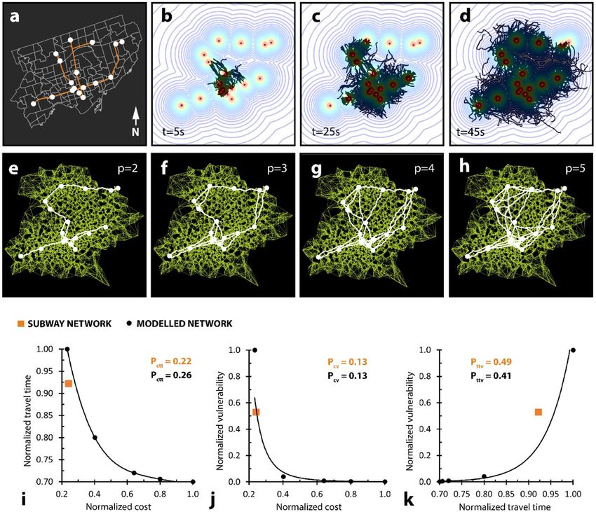
www.nature.com/scientificreports/
Figure 1. Intelligent growth network formation by the active plasmodial Physarum polycephalum. (a–l) Digital
photographs and (m–o) optical microscope images of various stages of slime mould growth using oat flakes as
nutrient sources. All images (other than l) photographed after 4 days of growth. (l) Photographed after seven
days of growth.
Physarum for urban design
Slime mould can also crucially serve as a biological model for adaptive computational network d esign20. Phys-
arum, like colonies of microorganisms28,29, fungal networks30, and wood-ant trails31, represents a highly-efficient
and decentralized growth network. The biological principles that underpin the organization of this system have
undergone thousands of cycles of evolution, and can provide fundamental insights for dealing with complex
networking problems of our own (e.g., road p lanning21,32, railway p
lanning20, wireless sensor r outing33), and
particularly at the scale of the city. Urban design—simplified here as the formal conceptualization of urban
networks (e.g., roadways and railways)—has historically occurred without well-understood or well-defined
criteria20,34. Major arterial Paris roadways, for instance, were famously introduced in the mid-1800s on the basis
of modernization and circulation35,36. While grid-like urban morphologies were developed in Barcelona, driven
in large part by political forces like land-ownership37. Ebenezer Howard’s Garden City was conceptualized as a
utopian revolution against industrialized urban f orm38. Yet, around the same time, Le Corbusier conceptualized
the motorway networks of Pessac, France to oppositely prioritize automobile and ‘industrial’ e fficiency39, which
is a trend that has continued in the planning of many modern city networks in the United S tates40.
In the 1960s, architects at the Institute for Lightweight Structures in Stuttgart began experimenting with
self-assembling natural materials, hoping to find generalizable physically-optimized solutions for urban network
design. Frei Otto, who pioneered theories of material computation in design, used soap films to connect a set
of points as a minimal surface, generating what can be extrapolated as a minimal-spanning network (or Steiner
Tree) for given urban geometries41,42. This work has inspired a series of computational explorations since41–44,
focusing primarily on digital computation of urban networks.
Physarum, as a biological computer, has also been tasked with similar urban design problems. Slime moulds
have ‘redesigned’ Iberian roadways45, establishing transport networks that differ from existing road segments, but
that maintain comparable transport performance. Similarly, Physarum has ‘rerouted’ the M6 motorway through
Newcastle32, and provoked questions regarding the redundancy of the Mexican highway system46. Indeed, while
the organism can impressively reconstruct existing anthropically-designed urban n etworks20, the very discrepan-
cies between city infrastructures, and their biologically-grown Physarum analogues, have proven equally crucial
for understanding characteristics of both urban network planning and Physarum intelligence20,21,32,46.
Physarum modelling
Models, developed in order to both understand and mimic the organism’s behaviour, have emphasized aspects
of attractor-based foraging47, environment-driven morphology1, and flux-induced cytoplasmic streaming (i.e.,
flow)20,48,49. For example, Wu et al. developed networks by modelling cellular foraging along the gradient of nutri-
ent attractors and anti-attractors47. Spanning trees grew serially, as a growth point moved along a nutrient-poor
terrain under the influence of a field source. In another model, two agent-like Physarum populations searched
across a nutrient-populated domain, sampling for chemo-nutrients and existing trails (i.e., regions where the cell
had already occupied)50. Distinct behaviours, dictating agent movement, reproduction, and elimination, enabled
Scientific Reports | (2022) 12:1322 | https://doi.org/10.1038/s41598-022-05439-w 2
Vol:.(1234567890)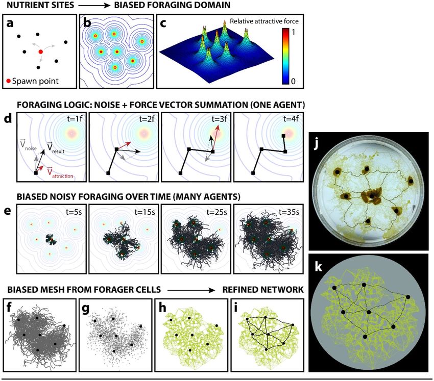
www.nature.com/scientificreports/
Figure 2. Simplified principles of plasmodial Physarum polycephalum growth. (a) Growth of the plasmodium
across seven-day observation period. (b) Illustrated depiction of plasmodial growth according to food source
proximity. This behaviour leads to mesh clustering (phase one). (c) Illustrated depiction of mesh clustering, with
mesh regions illustrated. (d) Illustrated depiction of network refinement and shortest-path optimization (phase
two), where only a refined network remains and is illustrated. Illustrations overlaid atop true photographs.
a converging network that solved mazes and found the shortest path between nodes. Tero et al. established a Phys-
arum model that leveraged feedback loops between network thickness and protoplasmic flux20. Greater streaming
between two food sources induced thickening of the connecting network edge. Networks started as randomly
meshed lattices, sidestepping initial foraging behaviour, but still evolved to solve transportation problems.
Some flux-based, cellular automatons were established that introduced membrane condition changes and
amoebic motion as a basis for network a daptation14,51. These models leveraged changes in the “hardness” or
“softness” of the cell, analogous to ectoplasmic repolymerization, to establish rules for cytoplasmic flow and
morphogenesis, approximating a Steiner-tree and solving a maze. Jones developed both passive52 and a ctive53
particle-based models for Physarum growth. Passive populations refer to those with agents that only respond
to their environment, while active populations comprise agents that can also modify their environment. These
models captured aspects of both initial network formation (meshing), and adaptive network refinement. Parti-
cles moved to approximate nuclei subdivisions throughout Physarum growth. Particle resistance was associated
with particle density, determined through physical and sensory particle interactions. Following initialization,
particles secreted a diffusing chemoattractant, attractive to the nearby particles. This generated a feedback of path
reinforcement, as nearby particles were more likely to travel along, and further amplify, well-established trails.
Physarum network morphology has also been compared with the Toussaint hierarchy of proximity graphs54,55.
This hierarchy describes a series of graphs that increase in connectivity, beginning with a minimum spanning
tree, where each proceeding graph contains the edges of the former. It has been speculated that Physarum grows
in stages that mimic successive graphs within the Toussaint h ierarchy54. Plasmodium sites have been abstracted
as a set of points, growing into a nearest-neighbourhood graph, minimum spanning tree, relative neighbour-
hood graph, Gabriel graph, and finally into a Delaunay t riangulation54,56. Proximity graphs have also been used
to systematically compare Physarum networks with urban transport networks: the intersection of a Gabriel graph
and Physarum ‘graph’ grown between oats representing major Mexican cities was shown to be nearly identical
to the intersection of a Gabriel graph and the Mexican motorway graph i tself46.
In this work, we are concerned with two simplified principles of Physarum growth. The first: Physarum for-
ages under the influence of attractants across its foraging domain, and establishes a highly granular mesh biased
to this attractor field (Fig. 2b,c). The second: Physarum refines this granular mesh, establishing from it a simpler
network that solves a multi-objective transportation problem (Fig. 2d). This robust biological network balances
cost (i.e., total length of all network edges), travel time (i.e., average edge length required to connect two points
Scientific Reports | (2022) 12:1322 | https://doi.org/10.1038/s41598-022-05439-w 3
Vol.:(0123456789)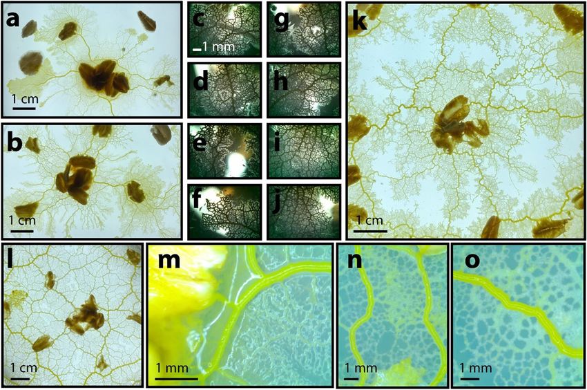
www.nature.com/scientificreports/
Figure 3. Modelled Physarum growth logic. (a) Plot showing seven reference food sources. (b) Contour plot of
the force field generated from (a). (c) Surface topography showing relative attraction force intensity of (b). (d)
Illustrated foraging logic for a single agent. At each frame, the noise vector is summed with the attraction vector,
generated as a function of proximity to food source. (e) Screen captures of agent-based model growth over time
until all food sources have been colonized. (f) Final agent path geometry, from t = 35 s. (g) Point cloud from
paths in (f). (h) Mesh generated from points in (g). (i) Shortest-walk calculation to produce refined network
from mesh in (h). (j–k) Biological versus modelled mesh growth with overlaid network for equivalent reference
food sources.
within a network), and vulnerability (i.e., increase in travel time for the removal of an average segment (i.e., fault)
within a network). These constraints are equally ubiquitous in engineered networks across several length-scales.
While some models have considered either foraging and refinement principles exclusively20,47, the vast
majority have integrated these behavioural elements dependently, cleverly establishing path-reinforcement feed-
backs that simulate the sensory, construction, and adaptive refinement behaviours of the biological organism
simultaneously14,50,53. These systems serve as an exceptional basis for understanding and replicating the feedback
mechanism of the Physarum cell. However, their intrinsic growth-rule dependencies may also limit external
design control and application. A model that describes initial construction independently from network refine-
ment enables compartmentalized system design, which may be particularly beneficial where network refinement
constraints are strict (e.g., urban infrastructure). In such a decoupled model, the network refinement process,
specifically concerned with balancing the final transport system cost, travel time, and vulnerability to fault, is
independent of the preliminary meshing process, introducing stepwise control over network evolution. We
hypothesize that by describing construction and refinement behaviours independently, while the constructive
feedback mechanism of the organism is sidestepped, a more versatile and accessible network design tool can
be established. The objective of this work is to develop and demonstrate this design tool for urban networks.
Here we report a model that captures, in two discrete steps, the meshing and refining behaviour of the motile
Physarum cell. We first developed an agent-based simulation to generate a mesh (i.e., proximity graph) uniquely
responsive to a given set of food sources (Fig. 3a–h). We next calculated a modified shortest walk between all
such sources along this mesh to establish a refined network (Fig. 3i). We demonstrated adaptive control over total
walk length (i.e., network cost), travel time, and fault vulnerability (Fig. 4). We demonstrated nearly identical
Scientific Reports | (2022) 12:1322 | https://doi.org/10.1038/s41598-022-05439-w 4
Vol:.(1234567890)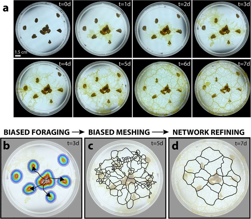
www.nature.com/scientificreports/

                                  Figure 4.  Tunable modelled network behaviour. (a–d) Different shortest-walk calculations for the same mesh,
                                  but with unique proximity coefficient values. (e) Plot relating network cost, normalized to the largest cost, to
                                  proximity coefficient. Trendline is a linear function. (f) Plot relating network travel time, normalized to the
                                  largest travel time, to proximity coefficient. Trendline is a third-order polynomial function. (g) Plot relating
                                  network vulnerability, normalized to the largest travel vulnerability, to proximity coefficient. Trendline is a
                                  power function.

                                  network performance (cost, travel time, fault vulnerability) between our modelled and grown Physarum net-
                                  works (Fig. 5c–e), and we demonstrated varied modelled network performance when compared with existing
                                  urban networks (Figs. 6i–k, 7i–k, respectively). Finally, using these techniques that leverage attractor-biased
                                  agent propagation, we established urban networks using unconventional sets of attractors—in particular, nodes
                                  representative of urban population density (Supplementary Fig. 8a–d).

                                  Results
                                  Two‑stage growth characterization. We observed the vegetative state (plasmodium) of the common
                                  slime mould Physarum across a 14-day period (Figs. 1, 2a). We arranged a collection of oats on otherwise nutri-
                                  ent-poor agar plates and placed a small sample of the active plasmodium in the center of each plate. Within
                                  the first few days, the Physarum established a dense mesh-like lattice, moving towards areas of high nutrient
                                  concentration as it foraged (Fig. 2a, t = 2 days). By the third day, the Physarum cell began refining this mesh, as
                                  it simultaneously continued to expand (Fig. 2a, t = 3 days). Refinement continued into the seventh day (Fig. 2a,
                                  t = 7 days), by which time a resolved network became clearly visible. We established three general principles of
                                  growth to describe the motile Physarum cell: biased foraging, biased meshing, and network refining (Fig. 2b–d).
                                  From these, we developed a model to approximate two independent stages that characterized this behaviour:
                                  biased meshing (which considers biased foraging) (Fig. 3a–h), and network refining (Figs. 3i, 4).

                                  Stage one: biased meshing. We implemented an agent-based model to simulate biased foraging and
                                  meshing, based on a chemoattractant gradient. We developed a series of simple rules to define agent behaviour.
                                  Most fundamentally, the movement of agents was dictated by a summation of two force vectors, one stochastic
                                  and the other deterministic. The deterministic component was based on food attraction within a domain of
                                  foraging. For a given set of attractor points (oats), we established an attractor field within the domain of Phys-
                                  arum foraging. We defined the square of the force exerted by a food source on any given agent to be inversely
                                  proportional to the distance between the agent and food source. Equation (1) describes the relationship between
                                  the magnitude of the force felt on a given agent (Ffood on agent), the distance between that agent and a closest nutri-
                                  ent source (oat flake) (D), and a force constant (c). This force constant, c, can be specified in the model to alter
                                  the noisiness of foraging behaviour. In our experiments, we modelled Physarum with a force constant of 10. For
                                  a set of oats, as digitized from photographs of experimental Physarum growth (Fig. 3a), the relative attractor
                                  field is illustrated in Fig. 3b,c. This field specifies the attraction force felt by an agent given its position within the
                                  domain. Distances between agents and each attractor point were continuously sampled, and the attractive force
                                  of a closest food source was mapped to each agent.

                                                                                     Ffood on agent = c/D.                                                (1)

Scientific Reports |   (2022) 12:1322 |                 https://doi.org/10.1038/s41598-022-05439-w                                                         5

                                                                                                                                                      Vol.:(0123456789)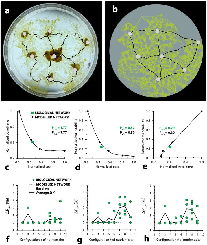
www.nature.com/scientificreports/
Figure 5. Performance of the modelled networks is within 4% of the performance of the biological networks.
(a) Grown Physarum mesh with overlaid network (t = 5 days). (b) Modelled Physarum mesh with overlaid
network. (c) Plot relating network cost to travel time for both grown (green) and modelled (black) networks.
Trendline is a third-order polynomial function. (d) Plot relating network cost to vulnerability for both grown
(green) and modelled (black) networks. Trendline is a third-order polynomial function. (e) Plot relating
network travel time to vulnerability for both grown (green) and modelled (black) networks. Trendline is a linear
function. All performance values normalized to the largest value. Modelled performance values displayed on the
plots represent performance for the closest modelled point to the grown point (green) along the trendline. (f–h)
Performance differences across multiple attractor patterns and growth repeats between biological and modelled
networks are consistently within 4% of one another. Green dots represent grown networks. Smooth black lines
represent average performance differences between all grown and modelled networks at each oat layout, where
difference is taken between the grown network point to the closest point along the modelled network curve. P tt/c
is the network travel time over the network cost; P v/c is the network vulnerability over the network cost; P
v/tt is
the network vulnerability over the network travel time. Plots displayed in c-e represent data from oat layout 7.
Scientific Reports | (2022) 12:1322 | https://doi.org/10.1038/s41598-022-05439-w 6
Vol:.(1234567890)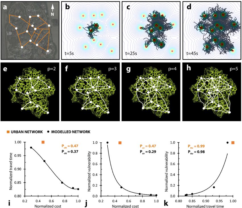
www.nature.com/scientificreports/
Figure 6. Built versus modelled amusement park network performance is varied. (a) Network to describe
Canada’s Wonderland. Background image obtained from Google Maps. (b–d) Modelled growth to establish
mesh to describe Canada’s Wonderland. (e–h) Different shortest-walk calculations for the same mesh, generated
from (d), but with unique proximity coefficient values. (i) Plot relating network cost to travel time for both
built (orange) and modelled (black) networks. Trendline is a third-order polynomial function. (j) Plot relating
network cost to vulnerability for both built (orange) and modelled (black) networks. Trendline is a power
function. (k) Plot relating network travel time to vulnerability for both built (orange) and modelled (black)
networks. Trendline is an exponential function. All performance values normalized to the largest local value.
Modelled performance values displayed on the plots represent performance for the closest modelled point to the
built point (orange) along the trendline.
We initialized modelled Physarum growth by first generating a population of agents, n, where n = 50 for all
experiments, from the center of the substrate domain (Fig. 3d, t = 5 s, and at the spawn point demonstrated in
Fig. 3a). The substrate was defined to be equiaxial, measuring 800 × 800 pixels. Agents foraged at a constant
rate (1.5 pixels per frame). We captured growth at 60 frames per second (agents therefore foraged at 90 pixels
per second). Each frame, we generated the heading component of the stochastic movement vector using a one-
dimensional Perlin noise (number-generating) algorithm. Perlin noise is an algorithm initially developed for
procedural texture generation in computer g raphics57. This algorithm maintains a “memory” of its latest state, and
produces a number that is related to the number generated directly before it. The Perlin noise algorithm gener-
ates numbers within a specified range at a specified time-step, known as the first octave. To produce smoothed
out pseudo-random behaviour, the function sums the set of numbers produced in this first octave with those
produced at all of the smaller octaves, where each subsequent octave doubles the frequency of the timestep and
halves the range. This approach enables a time-dependent number generation, producing a smoother pseudo-
random walk. We used Perlin noise to generate the x and y directional components of the stochastic vector for
every agent at every timestep.
At each frame, this stochastic heading vector was summed with the deterministic vector corresponding to the
force exerted by the nearest food source to each agent (i.e., both magnitude and directional components were
summed) (Fig. 3d). As the magnitude of the deterministic force vector increased with food proximity (Eq. 1),
agents foraged more deterministically towards a given food source as they approached that given food source.
Scientific Reports | (2022) 12:1322 | https://doi.org/10.1038/s41598-022-05439-w 7
Vol.:(0123456789)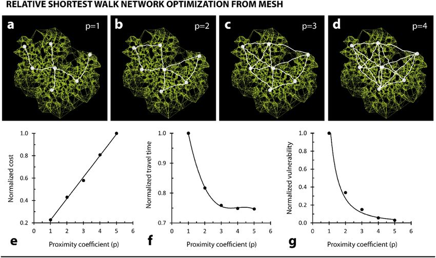
www.nature.com/scientificreports/
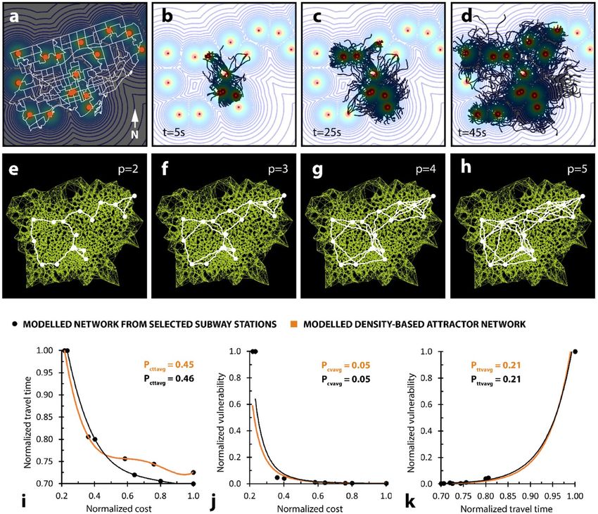
Figure 7. Built versus modelled subway network performance is varied. (a) Network to describe Toronto
underground subway system. (b–d) Modelled growth to establish mesh to describe subway system. (e–h)
Different shortest-walk calculations for the same mesh, generated from d, but with unique proximity coefficient
values. (i) Plot relating network cost to travel time for both built (orange) and modelled (black) networks.
Trendline is a fourth-order polynomial function. (j) Plot relating network cost to vulnerability for both built
(orange) and modelled (black) networks. Trendline is a power function. (k) Plot relating network travel time to
vulnerability for both built (orange) and modelled (black) networks. Trendline is an exponential function. All
performance values normalized to the largest local value. Modelled performance values displayed on the plots
represent performance for the closest modelled point to the built point (orange) along the trendline.
This is illustrated in Fig. 3d, as the attraction vector (red) grows proportionally larger, and becomes proportion-
ally more dominant compared to the stochastic “noise” vector (grey), from t = 1f to t = 3f.
Velocity magnitude was reset directly after vector summation. This enabled a constant Physarum growth
rate, but accounted for differences in force magnitude when calculating agent heading through vector summa-
tion (these differences in vector magnitude are clearly demonstrated in Fig. 3d). Food sources attracted agents
and became colonized. Figure 3 demonstrates a clustering effect around each food source, over time. Once a
given food source was depleted (we defined this event once n/10 agents reached that food source), it became
no longer attractive to the Physarum. Instead, the depleted food source became a source of offspring (providing
energy for further growth), and produced a new population of n agents, which foraged in the same manner as
described above.
Once all food sources were depleted (i.e., once all food sources were reached by n/10 agents), we terminated
the particle-growing phase of the simulation (Fig. 3e, t = 35 s). Figure 3f illustrates the agent foraging trails
throughout the complete growth process. We obtained a computationally inexpensive description of this cellular
morphology by printing the locations of these agents (as points, analogous to differentiated Physarum nuclei)
at a stepped frame rate over the duration of the simulation (one point per three frames for all simulations)
(Fig. 3g). From this cloud of nuclei points, we generated a mesh-like proximity-graph (Fig. 3h). A proximity
graph comprises a set of points (in our case, both the food sources and nuclei trail locations) and a set of edge
links that describe the proximity between all points. Here, we established the proximity graph in Fig. 3h by first
searching for two-dimensional proximity between point pairs in Fig. 3g. From this information (i.e., a distance
matrix for all pairs of points), we connected each point to its pm closest neighbours (where pm = 10 neighbours
Scientific Reports | (2022) 12:1322 | https://doi.org/10.1038/s41598-022-05439-w 8
Vol:.(1234567890)www.nature.com/scientificreports/
for all simulations). Here, pm refers to the number of neighbours to which each point was connected. What we
refer to throughout this paper as our site-responsive biased mesh (Fig. 3h) can therefore also be defined as a
10-neighbour proximity graph. The effect of pm on the density and cost of the mesh is demonstrated in Supple-
mentary Fig. S2. The density (i.e., number of linkages) in the mesh increased with pm (Supplementary Fig. S2a).
The total mesh cost also increased with pm (Supplementary Fig. S2b). This increase was determined to be linear
(Supplementary Fig. S2b, linear trendline).
Stage two: adaptive network refining. To produce a refined network (Fig. 3i), we calculated a modified
shortest-walk along the proximity graph (mesh) produced in Fig. 3h. A shortest-walk network represents the
most cost-effective (i.e., shortest) network that connects a set of points (food sources) to a certain number of its
neighbours through a given set of edges. We first searched for two-dimensional proximity between food source
pairs in order to generate a distance matrix that stored the distances between every pair of food sources. By
defining our biased mesh produced in Fig. 3h as the calculation domain (i.e., set of possible edges) for the short-
est-walk, we produced a modified shortest-walk network to connect all food sources. This network was visually
comparable to a network connecting equivalent points grown biologically (Fig. 3j,k). The network demonstrated
in Fig. 3k, for example, represents the shortest-walk network that connects each food source to a minimum of
three closest neighbours. In this case, the network in Fig. 3k can be achieved with thirteen distinct edges between
food sources. The networks produced biologically and computationally, as demonstrated in Fig. 3j,k respectively,
are compared in more detail in Fig. 5, and discussed below.
For the same set of points used to grow and computationally mesh an arbitrary network (Fig. 3a), we demon-
strated adaptive refinement control over our modelled network by establishing a proximity coefficient, p. Here, p
is used to define the number of closet neighbours to which each food source will connect, when a shortest-walk
is calculated. We demonstrated an increase in network connectivity with an increase in p (i.e., more edge con-
nections) (Fig. 4a–d). Based on network definitions given by Tero et al.20, we established three descriptions for
network efficiency, and we demonstrated the effect of p on each (Fig. 4e–g). We defined cost as the total length
of all edges within a network. We defined travel time as the average edge length required to connect two points
within a network. And we defined vulnerability as the increase in travel time for the removal of an average seg-
ment (i.e., fault) within a network. We computed this increase by systematically removing each element from
the network, calculating for each removal the average increase in network travel time. If two points became
disconnected through this calculation, we defined the distance between points as the length of the total network.
We demonstrated that network cost increased linearly (linear trendline) for an increase in proximity coefficient
(Fig. 4e). We also demonstrated that this trend was independent of the network—obtaining an identical relation-
ship for networks generated based off three randomly-generated food source sets (where the number of food
source points was set to 5, 10, and 50) (Supplementary Fig. S4). Finally, we demonstrated that both network
travel time and vulnerability decreased with an increase in proximity coefficient (Fig. 4f,g). The former trend is
described with a third-order polynomial (Fig. 4f), and the latter trend with a power function (Fig. 4g).
Effect of force constant on foraging morphology and network refinement. Supplementary
Fig. S5a illustrates the effect of force constant strength on agent trail morphology. Here, ten simulations were
run (n = 50), each with a different force constant, ranging from c = 1 to c = 1000. The relative force vector strength
increased with the force constant (Eq. 1). Therefore, the relative effect of the force vector, when summed with the
Perlin noise vector, also increased with the force constant. This resulted in a change in the noisiness of foraging:
as the force constant increased, the agents moved more deterministically and uniformly—in the direction of
the force vector (Supplementary Fig. S5a). The total trail cost (i.e., the number of agents in the foraging domain
multiplied by the runtime of the simulation) was largely independent of the force coefficient (Supplementary
Fig. S5a). The total mesh cost (described above), however, was indirectly affected by the force constant. With
a smaller force constant, trail generation was more distributed, requiring a high mesh cost to obtain appropri-
ate coverage (Supplementary Fig. S5c). The mesh cost displayed asymptotic behaviour as a function of force
coefficient (Supplementary Fig. S5c). Due to this effect, the shortest-walk (i.e., finalized network) cost was also
indirectly impacted by force coefficient. More elaborate, less cost-effective, meshes were more connected, and
provided a greater calculation domain to perform a shortest-walk. Therefore, opposite the effect on mesh cost,
shortest-walk cost increased linearly with force coefficient (Supplementary Fig. S5d).
Physarum forages both with a stochastic and sensory (i.e., deterministic) component. These are analogous,
in our model, to the Perlin noise and attractive force vector components, respectively—which we sum. The
relative magnitude of these components determines the overall distribution of the initial foraging mesh. For
example, when the force constant was low (Supplementary Fig. S5a, c = 1), the stochastic (Perlin noise) vector
was dominant in determining the agent foraging direction, resulting in a noisy forage. Oppositely, when the
force constant was high (Supplementary Fig. S5a, c = 1000), the attractive force vector was dominant in deter-
mining the agent foraging direction, resulting in a deterministic forage (here agents foraged in the direction of
the nearest food source uninterruptedly). The fraction of the foraging domain accessible (i.e., within a certain
number of pixels) to the agent trail decreased as a function of the force coefficient (Supplementary Fig. S5e–g).
This was demonstrated for three accessibility ranges: corresponding to within 20% of the total domain width
(Supplementary Fig. S5e), within 10% of the total domain width (Supplementary Fig. S5f), and within 1% of
the total domain width (Supplementary Fig. S5g). We chose to perform all simulations with a force constant of
10, as we likened the model foraging behaviour at this force constant to the foraging behaviour of the biological
organism (Supplementary Fig. S5a, c = 10).
Scientific Reports | (2022) 12:1322 | https://doi.org/10.1038/s41598-022-05439-w 9
Vol.:(0123456789)www.nature.com/scientificreports/
Effect of starting node choice on network morphology. Our multiphase model allows for high vari-
ability in the preliminary mesh with no net impact on final network morphology. The meshing stage produces an
extensive domain of trail samples for refinement, allowing for course corrections between stages. Supplementary
Fig. S6a shows seven independent meshes, developed by initializing the simulation of Physarum growth from
each of the seven unique attractor points. As can be seen, the morphology of the preliminary meshes varies
extensively. However, following the model’s network refinement stage, we see that network morphology (i.e.,
path segment similarity) is consistent across simulation iterations. This is confirmed quantitatively, as we see less
than 1% variation in cost between each of the seven networks, validating that foraging can be initialized from
any start point with no effect on final network morphology.
Model validation against biology. To compare modelled with biological growth, we conceptualized eight
unique spatial arrangements of nutrient sites (oats) atop an agar plate, and grew Physarum networks between
them. Layouts comprised a unique number of oats (ranging between 2 and 9), and, to test for variation in growth
behaviour, we repeated growth for each arrangement five times. We obtained a matrix of 40 unique networks
corresponding to the eight predesigned spatial attractor layouts (Supplementary Fig. S7a). We then digitized the
precise attractor layouts and simulated growth using our model. For consistency, we simulated Physarum growth
five times for each of the eight attractor layouts, obtaining a comparable matrix of 40 unique modelled networks.
To compare the biological and modelled Physarum networks, we first developed a methodology for simpli-
fying biological structures into refined networks. We identified the largest, most relevant veins within grown
networks by binarizing photographs taken of their form after five days, replacing each pixel (valued between 0
and 255) with either a black (255) or white (0) pixel value. We set a threshold for black–white pixel differentiation
at a pixel value of 67. This segmentation process filtered out smaller veins, and revealed the largest vein struc-
tures, which were used to define the biological network for quantitative comparison. For accurate performance
characterization and comparison, we simplified biologically-grown network geometries by fitting smooth lines
along jagged paths to eliminate foraging noise. We also neglected paths that ventured outside of the relevant
foraging boundary (i.e., towards the petri dish wall), and filtered out the more costly of two redundant paths.
This network digitization process is exemplified in Supplementary Fig. S7. Figure 5a,b compares a grown and
modelled network for one particular set of food sources with seven oats/attractor points.
To compare networks using the defined parameters of cost, travel time, and vulnerability, we defined three
general performance values, Ptt/c, Pv/c, and Pv/tt, corresponding to the normalized performance ratio between
the travel time and cost, the vulnerability and cost, and the vulnerability and travel time, respectively. Modelled
performance values are displayed in Fig. 5c–e as a best fit curve (trendline) between network results generated
with proximity coefficients between 1 and 5, while biological performance values are displayed as a point. For
the particular set of oats demonstrated in Fig. 5a,b, the grown Physarum cell performed similarly to our model,
falling within 1%, 4%, and 4% of the graphed trendline for Ptt/c, Pv/c, and Pv/tt, respectively (Fig. 5c–e): average
network travel time per cost for the Physarum was identical to the closest point along the modelled trend (1.77
versus 1.77) (Fig. 5c); average network vulnerability per cost for the Physarum was within 4% of the closest point
along the modelled trend (0.52 versus 0.50) (Fig. 5d); and average network travel time per vulnerability for the
Physarum was within 4% of the closest point along the modelled trend (0.29 versus 0.30) (Fig. 5e). It was also
observed that network morphology differences between networks modelled along the same layout of oats were
negligible, and within 1% of the cost, travel time, and vulnerability of one another.
More broadly, we compared Ptt/c, Pv/c, and Pv/tt for biological networks grown across all eight oat layouts to our
model’s corresponding performance curve (generated using 5 modelled networks, each with a different proximity
coefficient, illustrated in Supplementary Fig. S7b). P tt/c, Pv/c, and Pv/tt for each of the five grown networks were
compared to the closet point along the modelled curve. The differences in Ptt/c, Pv/c, and Pv/tt between grown and
modelled networks are shown in Fig. 5f–h, respectively. Despite observable trends in morphology differences
between grown and modelled networks (e.g., n = 3 in Supplementary Fig. S7), performance discrepancy values
never exceeded 4%. This result is partly explained by performance metric dependence, where more costly net-
works tended to have lower travel times and vulnerabilities, while cheaper networks tended to have higher travel
times and vulnerabilities. In 55%, (22/40) of the growth iterations, grown networks were directly identical to a
modelled counterpart (such a case results in a 0% difference in P tt/c, Pv/c, and P
v/tt, and is particularly common
for n = 2, 4–6). The remaining grown networks performed, on average, within 0.4%, 0.8%, and 0.7% of the P tt/c,
Pv/c, and Pv/tt curves of their modelled equivalents, respectively, confirming broad agreement between systems.
Model comparison to urban infrastructure. We used our model to generate networks that describe two
existing systems of urban infrastructure at two scales: an amusement park (Canada’s Wonderland in Toronto,
Ontario), and a subway system (Toronto Transit Corporation Subway system in Toronto, Canada). From an
aerial photograph of Canada’s Wonderland, we digitized selected attraction points (food sources) and edge con-
nections (network) (Fig. 6a). We used these digitized attractor points to generate a nutrient domain to model
Physarum growth (Fig. 6b–d). We produced several network iterations, for unique proximity coefficient values
(Fig. 6e–h). We compared modelled with built network performance (Fig. 6i–k). Our modelled network per-
formed more favourably over the existing network, displaying 27% lower P ctt (cost × travel time) (0.37 ver-
sus 0.47) (Fig. 6i), 61% lower Pcv (cost × vulnerability) (0.29 versus 0.47) (Fig. 6j), and 2% lower Pttv (travel
time × vulnerability) (0.99 versus 0.98) (Fig. 6k). As before, modelled P ctt, Pcv, and P ttv values were calculated
from the closest point to the urban network along the modelled trendline.
We obtained spatial data of the four subway lines and 74 stations that make up the underground subway
network in Toronto, Canada, and we selected seventeen core stations to represent network attractors (Fig. 7a).
We modelled a network to represent Physarum growth across the seventeen core subway stations (Fig. 7b–h),
Scientific Reports | (2022) 12:1322 | https://doi.org/10.1038/s41598-022-05439-w 10
Vol:.(1234567890)www.nature.com/scientificreports/
Figure 8. Comparison between modelled networks generated with population-density- and subway-station-
defined attractor points. (a) Dot density population distribution of city of Toronto, where each dot represents
150,000 residents (b–d) Modelled growth to establish mesh to describe hypothetical subway system, based off
attractors generated in a. (e–h) Different shortest-walk calculations for the same mesh, generated from d, but
with unique proximity coefficient values. (i) Plot relating network cost to travel time for both density-based
network model (orange) and station-based network model (black). Trendlines are both fourth-order polynomial
functions. (j) Plot relating network cost to vulnerability for both density-based network model (orange) and
station-based network model (black). Trendlines are both power functions. (k) Plot relating network travel
time to vulnerability for both density-based network model (orange) and station-based network model (black).
Trendlines are both exponential functions. All performance values normalized to the largest local value.
Modelled average performance values displayed on the plots represent average performance values cross all
network iterations.
and compared modelled with built network performance (Fig. 7i–k). Our modelled network performed differ-
ently compared to the existing subway system, displaying 14% higher P ctt (cost × travel time) (0.26 versus 0.22)
(Fig. 7i), identical P
cv (cost × vulnerability) (0.13 versus 0.13) (Fig. 7j), and 19% lower P ttv (travel time × vulner-
ability) (0.41 versus 0.49) (Fig. 7k). As before, modelled P ctt, Pcv, and P
ttv values were calculated from the closest
point to the urban network along the modelled trendline.
Population density‑defined attractor network. We demonstrated that networks can be generated not
only from predefined points of interest, but from various forms of spatial data that are interpretable as a set of
attractor points. We used population data for neighbourhoods in Toronto, Canada to generate seventeen attrac-
tor points that represented the population distribution of the city (i.e., each point represents 150,000 residents)
(Fig. 8a). We simulated Physarum growth across this set of points (Fig. 8b–d), and generated alternative subway
networks for unique proximity values (Fig. 8e–h). We compared network performance between density-gener-
ated attractors and station-generated attractors (Fig. 8i–k). Modelled performance was nearly identical across
the two systems. The population density-defined network displayed 2% lower P cttavg (average cost × travel time)
(0.45 versus 0.46) (Fig. 8i), 5% lower Pcvavg (average cost × vulnerability) (495e−4 versus 524e−4) (Fig. 8j), and
1% higher Pttvavg (average travel time × vulnerability) (211e−3 versus 209e−3) (Fig. 8k).
Scientific Reports | (2022) 12:1322 | https://doi.org/10.1038/s41598-022-05439-w 11
Vol.:(0123456789)www.nature.com/scientificreports/
Discussion
We implemented a discrete, two-phase Physarum model that leveraged independent mechanisms to generate both
a mesh and final network responsive to the attractor field in which they were established. We demonstrated that
this biologically-inspired model, despite omitting the biological constructive feedback mechanism that enables
growth, could accurately describe plasmodial Physarum growth to within 4% and, moreover, that it could be lev-
eraged more directly as a simple tool to design networks comparable to existing systems of urban infrastructure.
We conclude that network performance, defined using cost, travel time, and vulnerability, between our grown
and modelled Physarum systems was highly similar (within 4% across various attractor layouts and growth
iterations). We also conclude that network performance varied between our modelled Physarum system and
existing urban infrastructure systems. The discrepancies in this performance can prove to be highly informa-
tive, serving to illuminate strengths, susceptibilities, and overarching design differences between biological and
anthropic networking systems. For example, our bio-inspired model performed superiorly in all measurable
categories compared to Canada’s Wonderland. For an equivalent cost, we generated a network that was over 80%
less vulnerable (Fig. 6j) and almost 10% less time-consuming (Fig. 6i) than the existing system. This difference
may be because amusements parks have different design goals to conventional transportation systems—where
excess costs and travel times may be considered favourable (e.g., a greater path network to land area ratio may
increase consumer opportunities). Our bio-inspired model performed less favourably in some measurable cat-
egories compared to a more conventional transportation system—Toronto’s underground subway network. For
an equivalent cost, we generated a network that was identically vulnerable to fault (Fig. 7j), but almost 10% more
time-consuming (Fig. 7i) than the existing subway system. For an equivalent travel time, however, we generated a
network that was about 40% less vulnerable to fault than the existing subway system (Fig. 7k). Biological organ-
isms are characteristically resilient, able to regenerate and adapt to faults. This model may serve as a basis for
more resilient network construction—which is becoming increasingly relevant with the unpredictable impacts
of climate change.
When comparing grown and modelled networks, graphs in Fig. 5g,h demonstrate two small peaks in per-
formance difference occurring at n = 3 and between n = [6, 9]. The discrepancies between layouts n = [6, 9] can
most likely be explained by the increasing complexity of the grown networks and greater range in decision
making variability of the organism. The discrepancies between networks grown within the attractor layout of
n = 3 (triangle shape), on the other hand, may point to an important limitation in the model. In 3 of 5 growth
iterations, the organism formed a Steiner minimum tree between oats, a result that differs from the complete or
near-complete triangle morphologies produced by our model. This discrepancy emphasizes the limited number
of discrete proximity coefficient steps the model can choose between, unable to find optimized network solutions
using paths that do not directly link two attractor points. Such a limitation is less important as networks increase
in complexity, but may bound efficient growth to a minimum oat layout of n = 4.
Compared to other models, our work enables multi-objective (e.g., cost, travel time, vulnerability) network
design, independent of preliminary growth. Networking systems across various scales, built for various environ-
mental and functional regimes, must also adhere to complex and competing constraints, and may also benefit
from late-stage, multi-objective design control. Relative to existing models, our stepwise algorithm omits critical
feedback loops of streaming behaviour, limiting its effectiveness capturing the characteristics and morphological
dynamics of Physarum growth. Instead, our model emphasizes broad applicability: compared to nearly all current
models, which do not allow for stepwise interruption and tuning, our work offers an opportunity for designer
feedback and input amidst the growth process, enabling new avenues for applied network generation. Addition-
ally, our model allows for flexibility in starting condition. Diverging from the behaviour of live Physarum, and
the many models that draw from it, our algorithm demonstrates consistent network results independent of the
point from which growth was initialized. We therefore imagine that the presented model will prove especially
useful for applications where design objectives are strict (e.g., in situations where start node cannot be controlled,
or where more ‘biologically-accurate’ Physarum models cannot produce network morphologies within a tight
application domain).
Our model specifically enables network growth from attractor-based information. Networks can be estab-
lished through simple data translation (e.g., population distribution as attractors, information density distribu-
tion as attractors, physical boundaries as anti-attractors) from the urban to the microelectronic network scale.
Importantly, we note that our model currently functions in ‘idealized’ environments with attractors, and does not
include repellants (anti-attractors). It is not clear how Physarum negotiates environments where both attractors
and anti-attractors are present. For instance, many of the complex behaviours exhibited by Physarum cannot be
explained by simple stimulus–response models58. In one set of physical experiments, when Physarum was intro-
duced to bi-modal stimuli—consisting of a standard mixture of both attractor and anti-attractor materials—the
plasmodium varied its decision-making and network morphologies. For the same attractor concentration, the
organism was inconsistently attracted to the stimuli, at times even completely avoiding the stimuli58. Developing
more advanced models that can function in environments with both attractors and anti-attractors would be a
be a beneficial future endeavour.
Additionally, from our existing proximity graph model, it will be easy to develop networks that adapt their
path segment capacities depending on usage. Path segments can take on diameters proportional to their use
frequency, where frequency can be determined while calculating shortest network travel times between point
pairs. This added dimension of network morphology would enable more broad applicability—to solve flux-based
and path-planning problems simultaneously.
Perhaps most fundamentally, this work provides a simple baseline for developing and quantitatively assessing
network performance at the urban scale. Infrastructural networks are too often constructed without standard
and quantitative design principles, and the model described here can help benchmark both existing and future
Scientific Reports | (2022) 12:1322 | https://doi.org/10.1038/s41598-022-05439-w 12
Vol:.(1234567890)www.nature.com/scientificreports/
network developments towards achieving more efficient and resilient cities. Additionally, we note that the step-
wise principles of growth introduced here may find relevant applications in other network problems across
multiple length-scales, representing exciting trajectories for future inquiry.
Conclusions
Physarum can operate as a biological computer, and is particularly useful for solving anthropically-shared prob-
lems of transport network design. We characterized Physarum growth as a two-phase process (biased meshing
and network refining), and described such behaviour with a two-phase digital model. Our model produced
networks that performed nearly identically to the biological organism, but differently to existing urban infra-
structure. This model enables tunable, multi-objective network design, independent of the environmental regime.
As such, it can serve as an urban design tool that offers biologically-informed rules for network construction.
Materials and methods
Sample preparation and imaging. Physarum polycephalum (Carolina Biological Supply) was grown on
1.5% (weight/volume) nutrient-free agar (BioShop), prepared in a 9-cm-diameter polystyrene petri dish (VWR).
Oat flakes (Carolina Biological Supply) were placed across the substrate in a predesigned pattern, and the active
plasmodium (approx. 2-mm-diameter sphere) was placed atop a prespecified oat. Cardstock cutouts were used
to ensure consistent oat placement for repeated experiments. Additional oat flakes were placed around the plas-
modium to accelerate growth. Samples were stored in low-light, room-temperature conditions, except during
imaging. Samples were imaged daily with a Nikon D3200 DSLR camera, and illuminated from below (Fig. 2a).
Additional imaging was obtained after 2, 4, 7, and 12 days, using a BW500 digital microscope (Fig. 1m–o, Sup-
plementary Fig. S1e,f) and AmScope MU1000 microscope digital camera (Fig. 1c–j).
Image digitization. We converted digital photographs, taken of the organism and substrate after 5 and
7 days, into points (attractor points) and vectors (network edges). Images were analyzed using ImageJ software
(National Institutes of Health. Bethesda, MD, United States), and vectorized in Adobe Illustrator (Adobe. San
Jose, CA, United States). For identifying relevant paths from network photographs, images were binarized using
a specified black–white pixel value threshold in ImageJ. Point data was used to establish input attractor point
information. Vectorization was also used to interpret urban infrastructural networks (Fig. 5a).
Model development. We developed an agent-based model in Processing (M.I.T. Cambridge, MA, United
States). Agent locations, stored as points, were exported into the modelling environment Rhinoceros (Robert
McNeel & Associates. Seattle, WA, United States). All network refinement (shortest-walk calculations) and net-
work analysis was done in Grasshopper, a visual coding plugin for Rhinoceros (Robert McNeel & Associates.
Seattle, WA, United States). We used Grasshopper to translate modelled network segments into simplified line-
work, for more efficient network assessment.
Data acquisition. Spatial transportation and population data was obtained from the Toronto Police Ser-
vices (City of Toronto Open Data Portal). Attractor points that represented population density were calculated
as dot density data points in ArcMap (Esri. Redlands, CA, United States).
Data availability
No datasets were generated or analyzed during the current study. All code can be made available by the cor-
responding authors upon request.
Received: 5 May 2021; Accepted: 6 January 2022
References
1. Takamatsu, A., Takaba, E. & Takizawa, G. Environment-dependent morphology in plasmodium of true slime mold Physarum
polycephalum and a network growth model. J. Theor. Biol. 256, 29–44. https://doi.org/10.1016/j.jtbi.2008.09.010 (2009).
2. Nakagaki, T., Yamada, H. & Hara, M. Smart network solutions in an amoeboid organism. Biophys. Chem. 107, 1–5. https://doi.
org/10.1016/s0301-4622(03)00189-3 (2004).
3. Zhu, L., Aono, M., Kim, S. J. & Hara, M. Amoeba-based computing for traveling salesman problem: Long-term correlations between
spatially separated individual cells of Physarum polycephalum. Biosystems 112, 1–10. https://doi.org/10.1016/j.biosystems.2013.
01.008 (2013).
4. Adamatzky, A. Physarum Machines Vol. 74 (World Scientific, 2010).
5. Alim, K., Andrew, N., Pringle, A. & Brenner, M. P. Mechanism of signal propagation in Physarum polycephalum. Proc. Natl. Acad.
Sci. 114, 5136. https://doi.org/10.1073/pnas.1618114114 (2017).
6. Ueda, T., Hirose, T. & Kobatake, Y. Membrane biophysics of chemoreception and taxis in the plasmodium of Physarum polycepha-
lum. Biophys. Chem. 11, 461–473. https://doi.org/10.1016/0301-4622(80)87023-2 (1980).
7. Reid, C. R., Latty, T., Dussutour, A. & Beekman, M. Slime mold uses an externalized spatial “memory” to navigate in complex
environments. Proc. Natl. Acad. Sci. 109, 17490. https://doi.org/10.1073/pnas.1215037109 (2012).
8. Durham, A. C. & Ridgway, E. B. Control of chemotaxis in Physarum polycephalum. J. Cell Biol. 69, 218–223. https://doi.org/10.
1083/jcb.69.1.218 (1976).
9. Alim, K., Amselem, G., Peaudecerf, F., Brenner, M. P. & Pringle, A. Random network peristalsis in Physarum polycephalum organ-
izes fluid flows across an individual. Proc. Natl. Acad. Sci. U. S. A. 110, 13306–13311. https://doi.org/10.1073/pnas.1305049110
(2013).
10. Wohlfarth-Bottermann, K. E. Oscillating contractions in protoplasmic strands of Physarum: Simultaneous tensiometry of longi-
tudinal and radial rhythms, periodicity analysis and temperature dependence. J. Exp. Biol. 67, 49 (1977).
Scientific Reports | (2022) 12:1322 | https://doi.org/10.1038/s41598-022-05439-w 13
Vol.:(0123456789)You can also read