The Mainz profile algorithm (MAPA) - Atmos. Meas. Tech
←
→
Page content transcription
If your browser does not render page correctly, please read the page content below
Atmos. Meas. Tech., 12, 1785–1806, 2019
https://doi.org/10.5194/amt-12-1785-2019
© Author(s) 2019. This work is distributed under
the Creative Commons Attribution 4.0 License.

The Mainz profile algorithm (MAPA)
Steffen Beirle, Steffen Dörner, Sebastian Donner, Julia Remmers, Yang Wang, and Thomas Wagner
Max-Planck-Institut für Chemie (MPI-C), Satellitenfernerkundung, Mainz, Germany

Correspondence: Steffen Beirle (steffen.beirle@mpic.de)

Received: 23 October 2018 – Discussion started: 22 November 2018
Revised: 28 January 2019 – Accepted: 11 February 2019 – Published: 19 March 2019

Abstract. The Mainz profile algorithm (MAPA) derives ver-        Wagner et al., 2004; Wittrock et al., 2004; Frieß et al., 2006;
tical profiles of aerosol extinction and trace gas concentra-    Clémer et al., 2010), which is key for the validation of trace
tions from MAX-DOAS measurements of slant column den-            gas columns derived from satellite measurements.
sities under multiple elevation angles. This paper presents         MAX-DOAS is based on the elevation angle dependency
(a) a detailed description of the MAPA (v0.98), (b) results      of spectral absorption, i.e., the differential slant column den-
for the CINDI-2 campaign, and (c) sensitivity studies on the     sity (dSCD) determined by DOAS (Platt and Stutz, 2008).
impact of a priori assumptions such as flag thresholds.          The profile retrieval is performed in two steps: first, aerosol
   Like previous profile retrieval schemes developed at          extinction profiles are derived based on dSCDs of the oxy-
MPIC, MAPA is based on a profile parameterization combin-        gen dimer O4 . In a second step, the concentration profiles
ing box profiles, which also might be lifted, and exponential    of various trace gases detectable in the UV–vis range (such
profiles. But in contrast to previous inversion schemes based    as nitrogen dioxide, NO2 , and formaldehyde, HCHO) can be
on least-square fits, MAPA follows a Monte Carlo approach        determined.
for deriving those profile parameters yielding best match to        For given aerosol and trace gas profiles, dSCDs of O4 and
the MAX-DOAS observations. This is much faster and di-           atmospheric trace gases can be modeled by radiative trans-
rectly provides physically meaningful distributions of profile   fer models (RTMs) for a sequence of elevation angles. The
parameters. In addition, MAPA includes an elaborated flag-       “profile inversion” consists of inverting this forward model,
ging scheme for the identification of questionable or dubious    i.e., finding the extinction and concentration profile where
results.                                                         forward modeled and measured dSCD elevation sequences
   The AODs derived with MAPA for the CINDI-2 campaign           agree.
show good agreement with AERONET if a scaling factor of             Profile inversion can be carried out based on a regular-
0.8 is applied for O4 , and the respective NO2 and HCHO sur-     ized matrix inversion method denoted as optimal estima-
face mixing ratios match those derived from coincident long-     tion (Rodgers, 2000). It provides an elaborated mathemat-
path DOAS measurements. MAPA results are robust with re-         ical framework yielding the best extinction and concentra-
spect to modifications of the a priori MAPA settings within      tion profile estimate and the corresponding averaging kernels
plausible limits.                                                for a given measurement and a priori error (e.g., Frieß et al.,
                                                                 2006; Clémer et al., 2010). However, results depend on the a
                                                                 priori settings, in particular the a priori profile and its uncer-
                                                                 tainty, which are generally not known.
1   Introduction                                                    An alternative approach involves parameterized profiles
                                                                 (Irie et al., 2008; Li et al., 2010; Wagner et al., 2011; Vlem-
Multi-axis differential optical absorption spectroscopy          mix et al., 2011, 2015). The basic idea is to represent vertical
(MAX-DOAS), i.e., spectral measurements of scattered sun-        profiles with a few parameters, typically representing total
light under different viewing elevation angles, has become       column, height, and shape. The profile inversion then corre-
a useful tool for the determination of vertical profiles of      sponds to finding the best matching parameters. Due to the
aerosols and various trace gases within the lower troposphere    limited number of parameters, a regularization as used in op-
(e.g., Hönninger and Platt, 2002; Hönninger et al., 2004;

Published by Copernicus Publications on behalf of the European Geosciences Union.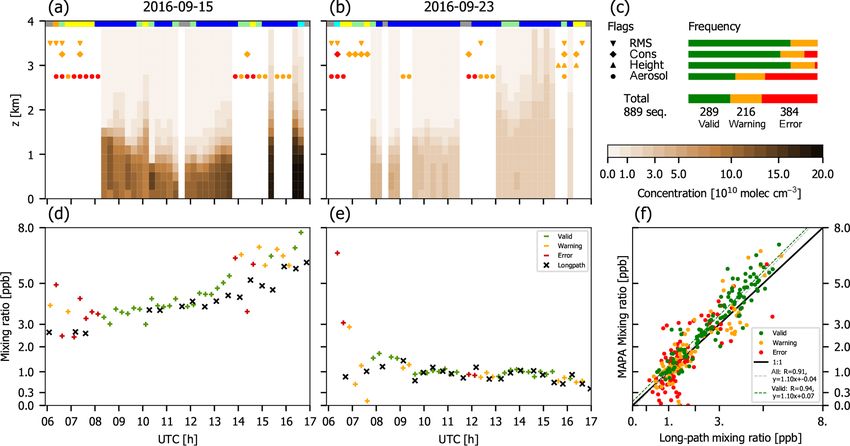
1786                                                                                                     S. Beirle et al.: MAPA

timal estimation is not required, and the method makes no a       The measurement principle is shortly described in Sect. 2.2.
priori assumptions on the actual profile (except that its shape   In Sect. 2.3, the required input to the MAPA is specified. Sec-
can be represented by the chosen parameterization).               tion 2.4 describes the profile parameterization. In Sect. 2.5,
   So far, parameter-based inversion has used nonlinear least-    the forward model, linking profile parameters to elevation
squares algorithms like the Levenberg–Marquardt algorithm         sequences of dSCDs, is provided. The profile inversion al-
(LMA). This is an established method. However, it has some        gorithm is described in Sect. 2.6. Section 2.7 deals with the
drawbacks: first, the LMA is based on local linearization,        O4 scaling factor (SF). Finally, the flagging procedure, in or-
while the forward model is typically highly nonlinear in the      der to identify questionable results and outliers, is explained
parameters. As a consequence, the confidence intervals (CIs)      in Sect. 2.8.
resulting from the LMA are symmetric by definition and of-
ten result in unphysical values of the fitted parameter ± CI,     2.1   Heritage and advancements
like a negative layer height. Second, the profile parameters
are often strongly correlated, i.e., different parameter combi-   MAPA is founded on the parameterized profile inversion ap-
nations can result in similar profile shapes. This implies the    proach described in Li et al. (2010) or Wagner et al. (2011). It
existence of local minima in the minimization task, making        uses profile parameter definitions similar to those of Wagner
the LMA challenging and slowing down the inversion.               et al. (2011) and forward models linking those parameters to
   Here we present an alternative parameter-based inversion       dSCD sequences.
method using a Monte Carlo (MC) approach: the (finite)               The main advancements of MAPA compared to Wagner et
space of parameter combinations is covered by random num-         al. (2011) are that
bers, and those best matching the measurement are kept. This        – MAPA is completely rewritten from scratch in Python.
approach directly yields distributions rather than single es-
timates for each parameter, thereby accounting for the cor-         – all settings are easily adjustable by separate configura-
relation of parameters. In addition, the distributions do not         tion files.
contain unphysical parameters (as occur for the LMA best
                                                                    – MAPA provides the option of a variable scaling factor
estimates ± CI).
                                                                      for O4 (see Sect. 2.7).
   The MC approach used in MAPA v0.98 is much faster than
the previous LMA implementation. In addition, the informa-          – MAPA uses a Monte Carlo approach for the profile in-
tion on a distribution of the best matching parameters allows         version (see Sect. 2.6.2), while Wagner et al. (2011)
for a straightforward determination of the vertical concentra-        used the LMA. The MC approach is faster and provides
tion profiles and their uncertainties. The algorithm can also         physically meaningful uncertainty information.
be easily adopted to additional or different profile parameter-
izations.                                                           – MAPA provides an elaborated flagging scheme for the
   MAPA is included as representative of parameter-based              identification of questionable results (Sect. 2.8).
algorithms in the processing chain of Fiducial Reference             In the sections below we provide a full description of
Measurements for Ground-Based DOAS Air-Quality Obser-             the MAPA profile inversion algorithm, also including parts
vations (FRM4DOAS), a 2-year ESA project which started            which have been described before (like the profile parame-
in July 2016 (http://frm4doas.aeronomie.be/, last access:         terization) for sake of clarity and completeness.
18 February 2019).
   In this paper, the MAPA v0.98 is described in Sect. 2.         2.2   MAX-DOAS
Exemplary results for the CINDI-2 campaign are shown in
Sect. 3. The dependency of MAPA results on a priori set-          With DOAS, the slant column density (SCD), i.e., the inte-
tings as well as clouds is investigated in Sect. 4. The limita-   grated column along the effective light path, can be deter-
tions of profile inversions from MAX-DOAS measurements            mined from spectral measurements of scattered sunlight for
in general and MAPA in particular are discussed in Sect. 5,       molecules with absorption structures in the UV–vis spectral
followed by conclusions.                                          range (Platt and Stutz, 2008). The SCD can be converted into
   Appendix A lists the abbreviations used within this study      a vertical column density (VCD), i.e., vertically integrated
(Table A1) and the mathematical symbols used for variables        column, by division with the so-called air mass factor.
and parameters (Table A2).                                           MAX-DOAS measurements are performed from ground-
                                                                  based spectrometers with different elevation angles (EAs) α,
                                                                  including zenith sky measurements, in order to derive profile
2   Method                                                        information from the EA dependency of slant column densi-
                                                                  ties.
In this section, we describe the MAPA profile inversion al-          By using the zenith measurements before and/or after a
gorithm. First, the similarities and differences to existing      sequence of different EAs as reference spectrum within the
parameter-based inversion schemes are outlined in Sect. 2.1.      DOAS analysis, the so-called dSCD S, representing the SCD

Atmos. Meas. Tech., 12, 1785–1806, 2019                                             www.atmos-meas-tech.net/12/1785/2019/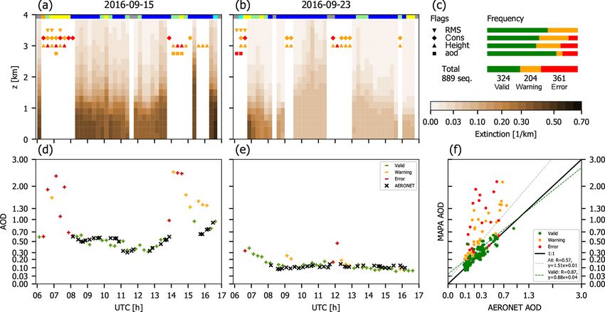
S. Beirle et al.: MAPA 1787
excess compared to zenith viewing geometry, is derived. 2.4 Profile parameterization
Analogously, the differential air mass factor (dAMF) A re-
lates the dSCD S to the VCD V : Within MAPA, vertical profiles p(z) of aerosol extinction
and trace gas concentration are parameterized by three pa-
V = S/A. (1) rameters, similar to Wagner et al. (2011):
1. the integrated column c (i.e., AOD for aerosols, VCD
Note that the DOAS spectral analysis is not part of MAPA for trace gases),
but has to be carried out beforehand.
2. the layer height h, and
2.3 Input
3. the shape parameter s ∈]0, 2[.
Here we list the basic quantities needed as input for MAPA. A shape parameter of s = 1 represents a simple box pro-
A detailed description of the MAPA input file format is pro- file:
vided at ftp://ftp.mpic.de/MAPA/. (
c/ h for z ≤ h
p(z)c,h,s=1 = (2)
2.3.1 Viewing and solar angles 0 for z > h.
The geometry has to be specified in the MAPA input data, For a shape parameter of 0 < s < 1, the fraction s of the
defined by the EA α, the solar zenith angle (SZA) ϑ, and total column c is placed within a box. The remaining fraction
the relative azimuth angle (RAA) ϕ between viewing direc- (1 − s) exponentially declines with altitude:
tion and direction of the sun. Absolute (solar and viewing)
azimuth angles are not needed.
(
s × c/ h for z ≤ h
p(z)c,h,s h
(3)
A sequence of i = 1. . .M EAs with corresponding dSCDs
Si = S(αi ) is required for one profile to be retrieved. Below, A shape parameter of 2 > s > 1 represents an elevated
a dSCD sequence is noted as vector S, where the ith com- layer from h1 to h of thickness h2 :
ponent corresponds to αi . Note that the dependency on α is
implicit in all vectors below and not written explicitly any 0
for z < h1
more. p(z)c,h,s>1 = c/h2 for h1 < z ≤ h , (4)
In addition, the corresponding sequence of the DOAS fit
0 for z > h
error S err is required. We define the typical dSCD error Serr
as the sequence median DOAS fit errors. with
As aerosol profiles have to be retrieved first as a prereq-
h1 = (s − 1)h
uisite for trace gas inversions, each MAPA input file must
h2 = (2 − s)h. (5)
contain at least one dataset of O4 dSCDs. In addition, trace
h1 + h2 = h
gas dSCD sequences can be included as needed.
Equations (3) and (4) converge to a box profile for s → 1;
2.3.3 O4 VCD thus Eqs. (2) to (4) describe a set of parameterized profiles
which are continuous in s. Figure 1 exemplarily displays ex-
For the MAPA aerosol retrieval, an a priori O4 VCD VO4 is tinction profiles for c = 1 and different heights h and shape
required for each sequence in order to relate the measured parameters s.
O4 dSCDs to O4 dAMFs (see Eq. 1 and Sect. 2.5). VO4 can Alternative parameterizations (like a linear increase from
be provided explicitly in the input data. If missing, it is cal- the ground to h (compare Wagner et al., 2011) or even com-
culated from temperature and pressure profiles. If full profile pletely different profile shapes) might be used instead or
measurements are provided in the input, they are used. If only in addition in future MAPA versions. This would require
ground measurements at the station are available, they are the calculation of corresponding look-up tables (LUTs) for
used to construct extrapolated profiles based on a constant dAMFs (see below).
lapse rate of up to 12 km and a constant temperature above
(see Wagner et al., 2018, Sect. 4.1.1, for details). If no tem- 2.5 Forward model
perature and pressure information is provided in the MAPA
input, ERA-Interim data (Dee et al., 2011) from the European In this section the forward model (fm) is specified, which
Centre for Medium-Range Weather Forecasts (ECMWF) is connects the profile parameters c, h, and s, with dSCDs for
used for the calculation of VO4 . the given solar and viewing geometry.
www.atmos-meas-tech.net/12/1785/2019/ Atmos. Meas. Tech., 12, 1785–1806, 2019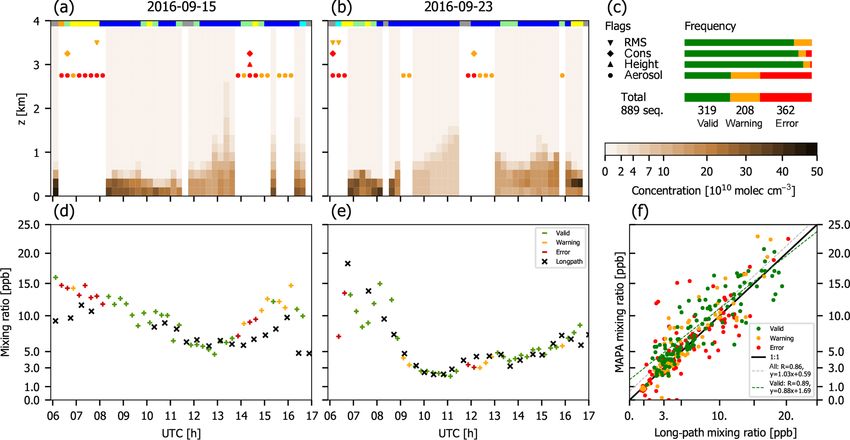
1788                                                                                                                     S. Beirle et al.: MAPA

Figure 1. Illustration of the profile parameterization. Aerosol extinction profiles are shown for caer ≡ τ = 1, different heights h (color coded),
and shape parameters s = 0.7 (a), 1.0 (b), and 1.3 (c).

   Essentially, the forward model is given by Eq. (1): S =                 2.5.2      Forward model for trace gases
V × A, where the dAMF depends on profile parameters and
solar and viewing geometry. Within MAPA, dAMFs have                        For trace gases, the dAMFs also depend on the aerosol profile
been calculated offline with the radiative transfer model                  parameters as determined from the analysis of O4 dSCDs1
McArtim (Deutschmann et al., 2011) for fixed nodes for each                but not on the trace gas VCD ctg , as long as optical depths
parameter and stored as a LUT. Within MAPA profile inver-                  are low (which is a prerequisite for DOAS analysis):
sion, these multidimensional LUTs are interpolated linearly
for the given parameter values. For details on the dAMF LUT                Atg = f (htg , stg )|ϑ,ϕ,caer ,haer ,saer .                        (8)
properties see Appendix B.
   Note that the profile parameterization (Sect. 2.4) is the                  The corresponding dSCD is
same for aerosols and trace gases. The forward models for                    tg
aerosols and trace gases, however, are similar (and the pro-               S fm = V tg × Atg = ctg × Atg .                                    (9)
file retrieval is based on the same code as far as possible) but
not identical. This is due to the fact that the column param-              The trace gas VCD V tg is identical to the column parameter
eters caer and ctg have different meanings in the context of               ctg .
S and V : for aerosols, c equals the AOD τ , which is com-
                                                                           2.6     Profile inversion
pletely independent of the O4 VCD. For trace gases, c equals
the VCD Vtg .                                                              The forward model as defined above translates the aerosol
   Below, the forward models will be described for both O4                 and trace gas profile parameters c, h, and s into dSCD se-
(which is the basis for retrieving aerosol profiles) and trace             quences S fm . Within profile inversion, the task is now to find
gases.                                                                     those model parameters yielding the “best match” (bm) be-
                                                                           tween S fm and the measured dSCD sequence S ms . Typically,
2.5.1    Forward model for aerosols                                        best match is defined in terms of least squares of the residue;
                                                                           i.e., the root mean square (RMS)
For aerosols, the O4 dAMF is a direct function of the profile                     s
parameters caer (≡ τ ), haer , saer and viewing geometry ϑ, ϕ:                        (S fm − S ms )2
                                                                           R=                                                                (10)
                                                                                            M
AO4 = f (caer , haer , saer )|ϑ,ϕ .                               (6)
                                                                           is minimized, with M being the number of EAs (i.e., the
                                                                           length of S).
   The corresponding dSCD is                                                  In previous parameter-based inversion schemes, the best
                                                                           matching parameters have been determined by nonlinear
SO 4    O4         O4
 fm = Va priori × A .                                             (7)      least-squares algorithms like the Levenberg–Marquardt algo-
                                                                           rithm (Li et al., 2010; Wagner et al., 2011; Vlemmix et al.,
                                                                           2015). This approach, however, has some drawbacks, in par-
  The respective VCD of O4 (or vertical profiles of pres-
                                                                           ticular
sure and temperature, which allow for the calculation of VO4 )
has to be provided in the MAPA input or is calculated from                    1 Note that it is not possible to directly use an a priori vertical
ECMWF profiles.                                                            aerosol extinction profile within MAPA trace gas inversion.

Atmos. Meas. Tech., 12, 1785–1806, 2019                                                           www.atmos-meas-tech.net/12/1785/2019/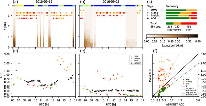
S. Beirle et al.: MAPA                                                                                                               1789

  – as the parameters are highly correlated and local minima         2.6.2   Other profile parameters: Monte Carlo
    can exist, high computational effort, i.e., multiple mini-
    mization calls with different initial values, is needed in       Within MAPA, profile parameters are determined by just
    order to soundly determine the absolute minimum.                 covering the parameter space by random numbers2 and keep-
                                                                     ing the matches. In detail, the following steps are performed:

  – as the least-squares algorithms are based on local lin-            1. limits are defined for each parameter3 ,
    earization, the resulting parameter uncertainties are per          2. ntot sets of random parameters are drawn4,5 ,
    construction symmetric; the resulting parameter range
    spanned by the fitted parameter ± CI is often unphysi-             3. the RMS R is calculated for each random parameter set,
    cal (e.g. h < 0 or s > 2) and thus meaningless.
                                                                       4. the lowest RMS is identified as best match (bm) Rbm ,
                                                                          and
Within MAPA (from v0.6 onwards), a different approach
based on the Monte Carlo (MC) method is chosen. The idea               5. an ensemble of up to nsel parameter sets with R/Rbm <
is to (a) generate multiple random sets of profile parameters,            F is kept.
(b) calculate the respective dSCD and RMS, and (c) keep
those yielding the best agreement. This approach results in             Table 1 lists the default values for parameter limits, num-
a best matching set of parameters, plus an ensemble of pa-           ber of random samples, and thresholds for MAPA v0.98. The
rameter sets with similar low R, which reflects the uncer-           impact of variations of these settings is discussed in Sect. 4.1.
tainty range of the estimated profile parameters, which per             The steps listed above are iterated three times, for which
construction only contains physically valid values.                  the resulting ensemble is used to narrow down the parameter
    Section 2.6.2 describes the details of the MC inversion          limits for the next iteration. That is, if the lowest RMS values
approach, which is used for the determination of h, s, and           are always found for low s, the limits for s will be narrowed
caer . Before that, in Sect. 2.6.1 the determination of ctg is de-   for the next iteration. As the total number of random samples
scribed, which is implemented differently by a simple linear         stays the same, this procedure results in increasingly finer
fit.                                                                 spacing of random numbers.
                                                                        The procedure results in a best matching parameter set,
2.6.1   VCD: linear fit                                              plus an ensemble of acceptable parameter sets. For each pa-
                                                                     rameter set, the corresponding VCD Vbm is also determined
                                                                     by Eq. (11).
The dSCD forward model is highly nonlinear in h and s and
also in AOD caer . These parameters are derived by a MC ap-          2.6.3   Best match and ensemble statistics
proach as described in detail in the next section.
   The trace gas VCD ctg , however, is just a scaling factor of      MAPA yields the best matching parameter combination. The
A (Eq. 9). Thus, for a given set of profile parameters, and a        corresponding vertical profile is given by Eqs. (2)–(4). In
given sequence of measured dSCDs, the best matching trace            addition, MAPA yields an ensemble of parameter sets with
gas VCD ctg = Vbm can just be determined by a linear fit             R < F × Rbm , i.e., similar (slightly worse) agreement be-
(forced through origin) of V :                                       tween measurement and forward model. From this ensem-
                                                                     ble, the following statistics are derived for both the profile
        S ms · A                                                     parameters and the corresponding vertical profiles:
Vbm =            .                                           (11)
         A·A                                                           – weighted mean (wm) and standard deviation, with 1/R 2
                                                                         as weights;
(Note that S and A are vectors, and the multiplications are
scalar products.)                                                      – 25 and 75 percentiles; and
   In other words, the best matching V equals the mean of Vi            2 MAPA also provides the option to fix each of the parameters to
for individual elevation angles, weighted by the respective
                                                                     a predefined value.
dAMF (i.e., sensitivity). This is different from Wagner et al.           3 This approach (as well as the implementation of the dAMF as
(2004), in which V was calculated as the simple mean of Vi
                                                                     a LUT) is only possible since the (physical or plausible) parameter
for the individual elevation angles without weighting.               ranges are limited.
   The same formalism is used to define a VCD uncertainty                4 By default the random number generator is initialized with a
Verr as the weighted mean of dSCD errors (from DOAS anal-            seed β in order to generate reproducible results.
ysis) for individual EAs. Verr is used as a column error proxy           5 Parameter combinations yielding thin elevated layers (less than
within the flagging algorithm in order to decide if the found        50 m thick), which correspond to high s and low h, are excluded,
variability of column parameters is within expectation or not        as the respective profiles might not be vertically resolved within the
(see Sect. 2.8 for details).                                         RTM calculation of the dAMF LUT.

www.atmos-meas-tech.net/12/1785/2019/                                                   Atmos. Meas. Tech., 12, 1785–1806, 2019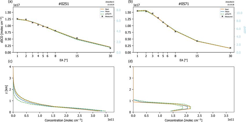
1790                                                                                                       S. Beirle et al.: MAPA

Table 1. Default values for the Monte Carlo-based inversion algo-   is usually accounted for by applying an empirical SF f of
rithm for MAPA v0.98.                                               about 0.8 to the O4 dSCDs for reasons still not understood,
                                                                    while other studies (e.g. Ortega et al., 2016) do not see a need
                   Variable     Default                             for a SF. An in-depth discussion of the O4 SF is provided in
                   β            1                                   Wagner et al. (2018).
                   a            50                                     MAPA provides the option for defining a fixed a priori
                   d            3 (aer)                             scaling factor f of 0.8, for example. Note that within MAPA,
                                2 (tg)                              the measured dSCD is unchanged (in order to have the same
                   ntot = a d   125 000 (aer)                       measured dSCD in plots and result files for comparison), but
                                2500 (tg)
                                                                    the modeled dSCD is divided by f instead.
                   nsel         100
                   F            1.3
                                                                       Another option arises from the profile inversion procedure:
                   caer range   [0.0, 5.0]                          the linear fit of the best matching VCD (Eq. 11), used for the
                   h range      [0.02, 5.0] km                      determination of ctg , can likewise be used to determine the
                   s range      [0.2, 1.8]                          best matching VCD of O4 . This defines the best matching SF
                                                                    as

                                                                    fbm = Va priori /Vbm .                                     (12)
  – absolute minimum and maximum.
                                                                    Note that extreme deviations of f from 1 are flagged later
   The mean profiles are often smeared out; in particular
                                                                    (see Sect. 2.8).
strong vertical gradients (occurring for s ≥ 1) are smeared.
                                                                       As the issue of the O4 SF is still not understood and its
The degree of smearing depends on the variability of param-
                                                                    value or even its need is highly debated within the commu-
eters within the ensemble, which is determined by Rbm and
                                                                    nity, it was decided to always run MAPA with three different
the a priori threshold for accepted RMS values F .
                                                                    settings for f within the FRM4DOAS project:
   Note that mean ± standard deviation might exceed phys-
ical limits for parameters and profiles, similar to LMA fit           1. no scaling of O4 dSCDs, i.e., f ≡ 1,
results ± CI. The 25th and 75th percentiles avoid this. Only
for ctg , which is not determined by a MC approach but by             2. a SF of f = 0.8,
a linear fit, can unphysical (negative) VCDs and concentra-
                                                                      3. a variable (best matching) SF fbm .
tions occur. These can be understood as noise for quasi-zero
VCDs and must not be set to 0 or skipped in order to keep           This setup has also been adopted as default in MAPA v0.98.
unbiased means.                                                     The comparison of the MAPA results for the different set-
   Below we mainly focus on the best match and weighted             tings for f for different campaigns, instruments, and condi-
mean of parameters and profiles.                                    tions will hopefully help to clarify the SF issue in the future.
   Within trace gas retrievals, aerosol profile parameters are
required for accessing the dAMF LUT. For this, the best             2.8   Flags
matching parameters are taken. Due to nonlinearities (the
mean of ensemble profiles does not equal the profile corre-         The profile inversion scheme as described in Sect. 2.6 just
sponding to the mean parameters), it is not possible to use         searches for the parameter combinations yielding best agree-
mean parameters for this. If one is interested in the actual        ment in terms of the lowest R. Thus, it will always result in
aerosol profile and its uncertainty, however, the mean profile      a best match, even if the agreement between measured and
and the percentiles might still yield valuable information.         modeled dSCDs is actually poor, or the resulting parame-
   Figure 2 exemplarily displays O4 dSCDs (top) and the re-         ter ensembles are inconsistent. Therefore, additional infor-
trieved aerosol extinction profiles (bottom) for an afternoon       mation is needed in order to evaluate whether the resulting
sequence on 15 (left) and 23 (right) September 2016. The            profile is trustable or not.
best match, weighted mean, and 25th and 75th percentiles               Within MAPA, flags raising warnings or errors are pro-
are shown. For these examples, a scaling factor of 0.8 has          vided based on the performance of the profile inversion. Note
been applied for O4 (see the next section). This choice will        that output is generated for each elevation sequence, also for
be justified in Sect. 3.                                            those flagged by an error, and the final decision on which pro-
   Figure 3 displays the respective dSCDs and profiles for          files are considered to be meaningful is the user’s. Neverthe-
NO2 .                                                               less, we strongly recommend considering the raised warnings
                                                                    and errors; error flags should generally lead to a rejection of
2.7    Scaling of O4 dSCDs                                          the affected profiles.
                                                                       In this section we describe the warning and error flag crite-
Some previous studies have reported on a significant mis-           ria and thresholds for MAPA v0.98. The thresholds, denoted
match between modeled and measured dSCDs of O4 , which              by 2 below, are defined in the flag configuration file and

Atmos. Meas. Tech., 12, 1785–1806, 2019                                               www.atmos-meas-tech.net/12/1785/2019/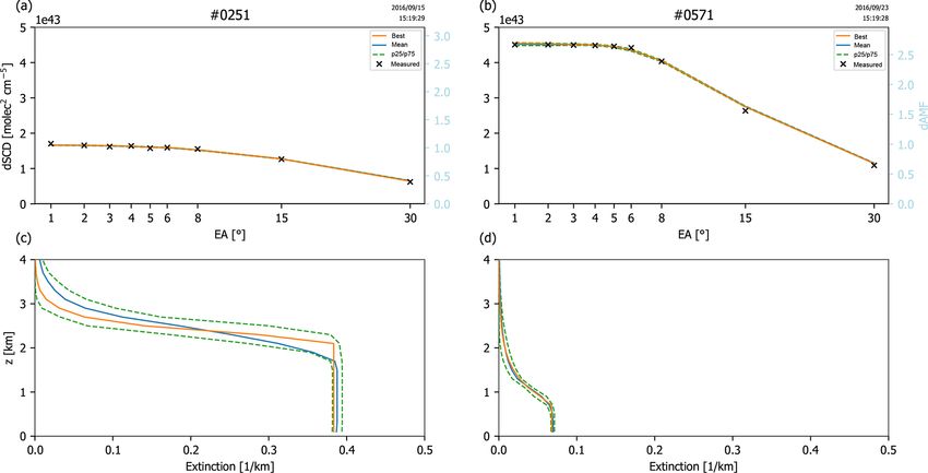
S. Beirle et al.: MAPA                                                                                                                    1791

Figure 2. Illustration of the profile inversion for dSCD sequences of O4 from 15 September (a, c) and 23 September (b, d) 2016. A scaling
factor of 0.8 has been applied (see Sect. 2.7). (a, b) Measured and modeled dSCDs. The parameter ensembles are represented by statistical
key quantities. The right axis (light blue) refers to the corresponding dAMFs. (c, d) Corresponding vertical profiles. Note that the percentiles
of vertical profiles are calculated independently for each height level. That is, they do not correspond to an actual profile from the ensemble
but indicate the general level of uncertainty of vertical profiles.

Figure 3. Illustration of the profile inversion for dSCD sequences of NO2 from 15 September (a, c) and 23 September (b, d) 2016, based
on the aerosol retrievals shown in Fig. 2. (a, b) Measured and modeled dSCDs. The parameter ensembles are represented by statistical key
quantities. (c, d) Corresponding vertical profiles.

www.atmos-meas-tech.net/12/1785/2019/                                                         Atmos. Meas. Tech., 12, 1785–1806, 2019

1792                                                                                                            S. Beirle et al.: MAPA

Table 2. Warning and error threshold default values for MAPA            is given in units of the typical (sequence median) DOAS fit
v0.98. The meaning of the thresholds is explained in the text. The      error Serr .
default column uncertainty ε is 0.05 for aerosols and Verr for trace       Since S scales with the actual VCD V and the dAMF A,
gases.                                                                  R is generally large for high trace gas columns and/or high
                                                                        dAMFs. The first corresponds to polluted episodes, while the
 Symbol     Description                       Warning      Error        second represents conditions under which the MAX-DOAS
 2R         Upper threshold for R             1            3            technique is particularly sensitive. Both cases are of particu-
            in units of Serr                                            lar interest, but would often be flagged if just a threshold for
 2Rn        Upper threshold Rnorm             0.05         0.3          R based on typical values is defined.
 2rel       Relative column tolerance         0.2          0.5
 2abs       Absolute column tolerance         1            4
                                                                           Thus we also consider the RMS normalized by the maxi-
            in units of ε                                               mum dSCD Smax :
 2DL        Column detection limit            1            4
            in units of ε                                               Rn = R/Smax .                                                (13)
 2τ         Upper threshold for AOD           2            3
 2h         Upper threshold for h             3 km         4.5 km       Due to the normalization, Rn removes the scaling of R with
 2LT        Lower threshold for               0.8          0.5          V and A. However, for very low V or A, i.e., dSCDs of about
            LT fraction of total column                                 0, Rn can become quite large and the intrinsic noise of the
 2ϕ         Lower threshold for RAA           15           nan
 2ϕ,τ       Lower threshold for AOD           0.5          3
                                                                        dAMF LUT (if calculated by a MC RTM such as McArtim)
            in order to raise RAA flag                                  matters.
 2f         O4 SF threshold interval          [0.6, 1.2]   [0.4, 1.4]      Warning and errors thus only arise if the values for R and
            (only affects variable SF mode)                             Rn both exceed the thresholds given in Table 2.

                                                                        2.8.2   Consistency
can easily be modified. However, any change should only be
                                                                        In addition to the best matching parameters, MAPA derives
made for good reasons and has to be tested carefully.
                                                                        an ensemble of parameter sets yielding similar agreement in
   Within the FRM4DOAS processing chain, MAPA has to
                                                                        terms of R. But this does not mean that the ensemble pa-
provide reasonable output for a wide variety of instruments
                                                                        rameters are consistent. While different height and shape pa-
and measurement conditions, which could not all be tested
                                                                        rameters might be acceptable (and just result in a larger pro-
beforehand. Thus, the general strategy is to have low thresh-
                                                                        file uncertainty), the column parameter is an important in-
olds for warnings (conservative approach) and higher thresh-
                                                                        tegrated property of the profile. Thus a consistency flag is
olds for errors, indicating cases which do not make sense at
                                                                        defined based on the spread of the column parameter within
all.
                                                                        the ensemble.
   The flags defined in MAPA v0.98 can be grouped into four
                                                                           In order to evaluate if the spread is acceptable or not, we
categories:
                                                                        define ε as a proxy of the column uncertainty. For aerosols,
  1. flags based on the agreement between forward-modeled               ε is defined in absolute terms in the MAPA flag configura-
     and measured S,                                                    tion (default: 0.05). For trace gases, ε is set to Verr , which is
                                                                        derived from the SCD error S err provided in the input data
  2. flags based on consistency of the ensemble of derived              according to Eq. (11).
     MC parameters,                                                        Based on ε, we define the tolerated deviation for c as
  3. flags based on the profile shape, and                              ctol = 2abs × ε + 2rel × cbm ,                               (14)
  4. miscellaneous.                                                     consisting of an absolute term and a relative term. That is,
The different flag criteria are explained in detail below. The          for low columns, the tolerance is dominated by ε scaled with
default warning and error thresholds for MAPA v0.98 are                 the absolute threshold defined in the flag settings, whereas
listed in Table 2.                                                      for high columns, the relative term 2rel × cbm dominates.
                                                                           Flags are raised if the ensemble standard deviation of c
2.8.1   RMS                                                             or the difference between cbm and cwm exceeds the column
                                                                        tolerance.
The RMS R as defined in Eq. (10) reflects the agreement be-                The consistency flag indicates that the observations have
tween measured and best matching S. Thus R might directly               been reproduced with comparable RMS by parameter sets
be used for flagging, as high RMS values generally indicate             with considerably different column parameters. That is, the
that the forward model is not capable of reproducing the mea-           dSCD sequence shows no strong dependency on c, and
surement. In order to account for the instrument-dependent              MAX-DOAS measurements are thus not sensitive for c under
uncertainty of the measured dSCDs, the flag threshold 2R                these conditions.

Atmos. Meas. Tech., 12, 1785–1806, 2019                                                    www.atmos-meas-tech.net/12/1785/2019/
S. Beirle et al.: MAPA 1793
2.8.3 Profile shape
MAX-DOAS measurements are sensitive to the lower tro-
posphere up to about 2–3 km (Frieß et al., 2006). Profiles
reaching up in the free troposphere thus have to be treated
with care. Within MAPA v0.98, these cases are identified and
flagged based on two quantities:
– the fitted height parameter h, and Figure 4. Frequency of cloud conditions as classified based on the
procedure described in Wagner et al. (2016) with adjusted thresh-
– the integrated profile within the lower troposphere cLT
olds for CINDI-2. Missing cloud information is related to missing
(default: below 4 km). O4 dSCDs for single elevation angles. (a) All available elevation
A flag is raised if h > 2h or cLT /cbm < 2LT only if the col- sequences. (b) Only sequences in which AERONET measurements
are available.
umn cbm also exceeds the column detection limit
cDL = 2DL × ε (15)
since for very low columns, the profile shape cannot be spec- 2.8.5 Cloud flag
ified anyhow. Note that per default 2abs equals 2DL ; thus
cDL is the same as the absolute tolerance term in Eq. (14), but Several studies have characterized cloud conditions based on
MAPA also allows us to have different thresholds for both. MAX-DOAS elevation sequences, making use of radiance
and color index and their (inter- and intra-sequence) variabil-
2.8.4 Miscellaneous ity (Gielen et al., 2014; Wagner et al., 2014, 2016; Wang et
al., 2015). While dedicated algorithms have been optimized
In addition, the following flags are defined. for specific instruments, it is difficult to automatize these al-
gorithms as MAX-DOAS instruments are usually not radio-
– Missing elevation angles. In the case of incomplete el-
metrically calibrated; i.e., the thresholds for cloud classifica-
evation sequences, an error is raised during the MAPA
tion have to be adjusted for each instrument.
preprocessing. As profile inversion determines two to
Therefore, no automatized cloud flagging algorithm has
three parameters for about 2–4 degrees of freedom
been included within MAPA so far. However, MAPA pro-
(Frieß et al., 2006), the number M of available EAs
vides the option to add external cloud flags to the MAPA in-
must not be too small; otherwise (default: M < 5) an er-
put. A priori flags in input data are treated like the other flags
ror is raised. Note that for the results for CINDI-2 shown
during MAPA processing, included in the calculation of the
in the following sections, all incomplete sequences are
total flag (see below), and written to the MAPA output. Sim-
removed first, as this is related to missing input data, not
ilarly, other external flags (like an “instrument failure flag”
to the MAPA performance.
etc.) can also easily be added to the MAPA flagging scheme.
– NaNs. Best match, mean, and standard deviation (SD) We have derived a cloud classification based on the
of c are checked for NaNs. These might occur if NaNs scheme described in Wagner et al. (2016), with thresholds
are present in the input data. NaN values automatically adjusted for CINDI-2. Note that cloud information is missing
raise an error. for some elevation sequences due to missing O4 dSCDs for
single elevation angles. Figure 4 displays the classification
– AOD. High AOD likely indicates the presence of clouds. of clouds during CINDI-2 for all elevation sequences as well
But even in the case of cloud-free conditions, high AOD as for those sequences in which AERONET AOD measure-
indicates complex radiative transfer conditions. Thus ments are available. During the campaign, 33 % of the se-
flags are raised if caer ≡ τ > 2τ . quences are categorized as cloud free. If only sequences with
– RAA. If the relative azimuth angle is too low (ϕ < 2ϕ ), coincident AERONET measurements are considered, 72 %
i.e., the instrument is directed towards the sun, and the are cloud free, and the remaining cases are equal parts cloud
AOD is high enough (caer ≡ τ > 2ϕ,τ ), a warning flag hole conditions or missing cloud information. Only 2 % are
is raised. For this scenario, the forward peak of aerosol characterized as broken cloud, and no sequence is character-
scattering matters, which is only roughly captured by ized as continuous cloud. Thus, a comparison of MAPA re-
the Henyey–Greenstein parameterization used in RTM. sults to AERONET to a large extent implies a cloud filtering
even if no dedicated cloud flag is available.
– O4 scaling factor. MAPA provides the option to derive In this study, we do not include the cloud classification in
a best matching SF for O4 (see Sect. 2.7). Large de- the MAPA flagging scheme, as it is not part of the MAPA.
viations of the SF from 1 are flagged according to the Instead, we use the external cloud classification in order to
thresholds defined in Table 2. investigate how far MAPA flags and results for aerosol re-
www.atmos-meas-tech.net/12/1785/2019/ Atmos. Meas. Tech., 12, 1785–1806, 20191794 S. Beirle et al.: MAPA
trieval depend on cloud conditions and how far the current references therein). We thus perform another MAPA retrieval
MAPA flags are able to catch clouded conditions in Sect. 4.5. with an O4 SF of f = 0.8 (Fig. 6).
The application of a SF largely improves MAPA perfor-
2.8.6 Total flag mance and the agreement with AERONET. A far higher
number of sequences is now categorized as valid. The tempo-
As a final step in the flagging procedure, a total warning or ral pattern of AOD generally matches well between MAPA
error flag is raised if any of the flags defined above indicate a and AERONET: correlation is as good as r = 0.874 with a
warning or an error, respectively. mean deviation of 0.012 ± 0.067.
Figure 7 displays MAPA results based on a variable SF.
They are overall similar to the results for a fixed SF of 0.8.
3 Results For the complete campaign, mean and SD of the best match-
ing SF in variable mode are 0.85 ± 0.08.
In this section we present MAPA results exemplarily for
Having the option of a variable (best matching) scaling
dSCD sequences of O4 , NO2 , and HCHO measured dur-
factor is a new feature of MAPA, to our knowledge not pro-
ing the Second Cabauw Intercomparison of Nitrogen Diox-
vided by any other MAX-DOAS inversion scheme. However,
ide Measuring Instruments (CINDI-2) during September
this additional degree of freedom adds complexity, and dif-
2016 (Kreher et al., 2019). We focus on two days, 15 and
ferent effects (like aerosol properties being different from the
23 September, which are mostly cloud free and have also
RTM a priori, or cloud effects) might be “tuned” to an ac-
been selected as reference days within CINDI-2 intercompar-
ceptable match via the scaling factor. As the variable scaling
isons (Tirpitz et al., 2019). The required O4 VCD is derived
factor has not yet been tested extensively, we focus on the
from ECMWF interim temperature and pressure profiles, in-
results for a fixed SF of 0.8 as a more “familiar” and trans-
terpolated in space and time.
parent setup below, but we plan to systematically investigate
For details on the MPIC MAX-DOAS instrument and
the results of best matching SFs for various locations and
DOAS fit settings see Kreher et al. (2019).
measurement conditions in the near future.
3.1 Aerosols
3.2 Nitrogen dioxide (NO2 )
O4 dSCDs have been analyzed according to the DOAS set-
tings specified in Table A3 in Kreher et al. (2019) but with
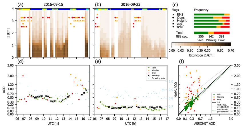
sequential instead of noon reference spectra. Figure 5 dis- The MPIC DOAS retrieval for NO2 has been performed in
plays the MAPA results based on the original O4 dSCD se- a fit window slightly different from that of O4 , i.e., 352 to
quences. In Fig. 5a and b, the valid vertical extinction pro- 387 nm. Figure 8 displays MAPA results for NO2 . The bot-
files are displayed for the two selected days. The invalid tom row now displays the mixing ratio in the lowest 200 m
sequences are marked by the respective flags (symbols as layer instead of the total column. For comparison, mixing ra-
in Fig. 5c). In Fig. 5d and e, the respective time series of tios derived from long-path (LP) DOAS measurements are
AOD are shown and compared to AERONET measurements shown. The LP measurements have been provided by Ste-
(Dubovik and King, 2000)6 . In Fig. 5c, flag statistics are pro- fan Schmitt (IUP Heidelberg). Details on LP instruments and
vided for all available measurements during the campaign, retrieval are given in Pöhler et al. (2010) and Nasse et al.
covering the period from 9 September to 2 October 2016. (2019).
Figure 5f displays a scatter plot of MAPA AOD compared to NO2 profiles are generally far closer to the ground com-
15 min AERONET means where available for the full cam- pared to aerosol profiles, which is expected, as sources are
paign. Note that the scales are not linear in order to cover located at the ground and the NOx lifetime of some hours is
the different order of magnitude in AOD for the two selected far shorter than that of aerosols.
days. Comparison of the NO2 mixing ratio in the lowest 200 m
A large fraction of sequences are flagged (overall, less than layer to LP measurements yields a correlation of r = 0.887.
one-fourth of all sequences are valid). On 23 September, not The mean difference between MAPA and LP mixing ratios
a single valid sequence was found from 09:00 to 14:00 UTC. for valid sequences is 0.84 ± 2.26 ppb.
Even worse, the remaining AODs do not match AERONET The flagging is strongly dominated by the aerosol flag in-
(e.g. afternoon of 23 September). herited from the aerosol analysis.
This poor performance is related to a general mismatch be-
tween modeled and measured dSCDs, as has also been found 3.3 Formaldehyde (HCHO)
for other campaigns in the past (see Wagner et al., 2018, and
6 The original level 2 AERONET AOD determined at 440 nm has HCHO dSCDs have been analyzed according to the DOAS
been transferred to 360 nm by assuming an Ångström exponent of settings specified in Table A4 in Kreher et al. (2019) but with
1. a sequential instead of a noon reference spectrum.
Atmos. Meas. Tech., 12, 1785–1806, 2019 www.atmos-meas-tech.net/12/1785/2019/S. Beirle et al.: MAPA 1795
Figure 5. MAPA results for aerosols during CINDI-2. (a) Vertical extinction profile on 15 September. Gaps are flagged as warning (orange)
or error (red), indicated by different symbols for the different flag criteria. Results of the cloud classification are provided at the top (for
details see Sect. 2.8.5; colors as in Fig. 4). Panel (b) is as (a) but for 23 September. (c) Flag statistics for the whole CINDI-2 campaign.
(d) AOD from MAPA compared to AERONET for 15 September. Panel (e) is as (d) but for 23 September. (f) MAPA AOD compared to
AERONET for the whole CINDI-2 campaign.
Figure 9 displays MAPA results for HCHO. Profiles reach settings and the impact on the number of valid sequences and
up higher than for NO2 as expected due to HCHO being a the resulting AOD, compared to AERONET. It also includes
secondary product in VOC oxidation. results for a previous MAPA version as well as for different
As for NO2 , the flagging is dominated by the aerosol flag. O4 SFs, as discussed in Sect. 4.3 and 4.4.
But in addition, several more sequences are flagged, with Finally, Sect. 4.5 investigates the dependency of MAPA
contributions from all RMS, consistency, and profile shape flag statistics on cloud conditions.
flags.
Comparison of the HCHO mixing ratio in the lowest 200 m 4.1 MC settings
layer to LP measurements yields a correlation of r = 0.937.
The mean difference between MAPA and LP mixing ratios In this section, the MC settings as defined in the MAPA MC
for valid sequences is 0.35 ± 0.56 ppb. configuration file are modified one by one.
A. Random seed. The random generator can be initialized
by the seed β provided in MAPA MC configuration.
4 Sensitivity studies This allows us to generate reproducible results even
though the method is based on random numbers. We
The MAPA profile inversion and flagging algorithms are con- have tested two alternative seed values just to check how
trolled by a priori parameters. These have been defined by strong the impact of usage of random numbers is. The
plausible assumptions. In this section we investigate how number of valid sequences and the results for AOD only
sensitive the MAPA results are for different a priori settings, change slightly for different random sets.
based on the aerosol retrieval for CINDI-2 applying a fixed
SF of 0.8 and its comparison to AERONET. B. Number of random samples. As default, each profile pa-
In Sect. 4.1, the sensitivity to MC settings is investigated. rameter is sampled by a = 50 values per variable. That
The impact of flagging thresholds is analyzed in Sect. 4.2. is, for the height parameter, which is within 0.02 and
Note that flag settings can easily be modified a posteriori, 5 km, the average spacing of the raster in the h dimen-
while different MC settings require a complete reanalysis. sion is about 0.01 km (note that the average spacing be-
Table 3 lists the investigated variations for both MC and flag comes smaller in the second and third iterations of the
www.atmos-meas-tech.net/12/1785/2019/ Atmos. Meas. Tech., 12, 1785–1806, 20191796 S. Beirle et al.: MAPA Figure 6. As Fig. 5 but for a SF of 0.8. Figure 7. As Fig. 5 but for a variable (best matching) SF. The resulting SFs are shown in light blue in panels (d) and (e) (for scale see right axis of e). Atmos. Meas. Tech., 12, 1785–1806, 2019 www.atmos-meas-tech.net/12/1785/2019/
S. Beirle et al.: MAPA                                                                                                           1797

Figure 8. MAPA results for NO2 during CINDI-2, based on aerosol profiles retrieved with a SF of 0.8. (a) Vertical concentration profile
on 15 September. Panel (b) is as (a) but for 23 September. (c) Flag statistics for the whole CINDI-2 campaign. (d) Mixing ratio in the
lowest layer (0–200 m above ground) from MAPA compared to long-path (LP) DOAS results for 15 September. Panel (e) is as (d) but for 23
September. (f) MAPA lowest layer mixing ratio compared to LP for the whole CINDI-2 campaign.

Figure 9. As in Fig. 8 but for HCHO.

www.atmos-meas-tech.net/12/1785/2019/                                                   Atmos. Meas. Tech., 12, 1785–1806, 2019
1798                                                                                                                 S. Beirle et al.: MAPA

Table 3. Variations of a priori settings (compared to the default) and their impact on the MAPA aerosol retrieval, quantified by the number of
valid sequences and the AOD comparison between MAPA and AERONET (correlation coefficient r and difference 1τ ). The default settings
of MAPA v0.98 with a SF of f = 0.8 are considered baseline. Variations A–D refer to settings of the MC algorithm (Sect. 4.1). Variations
a–e refer to flag thresholds (Sect. 4.2). Results for a previous MAPA release and results for different SFs are included as well. For details and
discussion see the text.

                                Setup         Variation               No. of valid       r                   1τ
                                              (default)                sequences
                                f = 0.8       –                            324        0.874      0.012 ± 0.067
                                A1            β = 2 (1)                    320        0.882      0.014 ± 0.070
                                A2            β = 1000 (1)                 329        0.876      0.014 ± 0.069
                                B1            a = 20 (50)                  269        0.882      0.014 ± 0.076
                                B2            a = 100 (50)                 342        0.860      0.026 ± 0.088
                                C1            F = 1.1 (1.3)                389        0.872      0.026 ± 0.072
                                C2            F = 1.5 (1.3)                279        0.908      0.006 ± 0.058
                                D1            smin = 0.1 (0.2)             311        0.875      0.019 ± 0.071
                                D2            smin = 0.5 (0.2)             348        0.848      0.004 ± 0.073
                                D3            smax = 1.5 (1.8)             330        0.887      0.018 ± 0.067
                                a1            2R = 0.5 (1)                 324        0.874      0.012 ± 0.067
                                a2            2R = 2 (1)                   325        0.874      0.012 ± 0.067
                                a3            2Rn = 0.025 (0.05)           238        0.911      0.022 ± 0.064
                                a4            2Rn = 0.1 (0.05)             338        0.874      0.012 ± 0.067
                                b1            ετ = 0.025 (0.05)            311        0.877      0.011 ± 0.067
                                b2            ετ = 0.1 (0.05)              334        0.876      0.014 ± 0.068
                                c1            2rel = 0.1 (0.2)             299        0.894      0.006 ± 0.054
                                c2            2rel = 0.4 (0.2)             340        0.787      0.022 ± 0.094
                                c3            2abs = 0.5 (1)               311        0.877      0.011 ± 0.067
                                c4            2abs = 2 (1)                 334        0.876      0.014 ± 0.068
                                d1            2h = 2 (3) km                307        0.916      0.003 ± 0.055
                                d2            2h = 4 (3) km                338        0.783      0.032 ± 0.124
                                e1            2τ = 1 (2)                   323        0.874      0.012 ± 0.067
                                e2            2τ = 3 (2)                   327        0.874      0.012 ± 0.067
                                v0.96                                      337        0.826      0.037 ± 0.126
                                f = 1.0       –                            218        0.905     −0.115 ± 0.043
                                Variable f    –                            356        0.873     −0.018 ± 0.069

     narrowed parameter intervals; see Sect. 2.6.2). The total                   more homogeneous, and fewer sequences are flagged as
     number of random parameter sets ntot is a to the power                      inconsistent.
     of MC variables, i.e., 503 = 125 000 for aerosols. This                     We found a = 50 to be a good compromise between
     corresponds to a duration of about 3 s per elevation se-                    computation time and the number of valid sequences.
     quence on a normal PC.
                                                                             C. Ensemble threshold for RMS. MAPA determines the
     If a is lowered to 20 (ntot = 8000), the profile inver-                    best matching parameter combination by the lowest
     sion is much faster. But only 269 instead of 324 se-                       RMS R. In addition, an ensemble of parameter sets is
     quences are identified as valid. However, the remain-                      kept with R < F × Rmin . The resulting ensemble allows
     ing profiles show good agreement with AERONET. If                          us to estimate the uncertainty of the derived parameters
     a number of a = 100 (ntot = 106 ) is chosen, about 20                      and profiles. Per default, F is set to 1.3. We have tested
     more sequences are labeled as valid compared to the                        smaller and higher values for F in scenarios C1 and C2.
     baseline. But the agreement with AERONET becomes
                                                                                 For a low value of F = 1.1, a far higher number of
     slightly worse, and the required time is more than 10-
                                                                                 sequences is characterized as valid. This is due to the
     fold.
                                                                                 variety of parameters in the ensemble being lowered,
     The impact of a on the number of valid sequences can                        and consequently the consistency thresholds are less of-
     be understood as for higher a, the parameter space is                       ten exceeded. Another side effect is that the profile un-
     sampled at a finer resolution. Thus the RMS of the best                     certainty estimate, which is derived from the variabil-
     match, Rbm , generally becomes lower. Consequently,                         ity of profile parameters, is also lowered. For the ex-
     the parameter ensemble defined by R < F × Rbm is                            treme scenario FR → 1, only the best matching param-

Atmos. Meas. Tech., 12, 1785–1806, 2019                                                        www.atmos-meas-tech.net/12/1785/2019/
S. Beirle et al.: MAPA 1799
eter set would be left, which would be close to the re- Per default, ετ is set to 0.05. A lower or higher value
sult from the LMA if the number of randoms is high for ετ slightly decreases or increases the number of
enough. Interestingly, the agreement to AERONET is valid sequences, respectively, but the agreement with
slightly worse for a low F . AERONET hardly changes.
Conversely, a higher value for F results in fewer valid
sequences (as more sequences are characterized as in- c. Consistency. The variations of the thresholds related
consistent), but the remaining ones show better agree- to the consistency flag can be summarized as fol-
ment with AERONET. lows. More strict criteria (c1 and c3) result in fewer
For MAPA v0.98 default settings, we stick to the choice valid sequences but a slightly better agreement with
of F = 1.3. But we recommend also testing smaller val- AERONET. Vice versa, less strict criteria (c2 and c4)
ues for F like 1.2 or 1.1, in particular if a large fraction result in more valid sequences with poorer agreement
of sequences is flagged by the consistency flag. with AERONET. We consider the current default set-
tings to be plausible and a good compromise.
D. Shape parameter limits. The shape parameter s deter-
mines the profile shape according to Sect. 2.4. Modify- d. Profile shape. Here we focus on variations of 2h . The
ing the allowed parameter range thus changes the basic impact of modifications of 2LT (not shown) is similar.
population of possible profile shapes within the random
ensemble. If 2h is set to 4 km, which was the default value in
By default, the shape parameter almost covers the nodes previous MAPA versions (compare Sect. 4.3), more
of the dAMF LUT, except for smin , which is set to 0.2. sequences are labeled as valid, but the agreement to
Changing this to 0.1 means allowing for boxes with AERONET becomes worse. For instance, for the mea-
long exponential tails, which are likely flagged later surements around 16:00 UTC on 15 September, when
by the profile shape flag due to the LT criterium. Set- MAPA AOD is far higher than AERONET, a warning
ting smin = 0.1 worsens the performance (fewer valid was raised by the height parameter (see Fig. 6a and d).
sequences as expected; slightly poorer agreement to For 2h = 4 km, these sequences are labeled as valid.
AERONET), while a value of 0.5 improves the differ- If the threshold 2h is lowered to 2 km, fewer valid
ence but not the correlation to AERONET. sequences remain, but those show significantly bet-
Setting smax to 1.5 (i.e., removing very thin elevated lay- ter agreement with AERONET, for both correlation
ers from the basic population) has almost no effect on and difference. This reflects that MAX-DOAS mea-
the CINDI-2 aerosol results. surements are mainly sensitive for profiles close to the
ground (Frieß et al., 2006). Consequently, inversion re-
4.2 Flag settings sults for profiles reaching up to higher altitudes have
higher uncertainties.
Here we modify the flag settings and thresholds as defined in
the MAPA flag configuration file one by one. Except for the This is also illustrated in Fig. 10, showing the agreement
thresholds for height parameter and AOD, the default values between MAPA and AERONET AOD as a function of
are halved and doubled. the height parameter h.
a. RMS. We have changed the RMS thresholds for R and
Rn in both directions. A change in the threshold of R e. AOD. Modifications of the AOD threshold have almost
has hardly any effect in the case of our CINDI-2 results. no effect. This might however be different for measure-
This might of course be different for other instruments ments under a higher aerosol load.
or measurement conditions.
Lowering the threshold for Rn has a tremendous effect: 4.3 MAPA version 0.96
86 more sequences would be flagged compared to the
default. The remaining sequences show a better corre- In Table 3, the results for previous MAPA version 0.96 are
lation, but slightly worse agreement with AERONET also included. This version was used for the FRM4DOAS
AOD. Increasing 2Rn has only a small effect, as most verification study (Richter and Tirpitz, 2019).
sequences with high Rn values are already flagged by Version 0.96 was based on the same MC algorithm with
one of the other criteria. the same MC settings as v0.98. However, the flag definitions
and thresholds differ slightly. The main difference is that the
b. Column uncertainty proxy. For trace gases, εtg can be height threshold for the profile shape flag was set to 4 km in
determined from the dSCD sequence (see Sect. 2.6.1). v0.96. Consequently, v0.96 results in more valid sequences
This is not possible for the aerosol retrieval. Instead, ετ but with slightly poorer agreement with AERONET AOD,
has to be defined by the user. similar to variation d2.
www.atmos-meas-tech.net/12/1785/2019/ Atmos. Meas. Tech., 12, 1785–1806, 20191800 S. Beirle et al.: MAPA
Figure 10. Dependency of the ratio of AOD from MAPA
vs. AERONET as a function of the height parameter h. Color in-
dicates MAPA flags.
4.4 Different scaling factors
The results presented above are based on an O4 SF of 0.8. If
instead no scaling factor is applied, a far higher number of
sequences is flagged, and only 218 sequences remain. These
show a good correlation to AERONET but a systematic bias
of −0.115 (compare Fig. 5). The ratio of the mean AOD from
MAPA vs. AERONET is 0.53; i.e., MAPA results are too low
by a factor of 2 on average if no SF is applied.
If the SF is considered to be variable, about 30 more se-
quences are valid, with similar agreement to AERONET as
for a fixed SF of 0.8.
4.5 Clouds
Figure 11 displays the MAPA flag statistics in dependency
of cloud conditions (Sect. 2.8.5) during CINDI-2. For the
full campaign, 36 % of all sequences are valid. If only cloud-
free scenes with low aerosol are considered, 68 % are valid, Figure 11. Statistics of MAPA flags for different cloud conditions.
while for clouded scenes (broken + continuous clouds), only
13 % are valid. Note that the flags for RMS, consistency,
height, and AOD all contribute significantly to the flagging other datasets. We start with issues generally affecting MAX-
of clouded scenes. DOAS inversions, followed by MAPA-specific issues.
For the selection of sequences in which AERONET is
available, 65 % sequences are valid. 5.1 General limitations of MAX-DOAS profile
For CINDI-2, most clouded cases are successfully flagged inversions
in MAPA. But a significant number of cloud hole/broken
cloud scenes still remain. We thus recommend that the user In this section we discuss general MAX-DOAS limitations,
applies an additional cloud classification according to Wag- which also account for optimal estimation algorithms. Still,
ner et al. (2016), for example, and flag cloud holes with a the issues are discussed from a MAPA perspective.
warning and continuous and broken cloud scenes with an er-
ror. 5.1.1 RTM assumptions
Within forward models, RTM calculations are required,
5 Limitations which need a priori information such as aerosol properties.
If this information is not available and wrong assumptions
In this section we discuss challenges and limitations of are made, resulting profiles are biased.
MAX-DOAS profile inversion, which have to be kept in For MAPA, the dAMF LUT used in the forward model has
mind when interpreting the results and comparing them to been calculated based on a priori assumptions as specified in
Atmos. Meas. Tech., 12, 1785–1806, 2019 www.atmos-meas-tech.net/12/1785/2019/You can also read