Electromagnetically induced transparency based Rydberg-atom sensor for quantum voltage measurementsa
←
→
Page content transcription
If your browser does not render page correctly, please read the page content below
Electromagnetically induced transparency based Rydberg-atom sensor for
                                                   quantum voltage measurementsa)
                                                             Christopher L. Holloway,1 Nikunjkumar Prajapati,1, 2 John Kitching,1 Jeffery A. Sherman,1 Carson Teale,1 Alain
                                                             Rüfenacht,1 Alexandra B. Artusio-Glimpse,1 Matthew T. Simons,1 Amy K. Robinson,3 and Eric B. Norrgard4
                                                             1)
                                                                National Institute of Standards and Technology, Boulder, CO 80305, USAb)
                                                             2)
                                                                Department of Physics, University of Colorado, Boulder, CO 80305, USA
                                                             3)
                                                                Department of Electrical Engineering, University of Colorado, Boulder, CO 80305,
                                                             USA
                                                             4)
                                                                National Institute of Standards and Technology, Gaithersburg, Maryland 20899,
                                                             USA
                                                             (Dated: 26 October 2021)
arXiv:2110.02335v2 [physics.atom-ph] 22 Oct 2021

                                                             We investigate the Stark shift in Rydberg rubidium atoms through electromagnetically induced transparency
                                                             for the measurement of direct current (dc) and 60 Hz alternating current (ac) voltages. This technique
                                                             has direct applications to atom-based measurements of dc and ac voltage and the calibration of voltage
                                                             instrumentation. We present experimental results for different atomic states that allow for dc and ac voltage
                                                             measurements ranging from 0 V to 12 V. A Rydberg atom-based voltage standard could become an alternative
                                                             calibration method with more favorable size, weight, power consumption, and cost compared to the more
                                                             precise Josephson voltage standard. In this study, we also demonstrate how the voltage measurements can
                                                             be utilized to determine the atomic polarizability for the Rydberg states. The Rydberg atom-based voltage
                                                             measurement technology would become a complimentary method for dissemination of the voltage scale directly
                                                             to the end user.

                                                   I.   INTRODUCTION

                                                      Rydberg atoms (atoms with one or more electrons
                                                   excited to a very high principal quantum number n1 )
                                                   in conjunction with electromagnetically-induced trans-
                                                   parency (EIT) techniques have been used to success-
                                                   fully detect and fully characterize radio frequency (RF)
                                                   electric (E) fields2–6 . In these applications, the E-fields
                                                   are detected using EIT both on resonance as Autler-
                                                   Townes (AT) splitting and off-resonance as ac Stark
                                                   shifts. This approach has the capability of measur-
                                                   ing amplitude3–6,8–11 , polarization12,13 , and phase14,15 of
                                                   the RF field and various applications are beginning to
                                                   emerge. These include E-field probes5,6,10 traceable to
                                                   the International System of units (SI), power-sensors16 ,
                                                   spectrum analyzers17 , angle-of-arrival detection18 , and          FIG. 1. Cylindrical vapor cell with stainless-steel parallel
                                                   receivers for communication signals (AM/FM modulated               plates. The vapor cell is 50 mm in length and has a out-
                                                   and digital phase modulation signals)19–26 .                       side diameter of 25 mm. The plates are rectangular in shape
                                                      In this manuscript, we investigate the use of Rydberg-          with width of 18 mm, length of 45 mm, and placed ≈ 2 mm
                                                   atom sensors to develop a quantum-based voltage stan-              apart.
                                                   dard. Here, we measure the voltage induced between
                                                   two parallel plates embedded in an atomic vapor cell (see
                                                   Fig. 1) by measuring the Stark shifts in the atomic spec-
                                                   tra of Rydberg atoms. By collecting a series of mea-                  The primary voltage standard implemented for the re-
                                                   surements of the Stark shift for different voltages, we can        alization of the SI volt is based on the Josephson ef-
                                                   make a calibration curve and demonstrate a voltage stan-           fect. Arrays of Josephson junctions, when cooled to cryo-
                                                   dard. We discuss various issues that must be considered            genic temperatures and biased on their quantum lock-
                                                   in order for Rydberg-atom-based-sensors to accurately              ing range transduce an accurately synthesized microwave
                                                   and reliably function as voltage measurement standards.            frequency source into fixed or digitally programmable
                                                                                                                      voltages27 . Comparisons between such voltage standards
                                                                                                                      demonstrate accuracies at the level of 1 part in 1010 with
                                                                                                                      about 100 s of averaging (see, e.g.28 ). Scaling up the
                                                   a) Publication of the U.S. government, not subject to U.S. copy-   voltage output of Josephson-junction based standards re-
                                                   right.                                                             quires either increasing the number of junctions in the
                                                   b) Electronic mail: christopher.holloway@nist.gov
                                                                                                                      array, or increasing the microwave driving frequency, or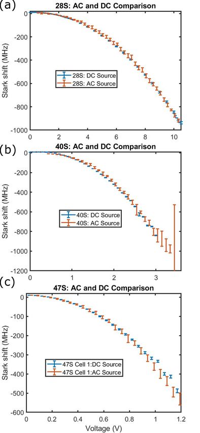
2

both29 . With some exceptions (see, e.g.30 ), 10 V is the       II.   VOLTAGE MEASUREMENTS
commonly adopted dc reference for the primary realiza-
tion of the voltage scale. Commercial instruments (like           A Rydberg atom-based dc (or 60 Hz) voltage measure-
voltage calibrators) used for the routine voltage calibra-      ment is performed by observing the dc (quasi-dc) differ-
tion process and voltage dividers implemented to expand         ential Stark shifts in Rydberg states, which is given by42
the range to high voltages typically have an accuracy on
the order of 1 part in 106 31 . Due to their large cost                                          α(f ) 2
                                                                                        ∆=            E ,                       (1)
(& $300k) Josephson voltage standards limit their de-                                             2
ployment to national metrological institutes (NMIs) or
primary calibration laboratories.                               where ∆ is the Stark shift (in units of Hz), E is the
                                                                applied electric field (in units of V/m) with frequency f
                                                                (in units of Hz), and α(f ) is the polarizability [in units
  Zener diodes are the most commonly used voltage ref-          of Hz/(V2 /m2 )]. For Rydberg state i, the polarizabiltiy
erences that are implemented with commercial instru-            may be expressed as
mentation, ranging from high performance secondary
voltage standard (> $10k)32,33 to the 0.1 % accuracy                          X |µzij |2           1                 1
                                                                  αi (f ) =                                  +                   .
handheld multimeters (≈ $100). All Zener-diode volt-                                h        fij − f − 2i Γj   fij + f + 2i Γj
                                                                               j
age references drift with time and require periodic cali-
                                                                                                                         (2)
bration, that involves a comparison with a more accurate
                                                                Here, the summation includes all states j which are cou-
voltage reference or another verification of the manufac-
                                                                pled to i by electric field, µzij is the z component of the
turer specifications. Zener-diode references are sensitive
                                                                dipole matrix element, fij is the transition frequency, and
to temperature, humidity, mechanical stress and shock,
                                                                Γj is the spontaneous decay rate (in units of Hz) of state
and power supply noise32 .
                                                                j, respectively. Table I gives the calculated dc polariz-
                                                                ability α(0) for the atomic states used in the experiments
   Rydberg atom sensors, that rely on the atom’s pre-           presented in this paper using Eq. (2) and dipole matrix
dictable response to electric field to measure voltage          elements µij taken from the Alkali Rydberg Calculator
could become an alternative — in terms of size, weight,         Python package43 . This package calculates dipole matrix
power and cost (SWaP-C) — to Zener voltage references           elements using the Coulomb approximation (CA) and the
and, with lesser accuracy, to Josephson voltage stan-           quantum defects given in Ref. 44 . Reference45 compared
dards. For example, polarizability measurements with            the accuracy of polarizablities calculated using the CA
low-lying excited states of alkaline-earth atoms show to-       to calculations with the more detailed Dirac-Fock with
tal inaccuracy at the level of 2 parts in 105 34,35 . Due to    core potential approach. For the 28S to 47S Rydberg
a large dipole moment, Rydberg atomic states have high          states considered here, the theoretical polarizability val-
sensitivity to electric fields, high intrinsic response band-   ues calculated using the CA are accurate to better than
width, and can be produced by laser excitation in large         1 %. The accuracy of the theoretical values exceed the
quantities within simple vapor cells at or near room tem-       experimental accuracy for these states, which is typically
perature. In principle, the atomic response can be made         on the level of a few percent46,47 . Because fij  60 Hz,
free from environmental coupling, which would make Ry-          α(f = 60 Hz) ≈ αf (0). To the precision given in Table I
dberg atom sensors intrinsically stable, eliminating the        (< 0.1 %), α is identical for f = 0 and f = 60 Hz.
need of subsequent periodic external calibrations.                 If the E-field is generated by applying a voltage across
                                                                two parallel plates with separation d (neglecting fringing
                                                                field, see discussion in section VI), then the E-field is
   In this paper, we discuss the various nuances of             E = V /d. By substituting this into equation Eq. (1), the
Rydberg-atom-based voltage measurements [e.g., the ef-          voltage can be found by measurement of the Stark shift:
fects of energy level crossing and non-parallel electrodes
(causing inhomogeneous fields)]. While similar measure-
                                                                                              r
                                                                                                  2∆
ments have been performed before38–41 , our study focuses                               V =d           .                 (3)
                                                                                                   α
on the aspects that will need to be addressed and con-
trolled for a Rydberg-atom sensor to be used as a volt-         From this expression, we see that there are three sources
age measurement standard. We also demonstrate two               of uncertainties in this measurement. There are two mea-
methods for measuring ac voltage amplitude at 60 Hz.            sured quantities in this expression (the plate separation
AC Stark effect measurements have been performed in             d and the Stark shift ∆) and one calculated quantity
Ref.38 , where it was shown that indium tin oxide elec-         (the atomic polarizability, α). α can also be determined
trodes where limited to 40 kHz and nickel electrodes op-        experimentally.
erated down to dc. Our cells achieve dc and low fre-               The measurement of ∆ can be related to in situ
quency sensing with stainless steel plates. Finally, we         laser spectroscopy of the hyperfine structure, contribut-
discuss how accurate measurements of the Stark shifts           ing a relative precision of 10−7 or better48 . Relative
and the plate separation can lead to accurate estimates         uncertainty in d of 10−4 is possible with gauge-block
of the polarizability for Rydberg states.                       construction36 or at < 2 × 10⁻⁵ with interferometric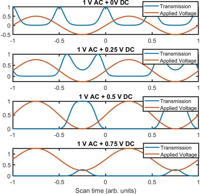
3

                                                                          100 Rb 40S
TABLE I. Theoretical calculation of dc and 60 Hz ac polariz-
abilities for 85 Rb. Note that the dc and 60 Hz ac polarizabil-
ities are essentially the same for the digits shown                         0

                                                                  (MHz)
           Calculated Polarizability [Hz/(V/m)2 ]                         100
            Rydberg state α: dc and 60 Hz ac                              200
                                                                          300
                28S1/2               84.2
                                                                          400
                                                                          100 Rb 40D
                40S1/2              1058.1
                47S1/2              3275.7
                                                                            0

                                                                  (MHz)
                                                                          100
techniques34,35 . Typically, poor knowledge of µij lim-                   200
                                                                                 |mJ| = 1/2
its the calculation of α to the 10−3 level, though in some                300    |mJ| = 3/2
                                                        37                       |mJ| = 5/2
cases α is experimentally determinable by other means
                                                   √       .              4000              100   200         300          400                  500
Even lacking absolute knowledge, the quantity d/ α can                                              E (V/m)
be calibrated to the extent that d remains stable. For a
given device, Equation 3 is cast as:                                                                                85
                                                                  FIG. 2. Calculated dc Stark shift ∆f in                Rb as a function
                                 √                                of electric field E for 40S and 40D.
                        V = Ccal ∆                      (4)
                    √
where Ccal = 2d/ α is determined by comparison to a                (a)                    (b) 780 nm          480 nm
                                                                          nS 1/2
                                                                                              Laser           Laser
higher accuracy voltage standard, or by use of several
                                                                                    480 nm                                              Photo-
Rydberg states with various α of lower uncertainty.                                                                                    detector
   The dc and 60 Hz measurements will share a common                 5P3/2            F'=4
Ccal . Other sources of uncertainty arise from fringing                            780 nm                                         Voltage Voltage
                                                                                                                                 Source Meter
                                                                                                        85
fields near the perimeter of the electrode plates, non-           5S1/2             F=3                  Rb                   02.40V   02.40V

idealities in plate geometry and orientation, and spectro-
scopic features due to interfering transitions.
                                                                  FIG. 3. (a) Level diagram depicting EIT coupling the
                                                                  5S1/2 ,F=3 state to a nS1/2 Rydberg state through the
III.   EXPERIMENTAL SETUP                                         5P3/2 ,F’=4 intermediate state. (b) Experimental setup for
                                                                  the voltage measurement and the three-level EIT scheme.
   In these experiments, we generate EIT in rubidium
(85 Rb) atomic vapor and measure the frequency shift in
the EIT signal as a function of an applied voltage across         Stark spectrum of D states is typically complicated by
two parallel plates. The experimental apparatus is shown          the fine structure, resulting in many more possible en-
in Fig. 1. It consists of a cylindrical-vapor cell of length      ergy level crossings (ELC) than seen in the S states. We
50 mm and diameter of 25 mm. Inside the cell are two              therefore focus on S states as they are typically well de-
stainless-steel parallel plates with a nominal separation         scribed by Eq. 1. However, as we will see below, for large
of d = 2 mm. We had two of the same type of cells man-            applied voltages, ELCs do appear in the S-state spectra
ufactured and we are able to determine that the plate             and can influence the measurements.
separation for the two cells were approximately 2.19 mm              The experimental setup and the atomic levels used are
(referred to as “Cell 1”) and 2.11 mm (referred to as             depicted in Fig. 3, which consists of a 780 nm probe laser,
“Cell 2”), which is within the uncertainty for the plate          a 480 nm coupling laser, a photodetector connected to an
separation stated by the manufacturer. While the data             oscilloscope, a voltage source, a voltage meter, and the
shown in this paper are for Cell 1, we do comment on              vapor cell shown in Fig. 1 filled with 85 Rb atomic vapor.
the data from Cell 2. The plates in both cells are not            We use a three-level EIT scheme to generate Rydberg
perfectly parallel to one another, which causes field in-         atoms [see Fig. 3(a)] which corresponds to the 85 Rb 5S1/2
homogeneities across the plates. We discuss the effect            as the ground state, 5P3/2 as the intermediate state, and
this has on the EIT spectra and voltage measurement in            a Rydberg state of nS1/2 state. In these experiments we
Section VI.                                                       use n = 47, n = 40, and n = 28. The probe laser is locked
   Using a Rydberg-atom EIT measurement scheme for                to the D2 transition (5S1/2 (F = 3) – 5P3/2 (F = 4) or
measuring Stark shifts involves exciting the atoms to             wavelength of λp = 780.24 nm49 ). To produce an EIT
some Rydberg state. States with zero orbital angular mo-          signal, we apply a counter-propagating coupling laser
mentum (S states) exhibit a less complicated spectrum             with λc ≈ 480 nm and scan it across the 5P3/2 -nS1/2 Ry-
as a function of applied electric field. Fig. 2 shows the         dberg transition. We use a lock-in amplifier to enhance
calcualted Stark shift of the 85 Rb 40S1/2 state (Fig. 2a)        the EIT signal-to-noise ratio by modulating the coupling
and 40Dmj state (Fig. 2b). Compared to S states, the              laser amplitude with a 37 kHz square wave. This removes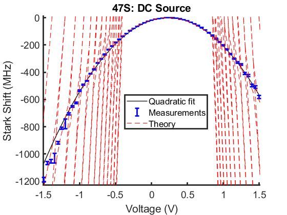
4
the background and isolates the EIT signal.
A voltage source is connected to the electrodes on the
outside of the vapor cell shown in Fig. 1. These electrodes
penetrate the cell and are connected to the two parallel
plates. The EIT signal frequency shift (the Stark shift) is
measured for different applied voltages. The voltage me-
ter is also connected to the electrodes in order to monitor
the applied voltage. Both the voltage sources and volt-
age meter were calibrated before the experiments and
the absolute voltage accuracy of any reading is 0.5 mV.
In these experiments, the optical beams and the electric
fields between the two plates are co-linearly polarized.
The probe laser was focused to a full-width at half max-
imum (FWHM) of 80 µm with a power of 3.6 µW, and
the coupling laser was focused to a FWHM of 110 µm
with a power of 70 mW.
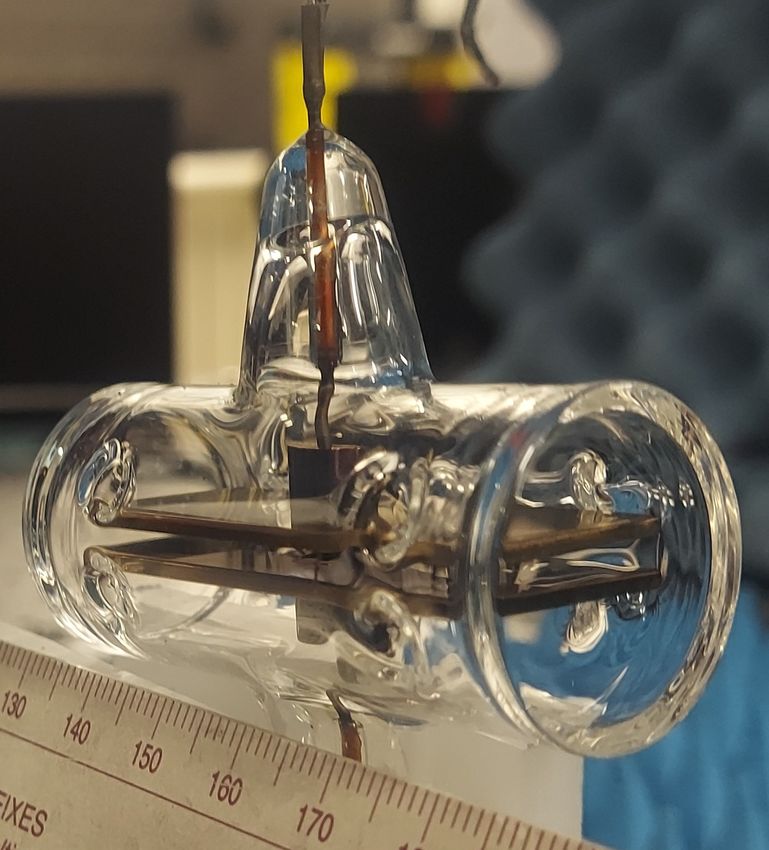
FIG. 4. Plot of % probe EIT transmission relative to the
IV. EXPERIMENTAL DATA probe absorption plotted against the coupling laser detuning.
The black-solid curve is the transmission trace for the 40S
The EIT signals for two different applied voltages are Rydberg state when no voltage is applied across the plates.
shown in Fig. 4. These results are for the 40S1/2 state The red-dashed curve is the transmission trace for the 40S
Rydberg state when a potential of 2.4 V is placed on the
as the coupling laser is scanned. To increase the sig-
plates.
nal to noise ratio, we gather 20 oscilloscope traces and
average them after accounting for laser drift using an
external reference EIT signal. The two different traces
correspond to the zero voltage case (black-solid trace) lines, including additional structure in the EIT signal
and the case with 2.4 V applied (red-dashed trace). For that start to appear. The structure becomes complicated
no applied voltage, we see two peaks, the main EIT peak for higher applied voltages. These structures stem from
at ∆c /2π = 0 MHz and another at ∆c /2π = −75.6 MHz, two sources. First, these structures are due to the ELC
which corresponds to the hyper-fine structure transi- beginning to appear in the spectra. Secondly, the source
tion 5P3/2 (F = 3) → 40S1/2 . Since the coupling laser of these structures (that eventually develops into double
is scanned, the separation between these two peaks is peaks for higher voltages) are a result of inhomogeneities
75.63 MHz. The detuning of the observed peak is the in the field across the laser beam propagation path. The
adjusted hyper-fine splitting determined by accounting inhomogeneities in the field are mainly caused by (1)
for the doppler mismatch between the probe and cou- non-parallel plates, (2) imperfections in the surface of
λ the electrodes due to attaching lead to the plates [as our
pling lasers with 120.96( λpc − 1) MHz. Here, λp and λc
are the wavelengths of the probe and coupling lasers, current plates have a dimple (and discontinuities) in the
and 120.96 MHz is the hyper-fine structure separation very center where the leads are mounted], and (3) fringing
between 5P3/2 (F=3) and 5P3/2 (F=4)49 . The separation fields at the edge of the plates. To confirm the plates are
between the main EIT peak and the peak corresponding not parallel, we used a microscope to measure the plate
to the hyper-fine structure is used to calibrate the laser separation at the four corners. We measured the elec-
detuning and the frequency for the measured Stark shift trode separation in each cell at each of the four corners
(∆). ten times. For the cell, these measurements (and stan-
When a voltage is applied, the EIT peak shifts accord- dard uncertainties) were: 2.306(11) mm, 2.105(7) mm,
ing to Eq. (3). When 2.4 V is applied, we see the EIT 2.278(7) mm, and 2.103(14) mm. From this data, we see
peak shift to around -800 MHz (the red trace). We see that the plates are tilted (uniformly along the length of
that the width of the EIT signal is broader than when no the cell) with respect to another.
voltage is applied. The broadening is due to inhomoge- We see the EIT signals broaden with applied voltage
neous fields that occur across the two laser propagation as seen in Fig. 5. This broadening is likely due to a
paths. This is discussed in more detail later. We also see non-uniform field across the plates along the laser prop-
asymmetries and two peaks in the observed EIT signal. agation path. Furthermore, additional broadening may
These two peaks and asymmetries are a result of both be present from local charge distributions. These are
ELCs and inhomogeneous fields. likely from ionization of the Rydberg atoms through col-
Fig. 5 shows several EIT signals for several applied lision38 . Additionally, these E-field in-homogeneities are
voltages. This series of EIT signals allow us to observe amplified by the fact that the Stark effect is quadratic for
several interesting features. Besides Stark shifts and line non-degenerate energy levels41 . Imperfect plate geome-
broadening, we see other features that appear in the EIT tries have other ramifications as we discuss below. The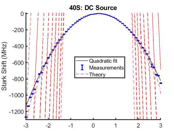
5

TABLE II. Experimentally obtained calibration constants.       TABLE III. Experimentally obtained αe (0), percentage error
The uncertainty is the standard deviation of the calibration   from calculated α(0), and experimentally obtained plate sep-
constant obtained from the 6 sets of data.                     arations. The uncertainty is the standard deviation from 6
                    Calibration Factors                        sets of data..
                                       √                         Rydberg state      αe (0)    ∆% Plate separation (mm)
             Rydberg state CCal (V/ Hz)
              28S1/2 Cell 1 (339 ± 2.7) · 10−6                  28S1/2 Cell 1 83.95 ± 1.4 0.29           2.20 ± 0.019
              40S1/2 Cell 1 (96.7 ± 0.2) · 10−6                 40S1/2 Cell 1 1032.43 ± 4.4 2.4          2.21 ± 0.005
              47S1/2 Cell 1 (53.8 ± 0.3) · 10−6                 47S1/2 Cell 1 3328.59 ± 33.2 1.6         2.16 ± 0.013

                                                               by comparing eq. (3) to eq. (4)]:
second cell (Cell 2 mentioned above) had not only tilts in
the plate, but had a twist in the plate. While not shown                            αe = 2d2 /Ccal
                                                                                               2
                                                                                                   .                    (6)
here, the measurements from the second cell showed even
more broadening and the appearance of double peaks in             Using this expression and the average plate separa-
the EIT lines.                                                 tions for the four corners (measurement with a micro-
   We extract the measured Stark shifts (corresponding         scope) given above (d = 2.194 mm for the cell), the es-
to the location of the maximum of the shifted EIT peak)        timated αe (0) for each state and each cell is given in
and plot them against the applied voltage. This was            Table III. In this table we also show the percent error
done for the three Rydberg states mentioned previously         (∆%=100*[αe (0) − α(0)]/α(0)], where α(0) is given in
(28S, 40S, and 47S), shown by Fig. 6. The error bars           Table I). Better control of the plate separation would al-
in these plots correspond to the standard deviation from       low for more accurate determination of αe (0).
six sets of data. In this data, we can also identify that
the Stark shift is not zero for zero applied voltage. This
offset is possibly due to excess charge in both vapor cells.   V.   ENERGY LEVEL CROSSINGS
Grounding the two plates did not remove this excess
charge. The voltage offset comes from various sources,            The measured data in Fig. 6 were corrected for the
including (1) impurities in the metal causing a build up       voltage offset and compared to theoretical calculations
of charge which cannot be removed and (2) ionization           for the Stark shift. The theoretical Stark maps were
caused by the 480 nm coupling laser. It is also possible       obtain by using the Alkali Rydberg Calculator Python
that this is a result of a galvanic potential. Whatever the    package43 . These comparisons are shown in Fig. 6, where
case may be this offset can be accounted for.                  the theoretical model accounts for ELCs from nearby
   In order to determine the offset, we fit to the equation    Rydberg states. We show plots for the Stark shift as
                                                               a function of applied V . In the theoretical curves, the
                        1          2                           E field was determined using E = V d (where we use
                  ∆=    2 (V − Vo )
                       Ccal
                                     .                  (5)
                                                               d = 2.19 mm). We can see good consensus between the
                                                               experimental data and theoretical model. In particular,
where Vo is the offset voltage caused by the excess charge.    on closer inspection, the locations of the ELCs can be
We found the voltage offset is 235 ± 6 mV for this             seen in the measured data. This is further illustrated in
cell. These fits were within a 95 % confidence interval.       Fig.7, where we show an expanded view of the ELC for
Through the fit, we are also able to find the calibration      the 28S1/2 state spectra, shown in Fig. 6 (a). In this
factor for each cell as measured using the three Rydberg       figure, the level crossings are easily seen as a splitting in
states, given in Table. II. Fig. 6 shows these fits for the    the spectra around -11.2 V and -12.5 V. On this note,
three states. In determining the calibration factor Ccal       the Stark shifts corresponding to the ELCs can be used
care must be taken to ensure the ELCs do not influence         to find the calibration factor as well.
its value. The effect of the ELCs are discussed in the            After obtaining a consensus on the calibration constant
next two sections.                                             through multiple measurements, we can utilize the cells
   In addition to this, Ccal can be used to either esti-       for measuring dc voltages. However, the ELCs can limit
mate the polarizability α(0) or to determine the plate         the maximum voltage that can be accurately measured
separation. In the first case, the calibration factor found    since they cause deviations from a perfect quadratic de-
through the fit of the Rydberg atom Stark shift mea-           pendence of the frequency on the applied voltage. For a
surements and the independently measured plate sepa-           given state, it would be best to avoid voltage levels where
rations can be used to quantify the polarizability αe . In     the first ELCs appear. For example, this occurs at ap-
the second case, the calibration factor and theoretically      proximately 12 V, 1.5 V, and 0.6 V, for 28S1/2 , 40S1/2 ,
calculated polarizability can be used to find the plate        and 47S1/2 respectively. The quadratic behavior depicted
separation. In the first case, if the plate separation can     in eqs. (1) and (3) fails near the ELCs. As such, using the
be independently determined, then Ccal can be used to          eq. (4) and measured Stark shifts will need to be limited
experimentally determine αe by the following [obtained         to voltages well below the first ELC. So for large voltage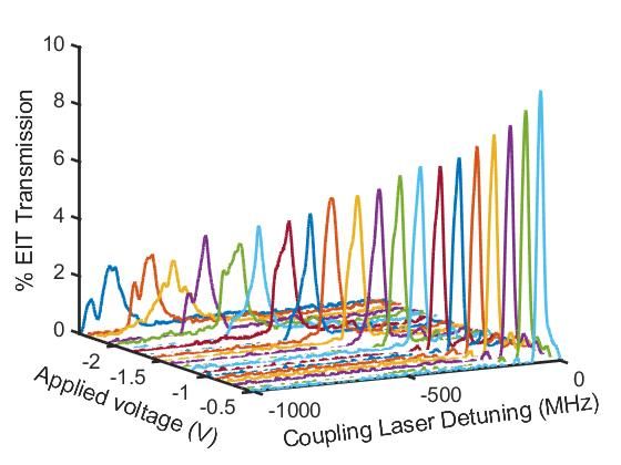
6

      FIG. 5. EIT signals (for scanning the coupling laser) showing Stark shifts for various applied voltages for 40S1/2 .

measurements Rydberg states with low n should be used,            that the EIT line shape begins to change. Such effects
while for small voltages Rydberg states with high n are           are due to E-field inhomogeneity in the region near the
more suitable (due to the higher sensitivity to weak fields       edge where the fringing fields are present (in this case the
for high n). Alternatively, choosing the electrode plate          beams are approaching two sharp corners of the plates).
separation, or manufacturing a variety of plate separa-           The angle of the cell relative to the incident angle of the
tions in a cell (with care and attention to fringing fields       beam will play a large role in the broadening as well.
and geometrical accuracy) allows a given voltage to pro-          With that said, such effects can be accounted for in a
duce a field appropriate for accurate measurement by a            calibration. In such calibrations, one needs to be careful
particular Rydberg state n.                                       when double peaks appear. These double peaks can be
                                                                  the result of imperfections in the plate manufacturing.

                                                                     In the case of the ELCs, we analyze their effect on the
VI.   SUBTLETIES TO CALIBRATION
                                                                  fit of eq. (5). Ideally, the quadratic Stark effect should fit
                                                                  the data well, but the ELCs introduce higher order terms.
   In practice, a calibration must account for or cor-            This can introduce errors in the fit of the data used to
rect three non-idealities: non-uniformity (spatial regions        find the calibration constant Ccal . Therefore, we ana-
where the electric field between electrodes departs from          lyzed how the calibration factors and fits change if we in-
the relationship E=V/d, from fringing fields or imper-            cluded different voltage ranges (max voltage-min voltage,
fections in plate manufacturing), spectroscopic features          centered at 0 V) during the fitting process. Fig. 9 shows
due to ELC interference (or “line pulling”), and a voltage        the difference between the data and the fit [i.e., eq. (5)]
offset caused by stray charge accumulation, galvanic po-          for different voltage ranges given by the separate traces.
tentials, or other stray electric field sources. We discuss       Fig. 9(a) shows the difference (i.e., residuals), Fig. 9(b)
each of these below.                                              shows the studentized residuals (|residual|/standard de-
   The fringing fields at the edge of the plate can cause a       viation), and Fig. 9(c) shows the calibration factors ob-
broadening of the EIT line. Fig. 8 shows the EIT signal           tained from the fits for different voltage ranges. Here,
for an applied voltage of 0.3 V as the optical beams are          we plot the percent difference between the data and the
moved from the center of the plates (x=7.6 mm) to the             fit for cases where we include different voltage ranges for
edge of plates (x=0 mm). Recall the optical beams are             the different fit traces for the 28S1/2 state. Note that
propagating along the the long dimension of the plates.           the large deviations for < 2 V in Fig. 9(b) are a result of
In this figure, we see the EIT signal becomes broader             the smaller error for the smaller voltages applied. This
as the beams approach the edge of the plate and we see            is due in part to the increase in width of the EIT peak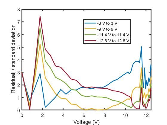
7
(a)
(b)
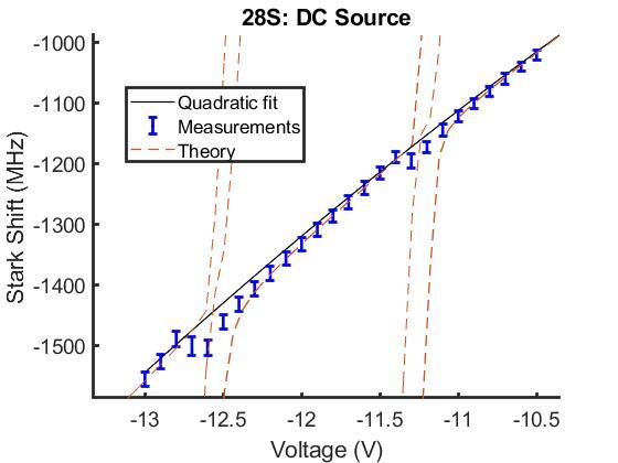
FIG. 7. Expanded view of the ELC’s for the 28S1/2 state.
We can observe the measurement (blue error bars) deviations
from the quadratic nature (solid black line) of the dc Stark
effect at these locations. Also shown is the theory (red dashed
line) that accounts for the ELC’s and matched the data much
better.
(c)
FIG. 6. (a)-(c) correspond to the measured Stark shift for 28S,
40S, and 47S Rydberg states with a dc source (blue errorbars).
Also shown are the curve fits using the calibration factor found
by eq. (5). The dashed-red lines are from theory and when
these lines become vertical indicate the position of the ELCs.
as a voltage is increased. For smaller voltages, the stan-
dard deviation was less than 1 mV for the peaks with
smaller widths, leading to increased fluctuations. It can
be seen that the fit with the least deviation is for the FIG. 8. EIT signal as the optical beams approach the edge of
case where we use voltages from -9 V to 9 V, correspond- the plate. The plate has a width of 18 mm, the edge of the
ing to a range of 18 V. In any other case, the fit breaks plate is define at x=0 mm and the center of the plate is at
from the data very quickly. The fits shown in Fig. 6 and 9 mm from the edge.
the calibration factor Ccal given above were obtained by
optimizing the voltage range in this manner.
Also shown in Fig. 9(b) are the effects of the ELCs which result in a higher order dependence and do not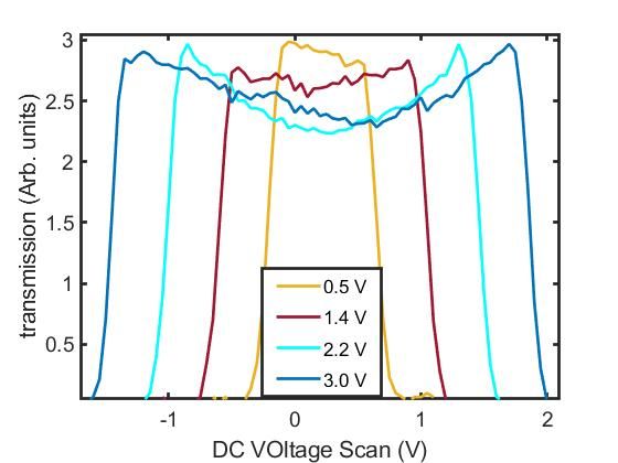
8

        (a)                                                        specific operating conditions. By tuning the plates, we
                                                                   change the necessary voltage to produce a given electric
                                                                   field.

                                                                      In the case of the voltage offset, we found that a po-
                                                                   tential cause is the combination of fringing fields and the
                                                                   charge density present on the plates. As our parallel
                                                                   plates are not infinite, there are contributions which arise
                                                                   from edge effects. These effects have a particularly strong
                                                                   response if the cell is translated horizontally, shown by
                                                                   Fig. 10. In this case, we mean perpendicular to the opti-
                                                                   cal beams and parallel to the plates. As the cell position
        (b)                                                        is moved so that the optical beams are at the edge of
                                                                   the plates (0 mm trace in Fig. 10), we observe that the
                                                                   voltage offset decreases.

        (c)

                                                                   FIG. 10. Stark shift measurements for different horizontal
                                                                   beam positions parallel to the plates. The edge of the cell is
                                                                   at 0 mm and 7.62 mm is near the center of the cell.

FIG. 9. (a) Difference (residuals) between the experimental
data and the fit in Fig. 6. (b) Studentized residuals from (a).       While the positioning of the cell changes the voltage
Each trace is for a fit incorporating data from the negative       offset, it does not change the shape of the curve. With
voltage out to the positive voltage, as labeled. (c) The cali-     the exception of the beam position at the very edge of the
bration factor obtained from fits using different voltage ranges   cell, the calibration factor changed by less than 2 % for
plotted against half the voltage range. This data is for the       the other measurements. So long as the the calibration
28S Rydberg state.                                                 curve is acquired and the voltage offset is accounted for,
                                                                   this method has potential as a standard of measurement.
                                                                   However, at the edge of the cell, there is an increased
simply follow the quadratic Stark effect. This is further          uncertainty in measurement.
demonstrated in Fig. 9(c), where we see how the calibra-
tion factor changes for the different voltage ranges used             Finally, non-uniform plate separation can be an issue
in the fit. As expected, we see under fitting if not enough        for these Rydberg atom sensors. One remedy is to use a
data is used (magenta region), a nearly flat line with-in          microfabricated cell58 to insure plate uniformity, where
error for the region of good fit (green region), and then a        microfabrication of a vapor cell allows for better control
skew of the slope as the voltage range is increased into the       of the plate or electrode separation as described in Ref.56 .
region of the ELCs (red region). To overcome the effects           The use of similar vapor cells with internal electrodes are
of the ELCs at higher voltages, we can use a more precise          currently being investigated for voltage measurements
model to account for their effects, shown by Fig. 6. The           and other applications39 . However, in this type of cell,
other option is to tune to different Rydberg states to tune        care needs to be taken to ensure that any coating placed
the sensitivity or adjust the plate separation. The latter         on the electrodes does not cause shielding of the applied
requires the use of several different cells manufactured for       voltage and in turn the E-field seen by the atoms38 .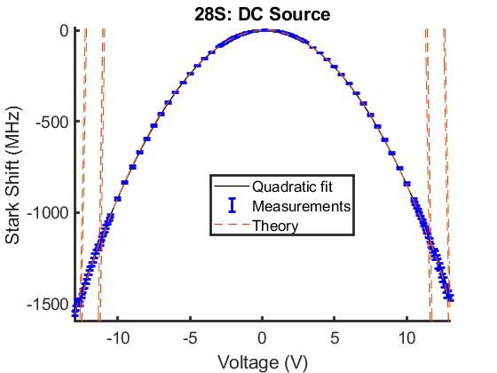
9

VII.   AC VOLTAGE MEASUREMENTS

   In addition to dc measurements, this same system can
be used to determine 60 Hz ac field strengths. However,
60 Hz ac voltage measurement require different read-out
methods. The ac Stark effect would result in a linear
shift to the EIT peak, but we instead rely on the slowly
changing dc Stark effect in the adiabatic limit where the
frequency is slow enough such that the atoms can re-
spond. This limits the measurements to the range of
frequencies from dc to 1 MHz; we work with 60 Hz. In
this application, we observed that the EIT peak shifts
from the 0-voltage location to the peak-voltage location,
as expected. Since, the calculated polarizability for the
dc and ac fields are nearly identical, this peak voltage lo-
cation also corresponds to the equivalent dc voltage. So
by tracking the maximum EIT peak shift, we can make a
calibration curve that matches the curve for a dc source,
shown in Fig. 11.
   For detecting 60 Hz ac volatge, one might consider
sweeping a laser fast enough to track the EIT as the 60 Hz
source caused it to oscillate from peak-voltage location to
zero-voltage location. Unfortunately, such a method re-
quires the laser to scan over a GHz in frequency at a scan
frequency much larger than the source bandwidth. Such
a scan speed for CW systems results in mode instability
and loss in lasing. Here, we demonstrate two alterna-
tive methods for determining the peak to peak voltage of
the source from the motion of the EIT peak. The first
method (Stark shift tracking) relies on similar scans to
the ones in the dc voltage measurements. The coupling
laser is scanned over a frequency range while 20 traces
of the transmission spectrum are gathered. During this
time, the EIT peak is oscillating between the 0-voltage
location and the peak-voltage location. We take the 20
traces and find the variance at each detuning, shown in
Fig. 12. Using this data, we find the maximum shift at
the location where the data drops off below a threshold
value that lies above the noise. The extracted drop-off lo-
cations are plotted in Fig. 11 for the three different states
also used for the dc measurements. Also plotted are the         FIG. 11. Figure shows the Stark shift plotted against the
dc data to show the agreement in the calibration between        peak voltage of an 60 Hz ac source for the three states 28S
the dc data and the ac data taken with this method.             (a), 40S (b), and 47S (c). Also included for comparison are
   Unfortunately, there is more noise in the ac data than       the dc experimental data from Figs. 6(a)-(c)
in the dc data. This noise is due to the accuracy of deter-
mining the drop-off location, which becomes increasingly
more difficult for higher ac voltages. At higher voltages,      pendent shift in the drop-off location. However, this is
the drop-off almost smooths to the level of the noise. The      not apparent here within the bounds of error.
dc data did have a similar issue for the higher voltages,          The second method (dc biased ac sensing) relies on the
but because of the averaging of the peak at one location,       use of a dc calibrated source. As discussed previously,
it was mitigated. With an ac source, this option is not         if we have an ac source on the plates, the EIT peak
available and for the interest of time and as a demon-          will oscillate between the zero-voltage location and the
stration, we only used 20 traces. However, by collecting        peak-voltage location. We can observe this shifting if we
more traces, we should be able to bring the noise down.         scan the coupling laser. However, if we lock the coupling
Further sources of error or deviation from the calibra-         laser to the zero-voltage location, we will instead observe
tion could also be present from the imperfections in the        transmission only when the ac voltage passes through the
plates of the cell. The EIT peak widths broadens with           zero-voltage location, as shown by the computer gener-
voltage and this could potentially result in a voltage de-      ated plot in Fig. 13 (a). This produces a transmission
10

                                                                  We track the height of the transmission peaks in Fig. 13.
                                                                  As we scan the dc voltage source from -2 V to 2 V, we can
                                                                  see the transmission appear and then vanish, as shown
                                                                  in Fig. 14 (a). The voltage difference in the two drop-off
                                                                  locations in the dc voltage scan defines the peak to peak
                                                                  voltage of the applied ac voltage. Fig. 14 (a) shows the
                                                                  traces of dc voltage scan for several different ac voltages
                                                                  and Fig. 14 (b) shows the extracted peak to peak voltages
                                                                  plotted against the applied voltage.
                                                                     DC biased ac sensing has certain advantages when
                                                                  compared to Stark shift tracking. In the case of Stark
                                                                  shift tracking, we must average for a long time to im-
                                                                  prove the statistics enough to measure larger voltages.
                                                                  However, for dc biased ac sensing, we do not have this
                                                                  same limitation since the measurement occurs at the
FIG. 12. Sample of variance of 20 traces plotted against the      zero-voltage location with maximum EIT peak height.
coupling laser detuning for a 1.2 V AC source for the 40S
                                                                  Unfortunately, the maximum ac voltage we can sense is
state. As the EIT peak shifts around, the variance increases
in the regions where it has passed.                               limited by the range of our calibrated dc source. While
                                                                  this voltage is higher than measurements with the Stark
                                                                  shift tracking method, it is still limited. Furthermore,
    1 V peak to peak + 0 V DC offset
                                                                  this method requires a laser lock that is stable to less
                                                                  than 1 MHz for the probe and coupling lasers.
     (a)

    1 V peak to peak + 0.25 V DC offset                           VIII.   CONCLUSION AND DISCUSSION

                                                                      In this manuscript, we have demonstrated a means to
     (b)                                                          an alternative voltage standard based on the inherent
                                                                  and known dipole strengths of Rydberg atoms and have
    1 V peak to peak + 0.5 V DC offset                            filled the SWAP-C gap between Zener diode and Joseph-
                                                                  son junction based standards in doing so. By measuring
                                                                  the dc Stark shift for various voltages at different states,
     (c)                                                          we generate a calibration standard which can be utilized
                                                                  as an alternative to two established voltage measurement
    1 V peak to peak + 0.75 V DC offset                           technologies. In addition to this, we discuss how the cal-
                                                                  ibration factor Ccal can be used in two ways. First, if
                                                                  the plate separation is known, the calibration factor can
     (d)
                                                                  be used to determine the polarizaibility for the Rydberg
                                                                  states. Secondly, we discuss how calibration factors can
                                                                  be used to find the plate separation to within 10s of mi-
FIG. 13. Sample showing expected EIT transmission (blue)
                                                                  crons. We also demonstrate two methods to measure
in the presence of a 60 Hz ac field (red) plotted against the     60 Hz ac sources with little to no modification to the
phase of the applied ac field. The plots correspond to offset     apparatus.
voltages of (a) 0 V, (b) 0.25 V, (c) 0.50 V, and (d) 0.75 V, as       In the case of dc sources, we were able to find Stark
labeled.                                                          shifts (∆) within an average error under ±5 MHz over
                                                                  6 sets of data. Even though there was broadening of
                                                                  the EIT peak and contributions from inhomogeneities at
peak that we can monitor that is dependant on the ac              larger voltages, the uncertainty in the voltage did not
voltage source. Now, if we apply a calibrated dc volt-            change since the sensitivity increases with larger voltages.
age along with the ac voltage the transmission peak will          The fractional uncertainty in the voltage is given by
shift since the ac voltage at which the voltage sum crosses                       2               2                2                2
zero is no longer when the ac voltage passes zero, shown                      δV                δd                 δα                 δ∆
in Figs. 13 (b) and (c). However, if the dc voltage is                                  =                 +                  +                  .   (7)
                                                                               V                d                 2·α                2·∆
increased to a value higher than the peak voltage, the
transmission will begin to vanish, as shown in Fig. 13            The error in the Stark shift measurement translated to
(d).                                                              a fractional uncertainty in the voltage is on the order of
   In this method, we apply a calibrated dc voltage as an         .01 V/V on average over the voltage range of the 47S Ry-
offset to an ac voltage source that we wish to determine.         dberg state. The fractional uncertainty is constant due
11
(a) (b)
FIG. 14. (a) Sample of traces for different ac voltages where the peak transmission is plotted against the calibrated dc voltage.
(b) The width of the traces in (a) that correspond to the peak to peak voltage, plotted against the applied peak to peak voltage
(V). This data is for the 47 S state. (black) is the one-to-one line as a guide and the (blue) is the extracted ac voltage.
to the broadening of the EIT peak at higher applied volt- We analyzed various sources of uncertainty that arose
ages, as discussed previously. The 20 sets averaged to find from non-uniform electric fields, ELCs, and plate imper-
a given Stark shift have scan times of 25 ms. This corre- fections. The combination of these effects initially point
sponds to a sensitivity in the voltage measurement on the to the infeasibility of the Rydberg atom as a voltage stan-
order of 0.007 V/V Hz −1/2 using the 47S state. While dard, but through careful consideration and calibration,
this level of sensitivity seems limited, different Rydberg these problems can be accounted for. We discussed the
states can be used for increased sensitivity. By simply broadening of the EIT lines due to non-uniform fields,
choosing to work at the 28S state, the uncertainty in the EIT line perturbations from fringing fields at the edge
measurement decreases to 0.003 V/V. This is due to the of the plates, and the effects of the ELCs on the EIT
stronger EIT peak at the 28S Rydberg state. The sen- spectra. These considerations are key to developing a
sitivities of these voltage measurements are ultimately portable Rydberg standard and will affect the sensitiv-
limited by several aspects. One is that the polarizability ity, range, and reliability for future atom based voltage
can only be calculated to an uncertainty of 1%. However, sensors. In conclusion, this study on the dc and 60 Hz ac
certain experimental techniques can determine the polar- fields will provide insight for future advancements for the
izabilities of atoms to a much better accuracy57 . Another realization of a self-calibrating, deployable voltage stan-
key factor is in the time domain. The laser sweep must dard. Future work will include developing vapor cells
be able to span several GHz for these measurements and with more precise plate separation, including microfabri-
thus sets a limit on how fast data can be collected. Fi- cated cells.
nally, the ultimate determination of how well the Stark We emphasize that a future device could be made
shift can be measured depends on the linewidth and am- where instead of being calibrated, the polarizability and
plitude of the EIT line. This is currently 15 MHz in plate spacing could be accurately measured and then the
our system. Similar Rydberg techniques have demon- device would be based on fundamental standards. Other
strated linewidths down to 2 MHz7 . This is nearly an questions to be answered in future work is how the reso-
order of magnitude improvement that can be achieved. lution, stability and fractional uncertainties compare to
Furthermore, new three-photon configurations may offer Zener diodes systems.
linewidths under 100 kHz which could offer over an order
of magnitude improvement53 . In addition to this, for in-
creased voltages, we begin to see effects from energy level IX. ACKNOWLEDGEMENT
crossings and plate inhomogeneities. The prior can be ad-
dressed by adjustments to the quadratic fit and the latter The authors thank Dr. Yuan-Yu Jau with Sandia Na-
by the manufacturing of a more uniform plate geometry, tional Labs, Albuquerque, NM 87123, USA for his useful,
as our current plates have a dimple (and discontinuities) insightful technology discussions, and for suppling one of
in the very center where the leads are mounted. These the vapor cells used in our experiments.
improvements are complementary and would increase the
range of voltages accessible and improve our sensitivity
to better than 10−5 V /V Hz −1/2 . X. DATA AVAILABILITY STATEMENT
Data is available upon request.12 1 T.F. Gallagher, Rydberg Atoms. Cambridge Univer. 29 P.D. Dresselhaus, S.P. Benz, C.J. Burroughs, N.F. Bergen, Y. Press:Cambridge, 1994. Chong, ”Design of SNS Josephson arrays for high voltage applica- 2 A.K. Mohapatra, T.R. Jackson, and C.S. Adams, Phys. Rev. tion”, IEEE Transactions on Applied Superconductivity, 17(2), Lett., 98, 113003, 2007. 173-176, 2007. 3 J.A. Gordon, C.L. Holloway, S. Jefferts, T. Heavner, “Quantum- 30 T. Yamada, H. Yamamori, H. Sasaki, A. Shoji, Japanese Journal Based SI Traceable Electric-Field Probe,” Proc of 2010 IEEE In- of Applied Physics, 48(7R), 076510, 2009. ternational Symposium on Electromagnetic Compatibility, July 31 O. Rest, D. Winzen, S. Bauer, R. Berendes, J. Meisner, T. 25-30, 321-324, July 2010. Thuemmler, S. Wuestling, C. Weinheimer, ”A novel ppm-precise 4 J.A. Sedlacek, A. Schwettmann, H. Kubler, R. Low, T. Pfau and absolute calibration method for precision high-voltage dividers”, J.P. Shaffer, Nature Phys., 8, 819, 2012. Metrologia, 56, 045007, 2019. 5 C.L. Holloway, J.A. Gordon, A. Schwarzkopf, D.A. Anderson, 32 Witt, T.J., Reymann, D., and Avrons, D., IEEE. Trans. on In- S.A. Miller, N. Thaicharoen, and G. Raithel, IEEE Trans. on strumentation and Measurement, 44(2), 226-229, 1995. Antenna and Propag., 62(12), 6169-6182, 2014. 33 Witt, T.J., Proc. IEE Sci. Meas. Technol., 149(6), 305-312, 6 C.L. Holloway, M.T. Simons, J.A. Gordon, P.F. Wilson, C.M. 2002. Cooke, D.A. Anderson, and G. Raithel, IEEE Trans. on Electro- 34 T. Middelmann, S. Falke, C. Lisdat, U. Sterr, ”High accuracy cor- magnetic Compat., 59(2), 717-728, 2017. rection of blackbody radiation shift in an optical lattice clock”,T 7 Kumar, S., Fan, H., Kübler, H. et al.,Sci Rep, 7, 42981 (2017). Middelmann, S Falke, C Lisdat, U Sterr, ”High accuracy cor- 8 Tanasittikosol, M., Pritchard, J.D., Maxwell, D., Gauguet, A., rection of blackbody radiation shift in an optical lattice clock”, Weatherill, K.J., Potvliege, R.M., and Adams, C.S., J. Phys B, Physical Review Letters, 109, 263004, 2012. 44, 184020, 2011. 35 J.A. Sherman, N.D. Lemke, N. Hinkley, M. Pizzocaro, R.W. 9 C.L. Holloway, J.A. Gordon, A. Schwarzkopf, D.A. Anderson, Fox, A.D. Ludlow, C.W. Oates, ”High-accuracy measurement of S.A. Miller, N. Thaicharoen, and G. Raithel, Applied Phys. Lett., atomic polarizability in an optical lattice clock”, Physical Review 104, 244102-1-5, 2014. Letters, 108, 153002, 2012. 10 J. A. Gordon, C. L. Holloway, A. Schwarzkop, D. A. Anderson, 36 J.M. Amini, H. Gould, ”High precision measurement of the static S. Miller, N. Thaicharoen, G. Raithel, Applied Physics Letters, dipole polarizability of cesium”, PRL, 91(15), 153001, 2003. 105, 024104, 2014. 37 M.D. Gregoire, I. Hromada, W.F. Holmgren, R. Trubko, A.D. 11 Gordon, J.A., et al., AIP Advances, 9, 045030, 2019. Cronin, ”Measurements of the ground-state polarizabilities of Cs, 12 J.A. Sedlacek, A. Schwettmann, H. Kubler, and J.P. Shaffer, Rb, and K using atom interferometry”, PRA 92, 052513, 2015. Phys. Rev. Lett., 111, 063001, 2013. 38 Daschner, R., Ritter, R., Kübler, H. Frühauf, N., Kurz, E., Löw, 13 M.T. Simons, A.H. Haddab, J.A. Gordon, and C.L. Holloway, R., and Pfau, T., Optics Letters, 37(12), 2271-2273, 2012. IEEE Access, 7, 164975-164985, 2019. 39 Daschner, R., Kübler, H., Löw, R., Baur, H. Frühauf, N., and 14 M.T. Simons, A.H. Haddab, J.A. Gordon, and C.L. Holloway, Pfau, T., Applied Phys. Letters, 105, 041107, 2014. Applied Physics Letters, 114, 114101 2019. 40 M.G. Bason, M. Tanasittlosol, A. Sargsyan, A.K. Mohapatra, 15 Jing, M., Hu, Y., Ma, J., Zhang, H., Zhang, L., Xiao, L., and D. Sarkisyan, R.M. Potvliege, and C.S. Adams, N. Journal of Jia, S. Nat. Phys., 16, 911–915, 2020. Physics, 12, 065015, 2010. 16 C.L. Holloway, M.T. Simons, M.D. Kautz, A.H. Haddab, J.A. 41 Osterwalder A., and Merkt, F., Phys Review Letters, 82(9), 1831- Gordon, T.P. Crowley, Applied Phys. Letters, 113, 094101, 2018. 1834, 1999. 17 Meyer, D.H., Kunz, P.D., and Cox, K.C., Physical Review Ap- 42 H. Friedrich. Theoretical Atomic Physics. 4th Edition, Springer, plied, 15, 014053, 2021. 2017. 18 Robinson, A., Simons, M.T., and C.L. Holloway, Applied Phys. 43 Elizabeth J. Robertson and Nikola Šibalić and Robert M. Lett., 118(11), 114001, doi.org/10.1063/5.0045601, 2021. Potvliege and Matthew P. A. Jones, ARC 3.0: An expanded 19 Z. Song,H. Liu, X. Liu, W. Zhang, H. Zou, J. Zhang, and J. Qu, Python toolbox for atomic physics calculations, arXiv eprint ‘Optics Express 27(6), 2019. 2007.12016 (2020). 20 D.H. Meyer, K.C. Cox, F.K. Fatemi, and P.D. Kunz, Appl. Phys. 44 Jianing Han, Yasir Jamil, D. V. L. Norum, Paul J. Tanner, and Lett., 12, 211108, 2018. T. F. Gallagher, Phys. Rev. A, 74, 054502 (2006) 21 C.L. Holloway, M.T. Simons, A.H. Haddab, J.A. Gordon, D. 45 V. A. Yerokhin, S. Y. Buhmann, S. Fritzsche, and A. Surzhykov, Novotny, IEEE Antenna and Wireless Propag. Lett. 18(9), 1853- Phys. Rev. A, 94, 032503 2016. 1857, 2019. 46 M. S. O’Sullivan and B. P. Stoicheff, Phys. Rev. A 31, 2718 1985. 22 K.C. Cox, D.H. Meyer, F.K. Fatemi, and P.D. Kunz, “Quantum- 47 M. S. O’Sullivan and B. P. Stoicheff, Phys. Rev. A 33, 1640 1986. Limited Atomic Receiver in the Electrically Small Regime”, 48 D. Das and V. Nataranjan, “High-precision measurement of hy- Phys. Rev. Lett. 121, 110502, 2018. perfine structure in the D lines of alkalai atoms”, J Phys B, 41, 23 C.L. Holloway, M.T. Simons, A.H. Haddab, J.A. Gordon, and S. 035001, 2008. Voran, “A Multi-Band Rydberg-Atom Based Receiver: AM/FM 49 D. A. Steck, “Rubidium 85 D line data”, revision 2.1.6 Sep. 20, Stereo Reception”, accepted to appear in IEEE Antenna and 2013 [Online]. Available: http://steck.us/alkalidata. Propogation Magazine, 2021. 50 M.T. Simons, A.H. Haddab, J.A. Gordon, and C.L. Holloway, 24 D.A. Anderson, R.E. Sapiro, and G. Raithel, “An atomic receiver “Applications with a Rydberg Atom-based Radio Frequency An- for AM and FM radio communication”, arXiv:1808.08589v1, tenna/Receiver,” Procc in EMC EUrope 2019, Barcelona, Spain, Aug. 26, 2018. Sept. 2019. 25 S. Ottoa, M.K. Hunter, N. Kjærgaard, and A.B. Debb, “Data 51 M. T. Simons, M. Kautz, J. A. Gordon, and C. L. Holloway, “Un- capacity scaling of a distributed Rydberg atomic receiver array”, certainties in Rydberg atom-based RF E-field measurements,” in Journal of Applied Physics, 129, 154503, 2021. Proc. EMC Europe, Amsterdam, The Netherlands, Aug. 2018, 26 Holloway, C.L., Simons, M.T., Haddab, A.H., Williams, C.J., pp. 376-380. and Holloway, M.W., AIP Advanced, 9(6), 065110, 2019. 52 H. Fan, S. Kumar, J. Sheng, J.P. Shaffer, C.L. Holloway and J.A. 27 Rüfenacht, A., Flowers-Jacobs, N.E., and Benz, S.P., Metrologia Gordon, Physical Review Applied, 4, 044015, November, 2015. 55, S152-S173, 2018. 53 J. P. Shaffer and H. Kübler, “A read-out enhancement for mi- 28 Y. Tang, V.N. Ojha, S. Schlamminger, A. Ruefenacht, C.J. Bur- crowave electric field sensing with Rydberg atoms,” Proc of SPIE roughs, P.D. Dresselhaus, S.P. Benz, ”A 10 V programmable Photonics Europe, July, 39-49, July 2018. Josephson voltage standard and its applications for voltage 54 P.R. Berman and V.S. Malinovsky, Priciples of Laser Spec- metrology”, Metrologia, 49, 635-43, 2012. troscopy and Quantum Optics. Princeton Univerity Press, 2011.
13

55 M.G.  Bason, Coherent atom-light interactions in multi-level sys-      of polarizabilities of cesium nS Rydberg states in an ultra-cold
   tems. PhD. Thesis, Department of Physics, Durham University,           atomic ensemble, New Journal of Physics,22(9), 093032, 2020.
   chapter 7, Oct 20, 2009.                                            58 J. Kitching, E.A. Donley, S. Knappe, M. Hummon, A.T. Dellis,
56 L.A. Liew, S. Knappe, J. Moreland, H. Robinson, L. Hollberg,           J. Sherman, K. Srinivasan, V. A. Aksyuk, Q. Li2, D. Westly, B.
   and J. Kitching, Applied Phys. Letters, 84(14), 2694-2996, 2004.       Roxworthy A.Lal, , Journal of Physics: Conference Series, 723,
57 Jingxu Bai and Suying Bai and Xiaoxuan Han and Yuechun                 012056, 2016.
   Jiao and Jianming Zhao and Suotang Jia, Precise measurements
You can also read