Full-depth desalination of warm sea ice - Archive ouverte HAL
←
→
Page content transcription
If your browser does not render page correctly, please read the page content below
Full-depth desalination of warm sea ice
    Fernanda Jardon, Frédéric Vivier, Martin Vancoppenolle, Antonio Lourenço,
                         Pascale Bouruet-Aubertot, yannis Cuypers

     To cite this version:
    Fernanda Jardon, Frédéric Vivier, Martin Vancoppenolle, Antonio Lourenço, Pascale Bouruet-
    Aubertot, et al.. Full-depth desalination of warm sea ice. Journal of Geophysical Research. Oceans,
    Wiley-Blackwell, 2013, 118 (1), pp.435-447. �10.1029/2012JC007962�. �hal-01139061�

                                 HAL Id: hal-01139061
                https://hal.archives-ouvertes.fr/hal-01139061
                                     Submitted on 4 Jan 2022

    HAL is a multi-disciplinary open access            L’archive ouverte pluridisciplinaire HAL, est
archive for the deposit and dissemination of sci- destinée au dépôt et à la diffusion de documents
entific research documents, whether they are pub- scientifiques de niveau recherche, publiés ou non,
lished or not. The documents may come from émanant des établissements d’enseignement et de
teaching and research institutions in France or recherche français ou étrangers, des laboratoires
abroad, or from public or private research centers. publics ou privés.
                                              Copyright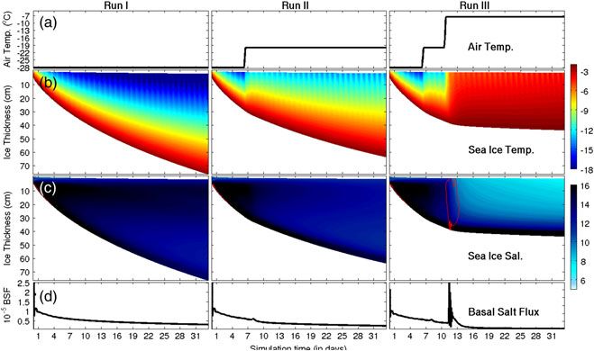
JOURNAL OF GEOPHYSICAL RESEARCH: OCEANS, VOL. 118, 435–447, doi:10.1029/2012JC007962, 2013

Full‐depth desalination of warm sea ice
F. P. Jardon,1 F. Vivier,1 M. Vancoppenolle,2,3 A. Lourenço,1 P. Bouruet‐Aubertot,1 and
Y. Cuypers1
Received 7 February 2012; revised 27 September 2012; accepted 21 November 2012; published 31 January 2013.

[1] The large‐scale Arctic sea‐ice retreat induces a gradual replacement of thick, multi‐
year sea ice by thinner first‐year ice. The latter has distinctive physical properties and is in
particular substantially saltier. It is generally thought that while salt rejection occurs
primarily during ice formation in winter, most of the remaining brine is flushed out of the
ice by the percolating surface melt water in summer. Here, it is argued that a substantial
part of this residual desalination of first‐year sea ice can occur well before summer melt,
due to brine convection over the full thickness of the ice, once the ice temperature is higher
than a threshold that depends on bulk salinity and thickness. This critical temperature is
substantially higher than the permeability threshold. The argument stems from a theoretical
analysis of the porous Rayleigh number depicting the propensity for convection in the
mushy‐layer theory. It is supported by simulations performed with a state‐of‐the‐art 1‐D
sea‐ice model. The study was initially motivated by observations collected in March 2007
in Storfjorden, Svalbard. Those are indirect, however, and are thus presented here as a
possible example. Two sporadic anomalies of seawater salinity were recorded close to the
base of 40cm thick ice in temperature conditions that are incompatible with ice formation.
Analyses and simulations forced with observed atmospheric conditions suggest that the
second peak is caused by flushing of meltwater, while the first and most intense peak is
likely associated with an episode of brine convection over the full depth of the ice, yielding
significant desalination.
Citation: Jardon, F. P., F. Vivier, M. Vancoppenolle, A. Lourenço, P. Bouruet-Aubertot, and Y. Cuypers (2013),
Full-depth desalination of warm sea ice, J. Geophys. Res. Oceans, 118, 435–447, doi: 10.1029/2012JC007962.

1. Introduction                                                                2007; Nghiem et al., 2007]. Recently, Maslanik et al. [2011]
                                                                               have shown that multi‐year ice now represents only 45% of
  [2] Arctic sea ice is profoundly changing. The reduction in                  the total ice extent in March, while it was 75% in the mid‐1980s.
summer sea‐ice extent evidenced by satellite data since the                      [3] The transition from a perennial to a seasonal Arctic sea
1980s [e.g., Comiso, 2002], which has accelerated in the past                  ice cover will likely feedback on climate by changing atmo-
few years with a series of record minima [Stroeve et al., 2007;                sphere‐ice‐ocean heat, salt, and freshwater fluxes [Holland
Comiso et al., 2008], occurs primarily at the expense of thick                 et al., 2006]. This shift toward thinner seasonal ice already sug-
multi‐year ice. The decline in sea‐ice extent is indeed accom-                 gests a coincident decrease in surface albedo and an increase
panied by a nearly 50% reduction of the average sea‐ice                        of solar energy absorption by the ice‐ocean system during sum-
thickness, from 3.64m in the 1980s to 1.89m in 2009, for win-                  mer melt [Perovich et al., 2002, 2007; Nghiem et al., 2007].
ter conditions [Kwok and Rothrock, 2009]. This thinning                        Multi‐year ice has lower brine content and is fresher than
mostly reflects the replacement of multi‐year ice by first‐year                  first‐year ice [e.g., Weeks and Ackley, 1986], since it has under-
ice [Haas et al., 2010]. Indeed, the average age of the sea ice                gone summer melt. Investigating the release of salt from first‐
has dramatically decreased, particularly as a result of recent                 year ice is therefore highly suited to the Arctic where the ice
regime shifts [Rigor and Wallace, 2004; Maslanik et al.,                       cover is transitioning toward a seasonal cover.
                                                                                 [4] About two thirds of the initial seawater salt content
    1
      Laboratoire d'Océanographie et du Climat (LOCEAN)‐IPSL,                  is rejected during early ice growth [e.g., Kovacs, 1996].
Université Pierre et Marie Curie, Paris, France.                               Because the ice crystalline lattice hardly tolerates impurities,
    2
      Georges Lemaître Centre for Earth and Climate Research, Earth and Life
Institute, Université catholique de Louvain, Louvain‐la‐Neuve, Belgium.        the remaining salt is nearly exclusively contained in liquid
    3
      Dept. of Atmospheric Sciences, University of Washington, Seattle,        brine inclusions. Due to brine rejection, ice loses most of
WA, USA.                                                                       its salt during its first year [e.g., Kovacs, 1996]. First‐year
    Corresponding author: F. P. Jardon, Laboratoire d'Océanographie et du      (FY) sea ice has therefore a distinct salinity profile compared
Climat ‐ Institut Pierre‐Simon Laplace, Université Pierre et Marie Curie,      with older ice, which greatly affects brine volume fraction
4 Place jussieu, Tour 45/55, 4ème étage, boîte 100, Paris, 75005, France.      (or porosity), e, and thermal properties. The ice enthalpy
(Fernanda.Jardon@locean‐ipsl.upmc.fr)                                          and thermal conductivity both decrease with increasing
©2012. American Geophysical Union. All Rights Reserved.                        salinity for a given temperature, whereas the heat capacity
2169-9275/13/2012JC007962                                                      increases [Malmgren, 1927].

                                                                           435
JARDON ET AL.: FULL‐DEPTH DESALINATION OF SEA ICE

  [5] Porosity provides a primary control on fluid transport          of the Svalbard Archipelago that hosts a latent heat polynya
within the sea ice as it determines fluid permeability. Applying      [Haarpaintner et al., 2001; Skogseth et al., 2004], which is
percolation theory to sea ice, Golden et al. [1998] suggested        prone to the formation of substantial amounts of young ice.
that ice is permeable above a critical porosity threshold of           [9] This paper is structured as follows. In section 2, we
e=5%. For a typical bulk salinity Si of 5 (throughout this           derive from theory a necessary condition for gravity drain-
paper, salinities are expressed relative to the practical salinity   age to occur over the entire thickness of the ice. Idealized
scale PSS‐78 and are thus dimensionless), ice is therefore           simulations performed with a 1‐D sea‐ice model, including
permeable when temperature Ti exceeds −5°C (based on the             a state‐of‐the‐art parameterization of salt dynamics, are
liquidus relation). This rule was referred to as the “rule of        conducted in section 3 to illustrate theoretical results. We
fives” by Golden et al. [1998].                                       then present in section 4 our observations as a possible
  [6] Among the various processes for potentially removing           example of full‐depth gravity drainage. Observations show
salt from sea ice [Untersteiner, 1968; Cox and Weeks, 1974;          two salinity peaks occurring 10h apart during a warm storm,
Eide and Martin, 1975], recent studies confirmed that only            the second of which is associated with flushing as indicated
gravity drainage and flushing contribute significantly [Notz           by model simulations. Modeling further suggests that the
and Worster, 2009; Weeks, 2010; Hunke et al., 2001]. Gravity         first and most intense peak is caused by gravity drainage
drainage results from the convection of dense, saline brine          occurring over the full depth of the ice. A concluding discus-
through permeable ice in a vertical temperature gradient, with       sion follows in section 5.
colder temperatures on the top. This temperature gradient
involves an unstable brine salinity gradient to maintain phase       2. Theory
equilibrium. Convection develops once available potential
energy (i.e., negative buoyancy) overcomes viscous dissipa-            [10] In the introduction, we claimed that gravity drainage
tion, or, quantitatively, once a porous‐medium Rayleigh num-         may not be limited to the lowermost fraction of the ice layer
ber (Ra) exceeds a critical value Rac ≈10 [Notz and Worster,         and that in some circumstances it could lead to substantial
2008]. This formulation stems from mushy‐layer theory                desalination of the ice by the downward transport of salt
[Feltham et al., 2006; Wettlaufer et al., 1997a; Worster,            throughout the full thickness of the ice.
1997], where a mushy layer is defined as a two‐phase (solid             [11] Here, we examine under which environmental condi-
ice and brine), two‐component, reactive porous medium.               tions full‐depth convection would be possible. Specifically,
Flushing refers to the washing out of brine by the percolation       we analyze the sensitivity of brine convection to the tempera-
of surface meltwater through the permeable ice matrix in             ture of the sea ice and derive a necessary condition for convec-
response to a hydrostatic head.                                      tion over the entire ice column. This condition is expressed as
  [7] Desalination of sea ice has frequently been observed to        a temperature threshold that depends on the bulk salinity and
be associated with gravity drainage during sea‐ice formation         thickness of the ice.
[e.g., Lake and Lewis, 1970; Notz and Worster, 2008] or with           [12] The propensity for brine convection (or gravity drain-
flushing during the melt season [e.g., Trodahl et al., 2000;          age) in sea ice is compactly described by mushy‐layer theory
Freitag and Eicken, 2003; Vancoppenolle et al., 2007].               [Worster, 1992; Feltham et al., 2006] using a porous‐medium
According to these studies [see also Wettlaufer et al. 1997a],       Rayleigh number, Ra [Worster, 1992; Wettlaufer et al., 1997a;
winter desalination occurs through gravity drainage, whereby         Notz and Worster, 2008]. This number reflects the ratio
convection seems to develop in a thin (~5cm) layer near the          between the energy available for convection and the energy
ice base. Convection over much wider vertical scales has been        that is dissipated during convection, owing both to the
inferred from temperature data [Pringle et al., 2007] or associ-     moving brine's viscosity and to thermal energy loss through
ated with the freezing of slush above a permeable ice layer          heat diffusion. The expression used here for Ra depends on
[Lytle and Ackley, 1996]. In contrast, observations of salinity      the vertical coordinate in the ice, as per Notz and Worster
peaks in the upper ocean associated with brine release from          [2008], and reads
sea ice are relatively sparse. Hudier et al. [1995] reported salt
rejection at the base of the ice that they associate with an                              gðhi −zÞρw βw ðSbr −Sw ÞΠðemin Þ
                                                                                   Ra ¼                                    ;      (1)
upward flushing of sea water. More recently, Widell et al.                                                κη
[2006] observed a basal salt flux from warming first‐year sea
ice in the Svalbard region in spring time, which was correlated      where g is the gravitational acceleration; hi −z is the distance
with the ocean‐ice heat flux.                                         between a given level in the sea ice z and the base of the ice
  [8] In this work, we argue that a substantial fraction of the      at depth hi; ρwβw(Sbr −Sw) is the difference between the brine
residual salt remaining in first‐year sea ice can be rejected         density at level z (with salinity Sbr) and that of the seawater
well before summer, due to gravity drainage developing               (with salinity Sw); while Π(emin) represents the effective sea‐
throughout the full thickness of the ice, once the ice is            ice permeability (in square meters), computed as a function
warmer than a temperature threshold dependent on bulk                of the minimum brine volume fraction emin between level z
salinity and thickness. This threshold is well above the             and the base of the ice. Finally, κ and η are the thermal
permeability threshold. This argument stems from theoretical         diffusivity and dynamic viscosity of the liquid brine, respec-
and modeling considerations but was initially motivated by           tively [Wettlaufer et al., 1997b; Notz and Worster, 2008].
observations. The latter are indirect; however, two sporadic         These studies assume that thermodynamical equilibrium is
positive anomalies in seawater salinity were recorded close          not maintained on the fast time scales associated with convec-
to the base of the ice in March 2007, near the end of the            tion (Dirk Notz, personal communication). The thermal diffu-
freezing season, in conditions incompatible with ice forma-          sivity of the moving liquid brine (which is one order smaller
tion. Measurements were taken in Storfjorden, a large fjord          than that of the surrounding freshwater ice) is therefore used

                                                                 436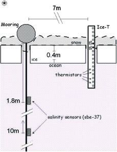
JARDON ET AL.: FULL‐DEPTH DESALINATION OF SEA ICE
in (1), rather than the bulk diffusivity of ice. Convection is salinity, Sbr, is constrained by the liquidus relationship,
triggered when the available potential energy (negative buoy- which is expressed as a third order polynomial in temperature
ancy) overcomes dissipation by a factor of ≈10 (the critical [Assur, 1958]
Rayleigh number, Rac) [Notz and Worster, 2008]. The depen-
dence of the effective permeability on the brine volume Sbr ðTi Þ ¼ −1:2−21:8Ti −0:919Ti2 −0:0178Ti3 : (2)
fraction is taken as Π(e)=10−17(103 ×e)3.1, an empirical
relationship derived by Freitag [1999]. A cubic dependence
on the porosity is predicted by the Kozeny‐Carman equation, [14] For Ti warmer than ~−6°C, the latter equation is well
which models a porous material as an assembly of capillary approximated by the linear relation Sbr(Ti)≈−Ti/μ, where
tubes [Kozeny, 1927; Carman, 1937]. Cubic dependence μ=0.054°C‰−1, which shows the direct dependence of the
is also demonstrated theoretically for a hierarchical model driving density gradient on Ti. Conversely, because the bulk
[Golden et al., 2007]. salinity of the ice Si is related to the brine salinity according
[13] To analyze the sensitivity of Ra on sea‐ice temperature to Si =Sbr ×e, one can write e(Si,Ti)≈−μSi/Ti, showing that
Ti, we explicitly introduce this variable in (1). The numerator brine volume e and permeability depend on the inverse of Ti.
of (1) is the product of the driving density gradient and perme- [15] Figure 1a displays Ra(Ti) for different values of Si,
ability, which inversely depend on Ti. Competing effects assumed to be vertically uniform for simplicity, ranging
are therefore expected when temperature increases. Brine between 5 and 10 (colored solid lines), and for a distance
600 T Tmax T1 −5
(a) Ice Salinity 0 10
10 9 8 7 6 5
−6
10
Pote
500 ntia Ra =10 1
l En c 10
ergy 10
−7
Brine potential energy (J/m3)
−8
400 10
Permeability (m2)
Rayleigh Number
numb er
ayleigh
0
R 10
−9
10
300
−10
10
ity
meabil −1
Per −11
10
200 10
−12
Permeability threshold (e=5%)10
100 −2
10
−13
10
0 (h i − z) = 40 cm 10
−14
−20 −19 −18 −17 −16 −15 −14 −13 −12 −11 −10 −9 −8 −7 −6 −5 −4 −3 −2 −1 0
Temperature (°C)
1.2
(b)
1.1
1
0.9
0.8
Ice thickness (m)
0.7
0.6
0.5
Si
0.4
0.3
10
0.2 9
8
0.1 7
6 −−−−Π(5%)
0
−11 −10 −9 −8 −7 −6 −5 −4 −3 −2 −1
Temperature (°C)
Figure 1. (a) Rayleigh number (Ra) as a function of temperature for 40cm thick ice with different bulk
salinities (from 5 to 10). Also shown are the contributions from the driving buoyancy (black dashed line,
left axis) and permeability (colored dashed lines, right axis) at the numerator of Ra. The red line indicates
the permeability threshold corresponding to a brine volume fraction of 5%, and the black line denotes the
critical Ra of 10, which defines a temperature interval [T0,T1] outside of which convection is impossible.
(b) Surfaces of Rayleigh number exceeding 10 as a function of ice thickness and temperature, for a bulk
salinity ranging between 5 and 10. The colored areas denote regions where brine convection is possible.
Vertical dashed lines indicate the temperature below which ice is impermeable for a given salinity, based
on a brine volume fraction threshold of 5%.
437JARDON ET AL.: FULL‐DEPTH DESALINATION OF SEA ICE
into the ice (hi −z)—or equivalently an ice thickness—of 40 [17] Note that the existence of a temperature threshold for
cm. In this computation, we used κ=1.2×10⁻⁷m2s−1 and convection (for a given depth of convection and ice salinity)
η=2.55×10⁻³ kg m−1s−1, consistent with Notz and Worster is analogous to the existence of a critical depth for the onset
[2008], while (2) was used for the liquidus. Ti represents the of convection in growing sea ice, as evidenced from laboratory
temperature at level hi −z (equivalently at the surface), experiments by Wettlaufer et al. [1997a]. In the latter case,
and we assume that the brine volume is minimal there, however, it is the increase in potential energy that is responsi-
which enables to express the permeability as a function of ble for reaching a supercritical Ra triggering convection,
Ti. Doing so, it is implicitly assumed that the ice temperature while in our case, convection is triggered by the decrease
is higher for layers located underneath, which is a reasonable in dissipated energy with increasing temperature.
assumption (rigorously exact for stationary conditions). Also
shown in Figure 1 are the contributions of the two terms in
the numerator of (1), the driving buoyancy displayed as
3. Idealized Simulations
brine potential energy (black dashed line, left axis), and [18] The purpose of this section is to illustrate the theoretical
the permeability (colored dashed lines, right axis). For cold results of section 2 through idealized numerical simulations,
temperatures, the brine is saltier and denser, enhancing whereby we examine the occurrence of full‐thickness
the driving buoyancy term, whereas the ice permeability desalination of the ice as a function of sea‐ice temperature.
diminishes, enhancing the resistance to fluid motion. As men- Simulations are conducted using the state‐of‐the‐art 1‐D
tioned in section 1, ice becomes practically impermeable for e halo‐thermodynamic sea‐ice model LIM1D developed by
smaller than 5%. This corresponds to a permeability smaller Vancoppenolle et al. [2010], which is first briefly intro-
than 1.85×10⁻¹²m2 (red horizontal line in the figure) in the duced. The results of three runs with synthetic surface
formulation of Freitag [1999]. This formulation does not have forcings yielding different thermal fields within the ice
a permeability cutoff at a brine volume of 5%, but we assume are then presented.
the permeability is zero below this brine volume, which, in
practice, means that sea ice is impermeable. Accordingly, the 3.1. The 1‐D Halo‐Thermodynamic Sea‐Ice Model
set of Ra curves are truncated in the temperature range when [19] The thermodynamic component of the model is from
sea ice is permeable. The Ra(Ti) curves all display similar Vancoppenolle et al. [2007], based on the Bitz and Lipscomb
variations, increasing with temperature until reaching a maxi- [1999] energy‐conserving model. Ice growth and melt
mum for Ti =Tmax (a value independent of ice thickness) rates are computed using the balance between atmospheric,
before decreasing abruptly. We find that Tmax ≈1.42Tf, where oceanic, and conductive heat fluxes. The temperature, which
Tf is the freezing temperature. The critical Rayleigh number is the solution of the heat diffusion equation in one layer of
for the onset of gravity drainage (Rac ≈10) is indicated by snow and 20 layers of sea ice, determines conductive fluxes.
the horizontal black line: this defines an interval [T0,T1], The halodynamic module stems from a simplification of the
bracketing Tmax, outside of which convection is impossible exhaustive mushy‐layer theory and is formulated in terms of
under the assumptions mentioned above. It can be seen from an advection‐diffusion equation solved for brine salinity,
the figure that, owing to the control of porosity, convection assuming a purely vertical brine motion [Vancoppenolle
occurs for relatively warm sea ice. et al., 2010]:
[16] Similar graphs can be constructed for different ice
thicknesses. The envelope of intervals [T0,T1] is reported in ∂ ∂Sbr ∂ ∂Sbr
½eSbr ¼ −evz þ Dσ : (3)
Figure 1b, for Si ranging between 5 and 10, and for distances ∂t ∂z ∂z ∂z
in the ice (or ice thickness) ranging between 0 and 1.2m.
This figure summarizes the minimal sea‐ice surface temper-
ature required for convection to occur over the full thick- [20] The first term on the right‐hand side of (3) accounts
ness, given the initial bulk salinity of sea ice, assumed to for flushing, represented as an advective flow (with velocity
be vertically uniform here. It is instructive to interpret this vz) triggered by surface meltwater availability and the condi-
figure using examples. For ice 40cm thick, the cyan symbol tion e≥5% over the entire sea‐ice column. Gravity drainage
in Figure 1b indicates that convection can occur (Ra>10) is represented using a diffusion term, whereby salt diffusiv-
over the entire ice thickness as soon as Ti exceeds ~−6.3°C, ity Dσ(Ra) is parameterized to increase from the molecular
assuming surface ice salinity of 10. Note that this tempera- value Dmol
σ to a much larger turbulent value, Dtur σ , when Ra
ture threshold far exceeds the temperature permeability reaches the critical value of ~10, in order to mimic brine
threshold of Ti =−18°C, corresponding to e=5% for Si =10 convection. For numerical reasons, the sharp transition of
(this permeability threshold rises to −12°C, if assuming Dσ(Ra) around the critical Ra is continuous, formulated as
instead the linear liquidus relation). This figure additionally a hyperbolic tangent. Note that in the model, as in the theoretical
shows that for a given ice thickness, full‐depth convection analysis of section 2, Ra refers to the local Rayleigh number
can only occur for certain values of ice salinity. For exam- (see equation 1), which depends on the elevation of each sea‐
ple, for an ice thickness of 40cm, surface bulk salinity must ice layer above the bottom interface of the ice.
be at least 8 for full‐depth convection to occur, while it is [21] Sensitivity tests were performed by Vancoppenolle
impossible with an ice salinity of 7 (the corresponding dark et al. [2010] from which they concluded that the turbulent salt
−7 2 −1
blue surface in the figure does not reach the ordinate of 40 diffusivity Dtur tur
σ has to be at least 10 m s . Here, Dσ is set to
−7 2 −1
cm). Instead, for Si =7, ice has to be both thicker (~56cm) 3×10 m s , which is nearly three orders of magnitude
−10 2 −1
and warmer (~−3°C) to enable full‐depth convection. In larger than the molecular value of Dmol σ ¼ 6:8 10 ms .
all cases, the temperature threshold for full‐depth convec- This value gives similar desalination rates for a time step of
tion is higher than the permeability threshold. 1h as the 1×10⁻⁶m2s−1 proposed by Vancoppenolle et al.
438JARDON ET AL.: FULL‐DEPTH DESALINATION OF SEA ICE
[2010] for a time step of 1day. In the present configuration, [25] The results of the three simulations are shown in
unless otherwise noted, model parameters are the same as in Figure 2b for Ti, Figure 2c for Si, and Figure 2d for the
Vancoppenolle et al. [2010]. ice‐ocean salt flux. The values of the different plateaux
for air temperature were tuned to obtain surface sea‐ice tem-
3.2. Simulations: Full‐Depth Desalination Driven by peratures in agreement with the threshold values discussed
Air Temperature Changes in the theoretical analysis, taking into account the evolution
of surface bulk salinity. For Run I, the upper layers of the
[22] The purpose of the numerical experiments is to test
thickening sea‐ice cool off enough to become impermeable
the dependency of sea‐ice desalination on the ice tempera-
after a few days. The initial stage of ice growth when ice
ture field. Three different simulations are conducted: in the
is thin and permeable is disregarded here. Continuous ice
first one (Run I), the sea‐ice temperature, Ti, is kept below
growth is observed along the simulation (70cm over 1
the permeability threshold Tperm at all times (−μSi/Tperm =5%
month), which, after an initial adjustment phase, yields an
for the linear approximation of the liquidus relation); in the
ice‐ocean salt flux ∼5×10⁻⁶kg m−2s−1 (Figure 2d, left).
second one (Run II), Ti is brought above the permeability
The bulk salinity (Figure 2c, left) adjusts from the vertically
threshold Tperm, but kept below the surface temperature cri-
uniform initial value to a C‐shape profile characteristic of
terion for full‐depth convection as derived in section 2;
Arctic first‐year ice [e.g., Cox and Weeks, 1988]. For Run II,
and in the third simulation (Run III), Ti is brought above this
after the first transition in the forcing, the surface ice
latter threshold. The model internal temperature field of the
temperature reaches −11°C, thus exceeding the permeability
three experiments is achieved by prescribing different evolu-
threshold corresponding to the surface bulk salinity (Figure 2b,
tions in air temperature, while the other forcing variables
middle). Due to the warmer air temperature, the ice grows
(pressure, wind speed, cloud fraction, and snowfall) are kept
more slowly after the plateau, leading to a reduction in the
constant (their values provided in Table 1). Those forcing
ice‐ocean salt flux. There is no dramatic change in bulk
variables are used to compute the components of the surface
salinity evolution compared with Run I, which still exhibits
energy budget. All model simulations start on 8 March and
a C‐shaped profile after the air temperature plateau. In par-
end on April 10 for the solar radiation to be representative of
ticular, no brine convection is observed above the bottom
spring conditions. Radiative and turbulent fluxes over the ice
permeable layer, where Ra remains subcritical.
are computed from the forcing module of the sea‐ice model,
[26] In contrast, for Run III, convection starts after the sec-
based on parameterizations described in Vancoppenolle et al.
ond transition in the forcing, which occurs when the ice is
[2011]. The solar radiation is computed as a function of the
~40cm thick, and the surface bulk salinity is ~10.5. Surface
solar zenith angle (function of latitude and day of the year),
ice temperature rises above −6°C, exceeding the convection
specific humidity, and cloud fraction [Shine, 1984]. The net
threshold, which according to Figure 1b, is around −6.3°C,
long‐wave heat flux is estimated based on the Berliand bulk
for 40cm thick ice with a salinity of 10 (cyan square in this
formula [Berliand and Berliand, 1952] using air tempera-
figure). This increase in surface ice temperature enables the
ture, surface temperature, relative humidity, and cloudiness
rapid cascading of salt throughout the full thickness of the
factor. Finally, turbulent fluxes of latent and sensible heat
ice, as is visible in Figure 2c (right). The Rayleigh number
are computed as per Goosse [1997], based on classical bulk
becomes supercritical during this episode within all the
aerodynamic formulas. In this formulation, drag coefficients
model ice layers, as denoted by the isoline Ra=10 in the
are assumed constant over the sea ice and equal to 1.75×10⁻³
figure, confirming the occurrence of gravity drainage. This
[Parkinson and Washington, 1979; Maykut, 1982]. This
yields a significant desalination of the ice column, whose
assumption does not significantly modify the results
vertically averaged bulk salinity (excluding the few centi-
[Goosse, 1997].
meters near the ice base) decreases from ~10 or higher to 7
[23] The prescribed air temperature is shown in Figure 2a
after this episode (a salt loss of ∼30% for this single event).
for the three simulations. It is kept constant at −28°C for
Accordingly, a sharp peak reaching 3×10⁻⁵kg m−2s−1 is
Run I. For Run II, the air temperature increases linearly after
observed in the ice‐ocean salt flux during this episode
150 hourly time steps from −28°C, reaching a plateau of
(Figure 2d, right).
−20°C after 6h. Run III includes a final temperature increase
100h after the first transition, up to a plateau of −7.5°C.
[24] The model initial conditions are hi =3cm for ice thick- 4. Indirect Evidence of Desalination From
ness, hs =1cm for snow depth, and Si =12 for the bulk salin- Observations
ity, constant with depth. The initial temperature profile
[27] The theoretical arguments, as well as the idealized
within the ice and snow is linear, with basal temperature at
simulations of the previous sections, suggest that gravity
the seawater freezing point of Tw =−μSw, where Sw =34.15.
drainage over the full thickness of the ice is possible once
ice is warm enough, as summarized in Figure 1b, provided
Table 1. List of Constant Values for the Variables Needed to
that the ice has sufficient initial bulk salinity. We report
Force the Model
here serendipitous observations of salinity anomalies at
Variable Value Units the base of relatively warm ice in Storfjorden, Svalbard,
Atmospheric pressure 100,000 Pa
as a possible example of such full‐thickness gravity drain-
Wind speed 5.0 ms−1 age. Because these observations are indirect, we have
Specific humidity 5.76×10⁻⁴ gkg−1 performed simulations with the halo‐thermodynamic sea‐
Cloud fraction 0.9 – ice model, forced with observed atmospheric conditions
Snow fall 0 mmh−1 (see section 4.2), further testing the sensitivity of brine
Ocean heat flux 5 Wm−2
release to initial conditions.
439JARDON ET AL.: FULL‐DEPTH DESALINATION OF SEA ICE
Figure 2. Time series of (a) air temperature (°C), (b) sea‐ice temperature (°C), (c) sea‐ice salinity and
contours of critical Rayleigh number (Rac =10, red line), and (d) basal salt flux (kg m−2s−1]) for three dis-
tinct simulations: Run I, Run II, and Run III (see text for details).
4.1. Observations setup was installed in 40cm thick sea ice with slightly positive
freeboard (JARDON ET AL.: FULL‐DEPTH DESALINATION OF SEA ICE
density and salinity) were measured during deployment. The remainder of this section the consistency of this hypothesis,
accuracy of salinity measurements in sea water is 0.003 [see as well as the rejection mechanism at play.
Jardon et al., 2011 for more details on the experiment's set [34] Most brine rejection occurs during sea‐ice formation,
up and the instruments' precision]. which requires heat loss from the ocean. Here, a warm storm
[30] Hourly air temperature, wind, and atmospheric pres- associated with westerly winds occurred during the observa-
sure data were recorded less than 10km away at the polar tion period. The air temperature increased and became positive
yacht Vagabond, which was wintering in the fjord as part of immediately after the first salinity signal S1 (Figure 5a). The
the EU DAMOCLES project. Additional variables (relative temperature reached a maximum value of 7°C about 1.5 h
humidity, snowfall and cloud fraction) needed to compute before S2 and finally decreased to below 0°C at the end of
heat fluxes and to force the model come from the ECMWF day 83, well after the two episodes. Accordingly, the net
ERA‐interim reanalysis [Simmons et al., 2006] at a spatial atmospheric heat flux (Qnet) shows a strong increase starting
resolution of 0.75°, available every 6h. The consistency during event S1 and continuing over S2 (Figure 5b). Note that
between reanalysis and observed data has been checked during the preceding week, intense northeasterly winds that
[Jardon et al., 2012]. This set of atmospheric data is used in brought about cold air masses (Figure 5a) opened the polynya
the forcing formulas described in section 3.2. Regarding the [Jardon et al., 2012, Figure 6]. This yielded an intense heat
ocean‐ice heat flux, seawater was slightly supercooled (tem- loss, as large as ~−390Wm−2 over the open water areas
perature of −1.935±0.005 °C, nearly vertically uniform, (−60Wm−2 over ice on day 78; Figure 5b), resulting in the
slightly below the in situ freezing point) down to 30m [Jardon large production of frazil ice in Storfjorden, on the order of
et al., 2012], hence no heat was available from the ocean. 2km3. These cold atmospheric conditions caused the super-
Therefore, the ocean heat flux is set to 0Wm−2. cooling of the seawater, observed down to 30m [Jardon
et al., 2012], thus cutting any supply of heat from the ocean
to the ice at the time of the observations.
4.1.2. Results [35] Although ice could not grow due to a heat loss to the
[31] Two positive salinity anomalies, reaching 0.41 (S1) and atmosphere at the time of the observations, vertical heat
0.21 (S2) with respect to the average seawater salinity (Sw) conduction in the ice interior could nevertheless produce
of 35.17, were observed 1.4m below the sea ice (Figure 4). basal ice growth. This kind of process was, for example,
These anomalies occurred in two short episodes of ~1h for observed in early summer in the Canadian Archipelago over
S1 and 20min for S2. Their origin is investigated hereafter. thick sea ice [Polashenski et al., 2011]. This is likely not the
[32] These observations are probably not an instrumental case here since the sea ice is too thin (40cm) to hold a cold
artifact. Ice formation under windy conditions, as is typically core able to produce substantial basal ice formation. On the
observed in Storfjorden, can lead to the presence of frazil ice other hand, sea ice could form at the edge of the hole dug to
crystals. The intrusion of small frazil crystals in the conduc- deploy the instruments owing to horizontal heat flux, as the
tivity cell could affect the seawater salinity measurements; latter were only partially filled with ice. This possibility was
but their effect is, on the contrary, to underestimate the tested by solving numerically the time‐dependent heat
actual seawater salinity [Skogseth et al., 2009]. Interestingly, equation in cylindrical coordinates. Thermal properties of
these salinity signals are barely observable by the sensor at sea ice were taken according to Bitz and Lipscomb [1999].
10m or by the sensors located at greater depth (not shown). Boundary conditions for temperature were set to the
[33] It is possible that surface salinity anomalies are freezing temperature of the seawater, Tf =−1.9°C at the edge
related to lateral advection, although it does not seem clear of the hole and at −5°C for the far field, while the initial
why in this case they could not be observed with comparable temperature field in the ice was assumed homogeneous and
intensity at 10m or deeper. Furthermore, the sporadic charac- set to −5°C. After 2h (time elapsed between instrument
ter of both signals makes quite unlikely the hypothesis that deployment and the beginning of measurements), the growth
there was horizontal inflow of water with higher salinity of the ice at the edge of the hole is 2.5mm, obtained by
(one might expect a more persistent signature from the inter- dividing the conductive heat flux at the inner boundary by
ception of a mesoscale or even submesoscale structure). A the latent heat of solidification of the ice. Note that this esti-
more likely cause for salinity increase near the base of the mate is probably an upper bound, as the initial temperature
ice is brine rejection by the ice, and we investigate in the and the constant far‐field temperature were both set at a
minutes
0 60 120 180 240 300 360 420 480 540 600 660 720 780 840 900
0.4
Salinity anomaly
0.3
0.2
0.1
0
82.75 S1 83 S2 83.25
day (day of the year 2007)
Figure 4. Salinity anomaly measured 1.4m below the sea ice with respect to the average salinity over the
first 2days of 35.17.
441JARDON ET AL.: FULL‐DEPTH DESALINATION OF SEA ICE
a) N S1 S2
Wind Speed (m/s)
5 E
10
Temperature (°C)
5
0 0
−5
−10
−5
−15
300 b) Q Q Q
Heat Flux (W/m2)
turbulent radiative net
200
100
0
74 75 76 77 78 79 80 81 82 83 84 85
day (Day of the year 2007)
Figure 5. Time series of (a) wind (black arrows) and air temperature (solid line), (b) radiative, turbulent,
and net heat flux. The vertical solid lines identify the two salinity events (S1 and S2).
conservative −5°C for the entire thickness of the ice. In fact, 2001, Skogseth et al. [2004] report a mean salinity of 8.5 from
the ice temperature most likely ranged between −1.9°C at ice cores during field work in Storfjorden. This simple calcu-
the ocean‐ice interface and −5°C or warmer at the surface, lation therefore suggests that the observed anomaly in salinity
given atmospheric conditions. An ice growth of 2.5mm is compatible with desalination of first‐year sea ice.
around the hole implies a seawater salinity anomaly of 0.09, [37] We first investigate whether these anomalies are asso-
assuming mixing down to 1.4m (depth where the salinity ciated with flushing. Late on day 82, the atmosphere starts
increase is observed, thus a conservative choice), so that heating the snow, reaching a maximum rate of 300Wm−2
refreezing at the edge of the hole cannot account for the on day 83 (Figures 5a and 5b). Integrating this heat flux
observed signal. The slush used to partially fill the hole, which (assuming an initial snow temperature of 0°C) yields a
presents a larger surface of contact with seawater, could also maximum melt rate of 0.001kgm−2 s−1 about 1.5h before
contribute to the salinity anomaly through refreezing, a contri- S2 (red line in Figure 6). According to Darcy's law [Eicken
bution difficult to estimate since neither the volume nor the et al., 2002], the e‐folding draining time would be 2h for a
initial temperature of this snow‐ice mixture was measured. It permeability of 10−11 m2 (e≈8%), a value consistent with
is nevertheless possible that this contribution is substantial, spring conditions. Thermistors near the snow‐ice interface
but we show below that other explanations are quite likely. (t5 and t6 in Figures 3 and 6) show a sudden warming
[36] Alternatively, the brine release could originate from a consistent with the presence of fresher water (with a warmer
desalination of the existing sea ice. Assuming salt conserva- freezing point). Flushing is therefore likely the cause of S2
tion between sea ice of thickness hi and a well‐mixed underly- but cannot explain S1, as snow had not yet started to melt.
ing water layer of thickness hw, the change in the bulk salinity [38] The only other desalination process that could explain
of the sea‐ice, ΔSi (desalination), relates to the increase in S1 is gravity drainage. This process requires cold temperatures
salinity of the sea water, ΔSw, according to on top to destabilize the brine, conditions that were not
observed during deployment, but which occurred a few days
ρw ΔSw hw
ΔSi ¼ ; (4) before S1. Whether S1 is compatible with gravity drainage is
ρi hi
investigated hereafter using the 1‐D halo‐thermodynamic
where ρw=1028kgm−3 is the sea water density and ρi is the sea‐ice model introduced in section 3.
ice density taken as the fresh‐water ice value (917kgm−3)
in the absence of measurements (an error of ∼5%). If we
assume mixing of the brine down to the first salinity sensor, 4.2. Model Simulations
that is hw =1.4m, our observed salinity increase, ΔSw =0.41, [39] The model parameters, especially regarding the halody-
corresponds to a desalination of 1.5 of the sea ice. If we namic module, are identical to those used for the idealized
assume instead that mixing takes place further down, almost simulations presented in section 3. In order to minimize the
at the next sensor at 10m (where the salinity increase is impact of errors on the initial conditions for sea ice, which
barely observed), that is, hw =9.6m, the corresponding sea‐ are not well constrained, we started simulations 10days before
ice desalination would be as large as 11. The question is the first observation was made, using forcings described in
whether first‐year sea ice is initially salty enough to lose salt section 4.1.1. This is sufficient given the characteristic time
in such proportions. According to the literature, the bulk scale of heat diffusion within sea ice and snow (~1–2days).
salinity of first‐year sea ice ranges from ≈5 to 12 [e.g., Cox [40] The initial conditions for ice thickness and snow depth,
and Weeks, 1974; Kovacs, 1996; Notz and Worster, 2008] 10days before deployment, are not known. These were
and can even reach salinities as large as 25 [Malmgren, adjusted to 33cm and 6.5cm, respectively, so as to match
1927]. Unfortunately, sea‐ice bulk salinity was not measured observed values on day 82.75, after 10days of simulation
during the deployment. At the same time of the year, in April (40cm thick ice, 20cm of snow, positive freeboard). Initial Si
442JARDON ET AL.: FULL‐DEPTH DESALINATION OF SEA ICE
Hour
Snow melting rate (kg / m2 s)
0 1 2 3 4 5 6 7 8 9 10 11 12 13 14 15 16 17 18 19 20 21 22 x 10
0 1
35.5 t5 0.9
Temperature (°C)
−0.5 0.8
35.4 0.7
Salinity
0.6
−1 35.3
0.5
35.2 0.4
−1.5 0.3
35.1 t6 0.2
0.1
−2
35 0
82.75 83 83.25 83.5
day (day of the year 2007)
Figure 6. Evolution of salinity at 1.4m below the ice (black line), temperature (gray lines) from the thermis-
tors 5cm above and 7cm below the ice surface (t5 and t6, see Figure 3) and the snow melting rate (red line).
was arbitrarily set to 10 (a realistic value for experimental temperature starts to decrease on day 76, inducing a cooling
conditions), and we discuss additional simulations with differ- of the ice from the top, progressing downward by conduc-
ent values for initial salinity. tion (Figure 7a). The surface ice temperature decreases from
[41] The simulated ice temperature (Figure 7b) is consis- about −2.5°C down to ~−5°C. Likewise, the atmospheric
tent with the evolution of the atmospheric forcing. The air warming starting on day 80.5 is accompanied by a warming
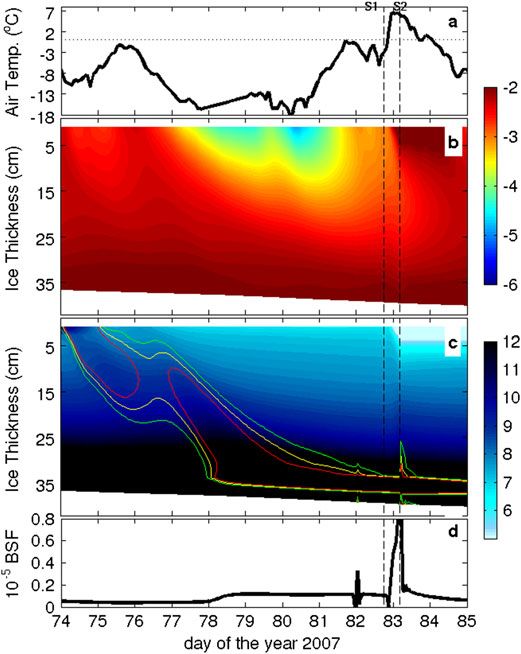
Figure 7. Temporal evolution of (a) in situ air temperature (°C), (b) simulated sea‐ice temperature (°C),
(c) simulated bulk ice salinity with superimposed contours of Rayleigh number equal to 10 (red line), 9.5
(yellow line) and 9 (green line), and (d) simulated basal salt flux (BSF; kg m−2s−1]). The vertical dashed
lines denote the two salinity events (S1 and S2).
443JARDON ET AL.: FULL‐DEPTH DESALINATION OF SEA ICE
of the ice, which reaches a near surface maximum of ~−1.9° the basal salt flux associated with the flushing episode (from
C during S2. The temperature of the ice is unfortunately not day 83 to day 84) leads to a mass of salt of 0.3kgm−2, giving
available at the time of this simulation to assess the accuracy a seawater anomaly of 0.15, comparable with the magnitude
of the model, as it took several days after deployment for the of S2.
hole to refreeze (thermistors located below t5 and t6 [45] Finally, in order to test the impact of initial condi-
shown in Figure 6 all measure seawater temperature). tions, additional simulations with initial salinities Si(t0) equal
Nevertheless, the model has already been compared against to 6, 7, 8, and 9 were performed. Brine convection over the
in situ thermal measurements in previous work [Vancoppenolle entire 40cm ice column occurs for an initial Si of at least
et al., 2007]. 8 (not shown), as predicted by the theoretical analysis
[42] The simulated Si and basal salt flux are shown in (Figure 1b). As in our reference run with Si(t0)=10, these
Figures 7c and 7d, respectively, starting on day 74. The peak are characterized by a supercritical Ra region that reaches
in the salt flux on day 83 (Figure 7c), synchronous with S2, the ice bottom. The minimal salinity of 8 required for
which we previously attributed to flushing, is striking. The convection is consistent with the value of 8.5 measured by
model supports that flushing happens, as confirmed by the Skogseth et al. [2004].
amount of snow melted in the model (not shown), and the
maximal near‐surface desalination (Figure 7c). Interestingly,
immediately after episode S2, the uppermost ice layer 5. Summary and Concluding Remarks
becomes impermeable on day 83.17 owing to the input of [46] In this contribution, based on theory, simulations and
freshwater, while until then the brine volume fraction output observations, we have argued that first‐year sea ice can
by the model shows that the permeability condition (e>5%) undergo substantial desalination when it is warm enough,
was satisfied throughout the full depth of the ice (not and well before summer melt, through gravity drainage pro-
shown). This closure of the brine network at the surface gressing throughout the full thickness of the ice. This cascade
explains why flushing stops rapidly, both in the model and of brine is triggered when ice temperature exceeds a threshold
in observations. depending on thickness and bulk salinity. This condition
[43] In addition to this signal, and quite remarkably, stems from a theoretical analysis (section 2) based on the
Figure 7c shows a desalination starting on day 77 and pro- porous‐medium Rayleigh number, Ra. The latter describes
gressing downward from the top of the ice, similar to that the propensity of brine convection, which occurs when Ra
discussed in the idealized simulations of section 3. It occurs reaches a critical value of Rac ≈10. Ra is proportional to the
in the wake of the Ra=Rac contour, hence triggered by potential energy and to the cube of porosity. Both terms
gravity drainage. The Rac contour reaches close to the ice respond to temperature changes but in an opposite way. Cold
bottom as of day 78, the time at which the basal brine release temperatures enhance potential energy of brine while reducing
gradually increases (Figure 7d). In contrast to the observa- porosity. From these competing effects, it appears that convec-
tions, there is therefore no sporadic increase in the ice‐ocean tion can develop over the entire ice only within a specific
salt flux, which instead gradually increases, except for a temperature range. Indeed, expressing Ra as a function of Ti,
small burst on day 82 associated with a convective event the bundle of Ra(Ti) curves (for different Si and hi) all show
confined within a few centimeters above the ice bottom the same variation, increasing with Ti until reaching a maxi-
associated with the isoline Ra=9. For such values, the model mum before decreasing abruptly. Therefore, by imposing a
indeed starts mimicking brine convection since, as explained threshold Ra=Rac, we define a temperature range [T0,T1]
in section 3, the transition of Dσ(Ra) around Ra=10 is con- outside of which convection is impossible.
tinuous (hyperbolic tangent) and the vertical salt diffusivity [47] Convection will therefore be possible over the entire
is therefore already much larger than the molecular value. ice thickness once its surface temperature exceeds the
In the model, the overall gradual release of salt in the model threshold T0(Si,hi). There is thus some similarity in this
may be an artifact of the diffusive formulation of convection mechanism with the critical thickness required for the onset
(3), where Ra and thus Dσ(Ra) are computed locally at each of convection in growing ice, as evidenced in laboratory
time step. Thus, near the ice base, a supercritical Ra is hardly experiments [Wettlaufer et al., 1997a]. In the latter case,
reached despite the inflow of salty brine from above, because however, it is the increase in the brine's potential energy that
the elevation tends to zero. Contrary to the flushing episode triggers convection; while in the former, it is the decrease in
S2, the simulation fails to reproduce exactly the S1 peak dissipated energy as the temperature increases which is at
apparent in Figure 4, but quite importantly shows that salt play. The value of the temperature threshold T0 is conve-
has accumulated near the ice base (gradually rejected by niently reported in Figure 1b for different bulk salinities
diffusion) owing to gravity drainage during the few days and ice thicknesses. Additionally, this figure shows that this
preceding this event, making gravity drainage the likely expla- convection threshold is well above the temperature warrant-
nation. In this respect, the decrease in salinity that preceded S1 ing sea‐ice permeability (corresponding to e>5%).
(Figure 4) could be interpreted as the trailing edge of a preced- [48] The theoretical argument is supported by idealized
ing sporadic salt rejection. simulation from a 1‐D sea‐ice model with advanced salt
[44] Quantitatively, an integration of the basal salt flux dynamics [Vancoppenolle et al., 2010], where the air temper-
from day 78 to day 83 (occurrence of S1) yields a mass of ature used in the forcing is adjusted to control the ice temper-
0.7kgm−2 of salt rejected (not shown), which translates to ature. Remarkably, simulations show a rapidly developing
a seawater salinity anomaly of 0.7/hmix, where hmix is the cascade of brine through the entire ice layer, yielding a peak
depth in meters of the water layer over which the salt is being in the ice‐ocean salt flux. Sea ice desalinates in this way
mixed. For hmix =2m, we get an anomaly of 0.35 in good by ~3.5. This cascade occurs only when surface ice temper-
agreement with the magnitude of S1. Likewise, integrating ature is warm enough, as posited by theory. The simulation
444JARDON ET AL.: FULL‐DEPTH DESALINATION OF SEA ICE
further reveals that this brine cascade is associated with a increases approximately linearly with Ra, for supercritical
supercritical Rayleigh number, an unambiguous signature Ra up to 60.
of gravity drainage. [53] While they motivated the present analysis, these
[49] Gravity drainage has often been discussed as a winter- serendipitous observations are not complete enough to provide
time desalination mechanism, as opposed to flushing by melt- an indisputable proof of desalination caused by full‐depth
water in summertime. However, in winter, cold temperatures convection, as other possible explanations cannot be totally
enhance potential energy, while convection is efficiently ruled out in the absence of direct measurements within the
opposed by the reduced porosity, so that gravity drainage is ice. These observations can therefore only be viewed as a
restricted to the bottom layers of the ice as seen in the observa- possible example, prompting further analysis of existing
tions of Trodahl et al. [2000] or Pringle et al. [2007]. databases or future dedicated field experiments.
[50] There are only a few observations of desalination in [54] In this respect, the substantial brine release observed in
warming ice, however, which pertain to the existence of the warming ice by Widell et al. [2006] is noteworthy. It, however,
full‐depth convection mechanism discussed here. Pringle appeared to be correlated with the ocean‐ice heat flux, and
et al. [2007] discussed one convective episode developing these authors argued that warm water could prevent refreezing
over 0.8m in 1.30m thick warmer ice, but it was apparently of brine channels, maintaining convection. This mechanism
confined to the ice interior and did not lead to significant brine does not seem at play in our observations, in which no heat
release [Backstrom and Eicken, 2006]. The downward dis- is available from the ocean. Likewise the ocean‐ice heat flux
placement of entrapped brine through the ice in warm condi- plays no role in the mechanism reported here.
tions had also been reported earlier by Kovacs [1996]. He [55] Ice rejects most of its salt during growth. Our analyses
presented these observations in terms of a salinity migration suggest that it loses a substantial fraction of the remnant salt
wave, the amplitude of which diminishes with depth. This immediately after the winter growth season, once the ice
may well be a mechanism similar to the process presented in becomes warm enough to exceed the temperature threshold
this paper; however, no evidence of substantial brine rejection needed to trigger convection through the entire ice column.
out of the ice was reported. Also, from Doronin and Kheisin As this sequence of atmospheric conditions is fairly general,
[1975] field work, such a migration wave was reported to this rapid desalination process is likely to hold for large spatial
migrate downward at about 0.8cm/day, allowing the relative scales in the Arctic.
salinity maximum in the 1.20m thick ice to drop by 17cm in [56] Such full‐depth convective events could be important
23days. This number is, however, much slower than the in regard to the material and gas exchanges at the ocean‐ice‐
mechanism discussed here. atmosphere interface. First, in spring, nutrients are easily
[51] In Storfjorden (Svalbard) in March 2007, we fortu- exhausted by growing ice algae. In this case, any full‐depth
itously recorded two intriguing salinity bursts 1.4m below convection event would replenish nutrients by mixing
the 40cm thick ice, during a warm storm. The first and most nutrient‐rich seawater with nutrient‐depleted brine within
intense seawater salinity anomaly reached 0.41, while the the ice. In turn, this would promote further algal growth
second peaked at 0.21, 10h later. A bundle of evidence, [see Vancoppenolle et al., 2010 for a discussion]. This is
based on data analysis and simulations with the 1‐D halo‐ consistent with observations of the colonization of inner ice
thermodynamic sea‐ice model forced with observed atmo- by algae in late spring (Zhou et al., Brine dynamics across
spheric conditions, suggests that the brine release signals seasons traced by sea‐ice biogeochemistry, manuscript in
are consistent with gravity drainage for the first salinity preparation, 2013). In addition, full‐depth convection would
outburst and caused by the flushing of brine by meltwater enhance gas exchange throughout the sea ice, which has been
for the second (section 4). Regarding the flushing episode, observed in spring for CO2 [e.g., Geilfus et al., 2012].
the timing of the brine rejection in the model and observa- However, because of the sporadic nature of the simulated con-
tions remarkably matches. The model also does simulate a vective events, we argue that those would be hard to detect in
cascade of salt within the ice caused by gravity drainage nature using ice core‐based salinity and temperature measure-
(Figure 7c), starting several days earlier, but reaching the base ments. Sea‐ice cores give only a snapshot of variables that are
of the ice approximately when the first salinity anomaly is highly time dependent.
recorded. This episode of gravity drainage occurs throughout [57] Finally, the frequency of full‐depth convective events
the entire ice, reducing the bulk salinity by 3 (observations is likely to increase in the future Arctic Ocean. In the 20th
suggest a loss ranging between 1.5 and 11.2 assuming century, the Arctic was dominated by old, relatively fresh,
different mixing depths). However, the simulation yields a multi‐year ice. Recent observations and climate projections
smooth increase in the basal salt flux over several days, while indicate that a transition toward a more saline first‐year ice
the observed brine release is sporadic. Among possible pack is occurring [Holland et al., 2006; Maslanik et al.,
reasons for this discrepancy is the model formulation of salt 2007; Vancoppenolle et al., 2009]. Recent observations by
dynamics, in particular the representation of convection as a Maslanik et al. [2011] indicate that first‐year ice already
diffusive process, although the full‐depth convective episode accounts for 55% of the total sea‐ice extent in spring. Only
of the idealized simulation leads to a relatively sharp pulse in salty first‐year ice should be prone to full‐depth convective
the basal flux. Additionally, uncertainties in forcings probably events. Therefore, more first‐year ice means more episodes
contribute to timing differences. of intense and sporadic ice‐ocean salt rejection. Those
[52] Finally, the limits of a 1‐D model should also be episodes would increasingly affect the upper Arctic Ocean,
underlined, since once the ice has reached a critical thick- especially in spring, when the seasonal warming of sea ice
ness, the drainage process is dominated by brine channels. occurs. Those episodes could even perturb the vertical stability
Recent theoretical works by Wells et al. [2011] find that of the upper ocean, deepen and thus warm the mixed layer just
convection controlled by brine channels yields a flux that before melt onset, intensify the ocean‐to‐ice heat flux, as well
445You can also read