Gravity-wave-induced cross-isentropic mixing: a DEEPWAVE case study
←
→
Page content transcription
If your browser does not render page correctly, please read the page content below
Research article
Atmos. Chem. Phys., 23, 355–373, 2023
https://doi.org/10.5194/acp-23-355-2023
© Author(s) 2023. This work is distributed under
the Creative Commons Attribution 4.0 License.

                Gravity-wave-induced cross-isentropic mixing:
                          a DEEPWAVE case study
       Hans-Christoph Lachnitt1 , Peter Hoor1 , Daniel Kunkel1 , Martina Bramberger2 , Andreas Dörnbrack3 ,
            Stefan Müller1,a , Philipp Reutter1 , Andreas Giez3 , Thorsten Kaluza1 , and Markus Rapp3
                   1 Institute for Atmospheric Physics, Johannes Gutenberg University Mainz, Germany
                            2 NorthWest   Research Associates, Boulder Office, Boulder, CO, USA
             3 Institute of Atmospheric Physics, German Aerospace Center (DLR) Oberpfaffenhofen, Germany
                                     a now at: enviscope GmbH, Frankfurt/Main, Germany

                           Correspondence: Hans-Christoph Lachnitt (hlachnit@uni-mainz.de)

                                    Received: 13 June 2022 – Discussion started: 6 July 2022
                     Revised: 13 December 2022 – Accepted: 14 December 2022 – Published: 10 January 2023

      Abstract. Orographic gravity waves (i.e., mountain waves) can potentially lead to cross-isentropic fluxes of
      trace gases via the generation of turbulence. During the DEEPWAVE (Deep Propagating Gravity Wave Experi-
      ment) campaign in July 2014, we performed tracer measurements of carbon monoxide (CO) and nitrous oxide
      (N2 O) above the Southern Alps during periods of gravity wave activity. The measurements were taken along two
      stacked levels at 7.9 km in the troposphere and 10.9 km in the stratosphere. A detailed analysis of the observed
      wind components shows that both flight legs were affected by vertically propagating gravity waves with mo-
      mentum deposition and energy dissipation between the two legs. Corresponding tracer measurements indicate
      turbulent mixing in the region of gravity wave occurrence.
         For the stratospheric data, we identified mixing leading to a change of the cross-isentropic tracer gradient of
      N2 O from the upstream to the downstream region of the Southern Alps. Based on the quasi-inert tracer N2 O, we
      identified two distinct layers in the stratosphere with different chemical composition on different isentropes as
      given by constant potential temperature 2. The CO–N2 O relationship clearly indicates that irreversible mixing
      between these two layers occurred. Further, we found a significant change of the vertical profiles of N2 O with
      respect to 2 from the upstream to the downstream side above the Southern Alps just above the tropopause. A
      scale-dependent gradient analysis reveals that this cross-isentropic gradient change of N2 O is triggered in the
      region of gravity wave occurrence.
         The power spectra of the in situ measured vertical wind, 2, and N2 O indicate the occurrence of turbulence
      above the mountains associated with the gravity waves in the stratosphere. The estimated eddy dissipation rate
      (EDR) based on the measured three-dimensional wind indicates a weak intensity of turbulence in the stratosphere
      above the mountain ridge. The 2–N2 O relation downwind of the Alps modified by the gravity wave activity
      provides clear evidence that trace gas fluxes, which were deduced from wavelet co-spectra of vertical wind and
      N2 O, are at least in part cross-isentropic.
         Our findings thus indicate that orographic waves led to turbulent mixing on both flight legs in the troposphere
      and in the stratosphere. Despite only weak turbulence during the stratospheric leg, the cross-isentropic gradient
      and the related composition change on isentropic surfaces from upstream to downstream of the mountain unam-
      biguously conserves the effect of turbulent mixing by gravity wave activity on the trace gas distribution prior to
      the measurements. This finally leads to irreversible trace gas fluxes across isentropes and thus has a persistent
      effect on the upper troposphere and lower stratosphere (UTLS) trace gas composition.

Published by Copernicus Publications on behalf of the European Geosciences Union.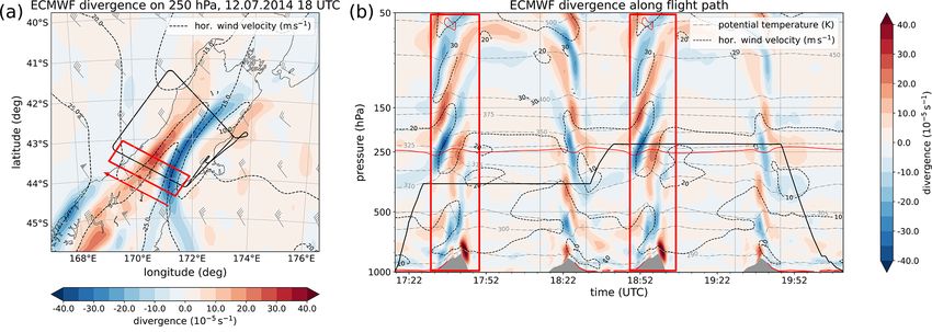
356                                                          H.-C. Lachnitt et al.: Gravity wave induced cross-isentropic mixing

1   Introduction                                                        The effect of orographic waves on tracer transport and
                                                                     mixing and the emerging tracer redistributions has been dis-
Orographic gravity waves affect the large-scale stratospheric        cussed frequently (Schilling et al., 1999; Heller et al., 2017;
circulation and play an important role in determining the            Moustaoui et al., 2010; Zhang et al., 2015; Podglajen et al.,
thermal and dynamical structure of the atmosphere (e.g.,             2017; Grubišić et al., 2008; Woiwode et al., 2018). Obser-
Smith et al., 2008; Fritts and Alexander, 2003; Kim et al.,          vational studies mainly addressed the analysis of local kine-
2003; Alexander and Grimsdell, 2013; Rapp et al., 2021).             matic fluxes using the covariance of the local vertical winds
Many observations of stratospheric gravity waves are based           and the tracer fields (Shapiro, 1980; Schilling et al., 1999).
on satellite observations (e.g., Alexander et al., 2008; Geller      Based on airborne observations in a tropopause fold, Shapiro
et al., 2013; Ern et al., 2018). However, in the upper tropo-        (1980) identified ozone and particle fluxes in regions of tur-
sphere and lower stratosphere (UTLS), observations of grav-          bulence and shear. They estimated vertical turbulent tracer
ity waves from aircraft and balloon soundings are essential          fluxes by approximating the change of the mean tracer flux
for process studies beyond the resolution of satellites (e.g.,       by the divergence of the vertical turbulent tracer flux. This
Podglajen et al., 2016; Krisch et al., 2017; Wright and Ban-         approach has been used to derive mountain-wave-induced
yard, 2020; Rapp et al., 2021). Gravity waves may locally            tracer fluxes using the flux divergence approach between
lead to the generation of convective instabilities (Lane and         two flight legs (with altitude differences of typically 1000 m)
Sharman, 2006) or dynamical instability induced by vertical          providing evidence for a vertical flux of carbon monoxide
shear of the horizontal wind (Panofsky et al., 1968; Kunkel          (Schilling et al., 1999) or water vapor (Heller et al., 2017).
et al., 2014; Söder et al., 2021). Both types of instability            Direct observations of gravity-wave-induced cross-
may lead to the occurrence of turbulence, particularly when          isentropic tracer mixing are sparse, since this requires
wave breaking occurs, potentially leading to mixing of trace         high-resolution measurements of passive tracers (i.e., tracers
species (Pavelin et al., 2002; Whiteway et al., 2003).               without chemical or microphysical sources or sinks) exactly
   The tropopause as a central feature of the UTLS acts as a         in the region of turbulence associated with these waves.
dynamical barrier for transport of species and the formation         Kinematic fluxes based on the covariance of the local
of trace gas gradients at the tropopause (e.g., Gettelman et al.,    vertical wind and the passive tracers are not necessarily
2011; Woiwode et al., 2018; Hoor et al., 2002; Pan et al.,           irreversible. Analysis of the relation between tracer mixing
2004). To overcome this dynamical barrier, diabatic pro-             and orographic wave activity (Moustaoui et al., 2010;
cesses are required, which can be associated with radiation-         Mahalov et al., 2011) highlighted the importance of the
driven processes or phase transitions of water. Wave breaking        local tropopause structure for the interpretation of fluxes.
of planetary waves and stirring may cause a scale breakdown          On the basis of in situ observations, Moustaoui et al. (2010)
in the tracer structure with subsequent mixing of tracers by         concluded that the layers within the UTLS including the
molecular diffusion (e.g., Balluch and Haynes, 1997).                tropopause may behave like material surfaces and that
   In addition, turbulence produced by wave breaking and             vertical displacements are largely reversible despite the oc-
wind shear above the tropopause (Shapiro, 1980; Söder et al.,        currence of gravity waves. They further pointed out that the
2021; Kaluza et al., 2021, 2022; Lilly et al., 1974) provides        observed tracer characteristics are the result of a non-linear
such another efficient diabatic process. It leads to cross-          interaction between synoptic-scale waves modulated by
isentropic mixing and thus irreversible trace gas exchange           shorter gravity waves, leading first to reversible transport
at the tropopause. We will use the term cross-isentropic to          and tracer mixing.
emphasize the irreversible (entropy changing i.e., potential            On the basis of observed passive tracers, this study pro-
temperature changing and therefore diabatic) nature of this          vides evidence that the breaking of mountain waves can lead
process. Further, the term cross-isentropic allows us to dis-        to tracer redistribution in the tropopause region by cross-
tinguish from quasi-isentropic mixing. The latter is driven by       isentropic mixing. We investigate how orographic gravity-
synoptic and planetary waves leading to stirring and mixing          wave-induced turbulence leads to a persistent effect on the
best approximated along isentropes.                                  UTLS composition downwind of the turbulent mixing re-
   Irreversible (entropy changing) processes lead to an ir-          gion.
reversible redistribution of tracers which must therefore be            The paper is organized as follows: we will first describe the
cross-isentropic providing a tracer flux crossing isentropes.        measurements and techniques; we will briefly introduce the
Turbulence at the tropopause can be generated by a num-              DEEPWAVE (Deep Propagating Gravity Wave Experiment)
ber of processes, e.g., strong shear at the jet streams (e.g.,       project and the meteorological conditions during the flight.
Kaluza et al., 2021), convection (Wang, 2003; Mullendore             Section 3 will focus on the observations and the identifica-
et al., 2005; Homeyer et al., 2017) or frontal uplift leading to     tion of mixing from tracer measurements of N2 O and CO. In
strong vertical convergence of the horizontal wind (Panofsky         Sect. 4, we will identify the effect of cross-isentropic mixing
et al., 1968; Söder et al., 2021) and the generation of gravity      and use different methods to show that gravity-wave-induced
waves (e.g., Whiteway et al., 2003; Wang, 2003).                     turbulence and subsequent mixing has affected the observed
                                                                     tracer–2 relationship with a persistent impact on the compo-

Atmos. Chem. Phys., 23, 355–373, 2023                                                   https://doi.org/10.5194/acp-23-355-2023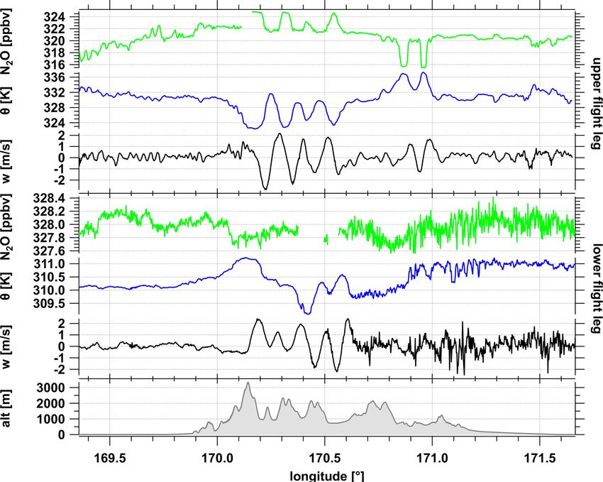
H.-C. Lachnitt et al.: Gravity wave induced cross-isentropic mixing                                                        357

sition in the downstream side of the mountain ridge. The re-     inertial system (Mallaun et al., 2015). For the vertical wind
sults will be analyzed for cross-isentropic transport followed   component, an uncertainty of ± 0.3 m s−1 is estimated. The
by a discussion.                                                 true static air temperature is provided with a measurement
                                                                 uncertainty of ± 0.5 K.
2     Data and methods
                                                                 2.3   Meteorological analysis data
2.1    Campaign and instrumentation
                                                                 To support our analysis and obtain information of the syn-
The measurements were performed in the frame of the              optic background, we used ECMWF (European Center for
DEEPWAVE (Deep Propagating Gravity Wave Experiment)              Medium-Range Weather Forecast) IFS (Integrated Forecast-
mission in summer 2014 over New Zealand (Fritts et al.,          ing System) operational analysis data. The data are available
2016; Gisinger et al., 2017). The project combined a com-        every 6 h and have been interpolated on a horizontal grid with
prehensive set of ground-based measurements as well as air-      a spacing of 0.125◦ for our analysis. In total, the model has
borne measurements by the NSF (National Science Foun-            137 vertical hybrid sigma-pressure levels from the surface up
dation)/NCAR (National Center for Atmospheric Research)          to 0.01 hPa. The vertical grid spacing is about 300 m in the
Gulfstream GV HIAPER (High-performance Instrumented              tropopause region. For our analysis, the model data are lin-
Airborne Platform For Environmental Research) and Ger-           early interpolated in time and space onto the location of the
man DLR (Deutsches Zentrum für Luft- und Raumfahrt)              flight track.
Dassault Falcon 20E aircraft. Airborne measurements were
carried out from Christchurch during June and July 2014
that covered the UTLS and provided remote-sensing data           2.4   Wavelet analyses
up to 80 km. The majority of the measurements focused on         The wavelet analysis is a tool for the spectral analysis of
the Southern Alps to study the evolution of mountain waves       time series data (Torrence and Compo, 1998). The advan-
from their source to the breaking regions in the mesosphere.     tage over Fourier analysis is the ability to show information
The two aircraft partly performed coordinated flights in the     in time and frequency space. Wavelet analysis has frequently
tropopause region to study the propagation and potential dis-    been used for the analysis of gravity waves (e.g., Bram-
sipation of gravity waves in this region. On 12 July, which is   berger et al., 2017; Zhang et al., 2015; Woods and Smith,
the day of the analysis in this paper, no HIAPER flight was      2011, 2010). The wavelet basis function which we use in this
performed.                                                       study is the Morlet wavelet with non-dimensional frequency
                                                                 ω0 = 6 as defined in Torrence and Compo (1998). To reveal
2.2    Aircraft measurements                                     periods with significant wavelet power, we determined the
                                                                 95 % confidence level (which is equivalent to the 5 % sig-
Tracer measurements of N2 O and CO were performed using          nificant level) in the respective analyses below as described
the University MAinz Quantum Cascade Absorption Spec-            in Torrence and Compo (1998). The wavelet cospectrum can
trometer (UMAQS, Müller et al., 2015) onboard the DLR            be used to analyze spectral characteristics of turbulent fluxes
Falcon. The instrument consists of a Herriott cell with a path   (e.g., Mauder et al., 2007; Zhang et al., 2015). The wavelet
length of 36 m. We detected N2 O and CO at wavenumbers of        cospectrum W AB of 2 time series A and B with the wavelet
2002.75 and 2003.16 cm−1 , respectively, by scanning with a      transforms W A and W B is defined as the real part of the
frequency of 9 kHz across the absorption lines at a cell pres-   cross-wavelet transformation:
sure of 50 hPa. The UMAQS is capable of simultaneously                         n                o
measuring the species N2 O and CO reported here as volume        WnAB (s) = < WnA (s)WnB∗ (s) ,                              (1)
mixing ratios in parts per billion per volume (ppbv) with a
temporal resolution of 10 Hz, ultimately limited by the flow     where the asterisk denotes the complex conjugation, n a local
speed and purging time of the cell. We apply in situ calibra-    time index and s the wavelet scale (Torrence and Compo,
tions using secondary standards of compressed ambient air        1998; Liu et al., 2007).
which are traced to primary standards of NOAA (National             Another tool which we use in this study is the wavelet co-
Oceanic and Atmospheric Administration) prior and after the      herence R 2 . It represents the covariance between the 2 time
campaign. The precision of the data (given here for the 1 Hz     series A and B and can be used to identify frequency and
averaged data) is in the order of 0.05 ppbv (1 standard devia-   time intervals with strong and weak coherence between the
tion σ ) for N2 O and CO, respectively.                          variations of the two data sets. The wavelet coherence is de-
   We further use measurements of the basic atmospheric          fined as
state parameters at 10 Hz provided by the Falcon aircraft
(Krautstrunk and Giez, 2012). The three-dimensional wind                                S s −1 WnAB (s)
                                                                                                        2
is deduced from a five-hole gust probe located in the nose       Rn2 (s) =                                    ,         (2)
                                                                                             2                 2
boom providing true air speed and the ground speed from the                  S s −1   WnA (s) · S s −1 WnB (s)

https://doi.org/10.5194/acp-23-355-2023                                                Atmos. Chem. Phys., 23, 355–373, 2023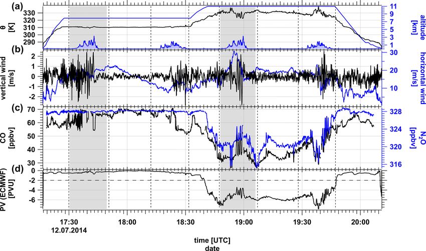
358                                                        H.-C. Lachnitt et al.: Gravity wave induced cross-isentropic mixing

where S is a smoothing operator in space and time (for fur-        surement of gravity waves. Here, we focus on the flight legs
ther details, see e.g., Torrence and Compo, 1998; Grinsted         parallel to the wind and orthogonal to the mountains of re-
et al., 2004; Jevrejeva et al., 2003).                             search flight FF09.

3     Observations and meteorological situation during             3.2   Time series analysis of FF09
      FF09                                                         During flight FF09 on 12 July 2014, the flight legs were al-
                                                                   most parallel to the horizontal wind and directed almost per-
3.1    Meteorological situation on 12 July 2014
                                                                   pendicular to the Southern Alps. Pronounced fluctuations of
In this study, we focus on research flight FF09 of the Falcon      the vertical wind occurred above the Southern Alps at each
aircraft on the 12 July 2014 starting at 17:15 to 20:15 UTC        flight leg crossing the mountain ridge (Fig. 2).
(Fig. 1). The goal of this flight was to investigate the dynam-       The tropopause was crossed around 18:40 UTC, as indi-
ical and chemical structure of the atmosphere in the vicin-        cated by the sharp decrease of the N2 O volume mixing ratio
ity of tropopause during a mountain wave event (Gisinger           and the analyzed potential vorticity (PV) interpolated along
et al., 2017; Smith et al., 2016). As can be seen in Fig. 1, a     the flight path. Particularly in the regions of strong variability
rectangular pattern was flown clockwise to measure differ-         of the vertical wind, 2, N2 O and CO show enhanced variabil-
ent wave responses in the northern and middle part of the          ity and strong fluctuations during the stratospheric part of the
Southern Island of New Zealand at two different pressure           flight.
levels (330 and 260 hPa, Fig. 1), corresponding to approxi-           The fluctuations of 2 reached an amplitude of 12 = 9 K
mately 7.9 and 10.9 km pressure altitude. The time between         (Fig. 2). Corresponding oscillations of the vertical wind ve-
two vertically stacked legs at the same location was 75 min        locity reached 5 m s−1 peak to peak with associated variabil-
(Fig. 2).                                                          ity of N2 O in the order of 4 ppbv mirroring the oscillations
   According to Gisinger et al. (2017), the synoptic situa-        of potential temperature during both flight sections parallel
tion can be characterized by a trough located west of New          to the wind. These features occurred above the mountains
Zealand with a weak surface low located south of the is-           where the meteorological analysis shows a slight altitude
lands causing northwesterly winds in the troposphere (TNW          variability of the dynamical tropopause (−2 PVU, Fig. 1).
regime, Fig. 2e in Gisinger et al., 2017). In the upper level
at 250 hPa at the eastern side of the approaching upper level      3.3   Orographic waves during FF09
trough, a weak gradient of the geopotential height led to a
northwesterly flow with moderate horizontal winds of typi-         The flight sections of the two southern legs were strongly af-
cally 20 m s−1 along the southern flight legs (with 30 m s−1       fected by orographic waves (Fig. 3). Both legs show strong
above the mountain ridge). The tropopause became rela-             fluctuations of the vertical wind component w and the poten-
tively flat in the region and at the time of the measurements      tial temperature 2 with amplitudes of 2.5 m s−1 and 4.5 K,
(Fig. 1b). These conditions led to the excitation of moun-         respectively. The passive tracer nitrous oxide (N2 O) indicates
tain waves and generated varying and moderate gravity wave         corresponding fluctuations at the upper level in the strato-
responses over the South Island (Gisinger et al., 2017). Fig-      sphere. At the lower level, N2 O shows a weak variability.
ure 1a shows the divergence of the ECMWF horizontal wind           Due to its virtually constant abundance in the troposphere,
at 250 hPa at 18:00 UTC which roughly corresponds to the           N2 O does not show corresponding oscillations to w and 2
time of flight. The vertical cross section interpolated in time    between 170.1–170.7◦ E. However, its variability does in-
and space along the flight path shows a wave pattern above         crease downwind of the mountains similar to w and 2, indi-
the mountain ridge indicating the excitation and propagation       cating the occurrence of turbulence. At the upper level, such
of orographic gravity waves, which propagate deep into the         turbulence is not prominent, although the fluctuations of 2,
stratosphere (Fig. 1b).                                            w and N2 O (Fig. 3) are indicative of at least a potential kine-
   It is evident from Fig. 1b that the upper flight leg at         matic flux of N2 O, with only weakly pronounced small scale
about 10.9 km is just above the dynamical tropopause. A            variability of w0 (we defined the primed quantities according
close inspection of Fig. 1b reveals an almost constant alti-       to Eq. 4).
tude of the dynamical tropopause along the flight path with-          Before studying tracer transport and mixing, we ana-
out strong horizontal gradients or folds in the region of our      lyzed the dynamical properties of the orographic waves. The
measurements. The flat dynamical tropopause structure is           binned energy spectra of the vertical wind and the hori-
mirrored by the ozone distribution from ERA5 data (not             zontal wind speed VH are shown in Fig. 4 for the south-
shown), which shows a rather homogeneous distribution at           ern flight legs crossing the mountains. Both legs show pro-
2 = 330 K (approximately flight altitude) and notably also         nounced peaks in the w spectra at about 10 km horizon-
upwind of the region of our measurements.                          tal wavelength. The vertical turbulent kinetic energy was
   As mentioned above, a rectangular flight pattern at two dif-    larger in the lower leg (w02 = 0.70 m2 s−2 ) than in the up-
ferent altitudes (7.9 and 10.9 km) was chosen for the mea-         per leg (w02 = 0.53 m2 s−2 ), where the overline denotes the

Atmos. Chem. Phys., 23, 355–373, 2023                                                 https://doi.org/10.5194/acp-23-355-2023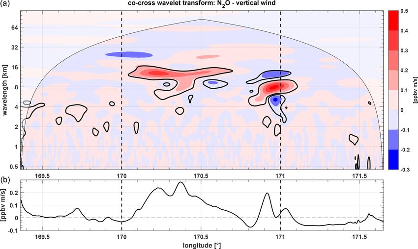
H.-C. Lachnitt et al.: Gravity wave induced cross-isentropic mixing                                                                       359

Figure 1. Divergence of the ECMWF horizontal wind during the time of flight (a) at 250 hPa and (b) as vertical cross section along the flight
track indicating the signature of gravity waves over the Southern Alps. The solid red line denotes the −2 PVU isoline and the solid black
line denotes the flight track. The dashed black lines denote contours of the horizontal wind velocity (10, 15, 20, 25 m s−1 in (a) and 10, 20,
30 m s−1 in (b)) and the dashed gray lines in (b) denote contours of potential temperature. Regions of interest are marked by red rectangles
and the red arrow in (b) indicates the clockwise flight direction.

Figure 2. Time series of (a) potential temperature 2 from the measurements (black), altitude (blue) above surface elevation (filled blue),
(b) vertical wind (black), horizontal wind (blue), (c) N2 O (blue) and CO (black) volume mixing ratios and (d) ECMWF potential vorticity
(PV) interpolated along the flight track. Light gray boxes indicated the tropospheric and stratospheric flight section for the detailed mixing
analysis. Vertical dashed lines mark turning points of the aircraft. Surface elevation was interpolated from SRTM15+ data (Tozer et al., 2019).

average over the whole 200 km flight leg. However, the en-                   The situation is different for the horizontal wind spectra
ergy of the lower leg seems to reside in scales smaller than              where the energy is at longer horizontal scales. Only the up-
about 1 km. Therefore, the spectral amplitude associated with             per leg shows a spectral peak at 10 km similar to the one
the mountain waves at horizontal wavelengths of λx = 10 km                in w. Thus, there are two distinct gravity wave modes: one
is smaller at the lower leg, whereas at the upper leg, wave mo-           with a long horizontal wavelength (also partly seen in VH in
tions with λx ≈ 10 km dominate. No vertical energy is found               Fig. 2 around 17:45 UTC) that is a response to the airflow
at larger scales in both legs.                                            over the whole mountain range and one with λx ≈ 10 km.

https://doi.org/10.5194/acp-23-355-2023                                                       Atmos. Chem. Phys., 23, 355–373, 2023
360                                                              H.-C. Lachnitt et al.: Gravity wave induced cross-isentropic mixing

Figure 3. Cross section of the two southern stacked flight legs crossing the Southern Alps (shaded gray regions of Fig. 2) showing N2 O
(green), 2 (blue) and vertical wind w (black) for the upper leg at 10.9 km (top three panels) and the lower leg at 7.9 km with surface elevation
(bottom). Both legs are separated by 75 min in time. The upper leg lies in the lower stratosphere just above the tropopause, the lower leg lies
in the upper troposphere.

The long mode is totally absent in the lower leg and corre-                 An estimate of the vertical momentum flux divergence
sponds well to the rather uniform horizontal wind as shown                based on the values from the stacked flight legs,
in Fig. 2 (17:30–17:50 UTC). This long mode was probably
not fully captured by the limited lengths of the legs as flown                1 ∂            ∂        ∂u
                                                                          −        ρu0 w0 ≈ − u0 w0 =    ,                                  (3)
by the DLR Falcon. The other, shorter mode in the horizontal                  ρ ∂z           ∂z       ∂t
wind spectra is well-developed only in the lower leg. How-
ever, the increase of the spectral variance from the lower leg            yields a deceleration of the zonal flow ∂u/∂t of about
to the upper leg by a factor of 7 from 1.88 to 13.78 m2 s−2               6 m s−1 d−1 . This indicates momentum deposition by dissi-
must be mainly related to the long wave observed there ac-                pating mountain waves most likely occurring in the layer be-
cording to Fig. 4.                                                        tween the lower leg and the upper leg. The slowdown does
   The downstream regions of the lower leg show increased                 not seem to affect the wave-induced increase of horizontal
variances of the vertical wind w 0 at short horizontal wave-              wind in the upper flight leg. Thus, the momentum dissipation
lengths. These enhanced variances might be related to the                 must have occurred between the two flight segments sepa-
increase of small-scale energy as can be seen in the spectra              rated vertically by 3000 m. This argument is supported by the
shown in Fig. 4. The specific zonal momentum fluxes u0 w0                 small-scale signatures found in all wind components down-
(Table 1) are negative above the mountains and their magni-               stream of the coherent waves in the lower leg (see Figs. 2
tude is much larger than up- and downstream. This indicates               and 3). They indicate turbulent modes associated with local
a vertical upward transport of negative horizontal momen-                 instabilities above this level.
tum that is characteristic of vertically propagating mountain                The meridional momentum fluxes v 0 w0 are much smaller
waves.                                                                    than u0 w0 (Table 1) and will not be considered here. The
                                                                          zonal wave energy fluxes u0 p 0 are negative in all segments of
                                                                          both legs (Table 1) and their magnitudes are largest directly
                                                                          over the mountains. Together with the positive vertical wave
                                                                          energy flux w0 p0 , this finding suggests vertically propagating

Atmos. Chem. Phys., 23, 355–373, 2023                                                          https://doi.org/10.5194/acp-23-355-2023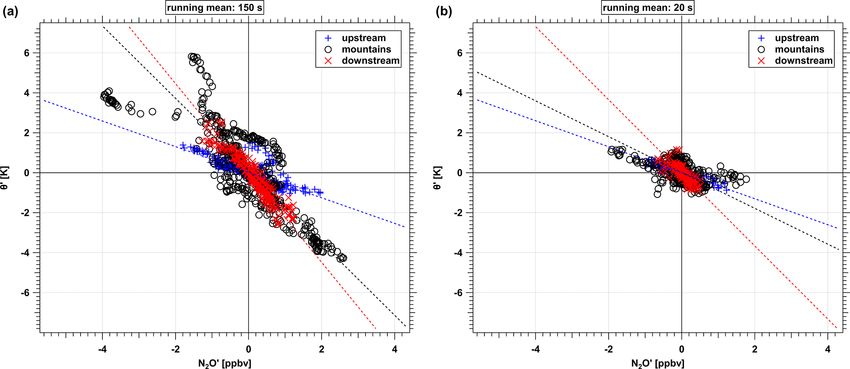
H.-C. Lachnitt et al.: Gravity wave induced cross-isentropic mixing                                                                    361

Figure 4. Binned energy spectra for the vertical wind component w (a, b) and the horizontal wind VH (c, d) from the two southern flight
legs of FF09, which crossed the mountains based on the 10 Hz data (corresponding to flight segments from 17:30–17:50 UTC and 18:47–
19:07 UTC in Fig. 2). The left column shows the lower tropospheric flight track. Thick black lines are results without tapering window, thin
black lines are spectra tapered with a Hanning window.

Table 1. Wave momentum and wave energy fluxes for the two southern legs separated in upstream, downstream and across mountain side
according to Fig. 6.

                                                   Tropospheric leg                        Stratospheric leg
                                        Upstream    Mountain     Downstream    Upstream      Mountain     Downstream

                       u0 w 0 /m2 s−2       0.02        −0.37         −0.18        −0.01        −0.16            0.02
                       v 0 w0 /m2 s−2       0.00        −0.21          0.09         0.01         0.02           −0.02

                       u0 p 0 /W m−2      −0.24        −12.48         −8.72        −0.89       −24.80           −1.52
                       v 0 p0 /W m−2       0.32          7.08          4.91         0.24         3.28            0.84
                       w 0 p0 /W m−2       0.04          4.17          0.07         0.04         1.08            0.02

mountain waves that travel against the mean flow, therefore,            duced in the up- and downstream segments, indicating no
u0 p 0 < 0.                                                             significant vertical wave propagation there.
   It is interesting to note that the vertical wave energy flux
w0 p 0 decreases with height by a factor of 4, which means that
the waves are attenuated as they propagate from the lower leg           3.4    Observation of mixing
to the upper leg. This supports the idea that dissipation must
have occurred in the layer between 7.9 and 10.9 km altitude.            We use tracer–tracer scatter plots of CO and N2 O to investi-
Vertical and horizontal wave energy fluxes are drastically re-          gate if mixing occurred in the region of the enhanced wave
                                                                        activity. Since N2 O has no chemical sink in the atmosphere

https://doi.org/10.5194/acp-23-355-2023                                                     Atmos. Chem. Phys., 23, 355–373, 2023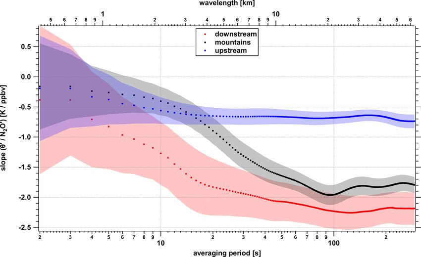
362                                                             H.-C. Lachnitt et al.: Gravity wave induced cross-isentropic mixing

                                                                        stratospheric air is involved. Thus we cannot diagnose mix-
                                                                        ing for the lower leg on the basis of tracer–tracer correlations.
                                                                           However, for the stratospheric legs across the moun-
                                                                        tain ridge during FF09, the scatter plot clearly shows
                                                                        different chemical regimes in the stratosphere (i.e., for
                                                                        N2 O < 326 ppbv, Fig. 5) as indicated by the two differ-
                                                                        ent branches of the two tracers. These two branches indi-
                                                                        cate two distinct air masses within the lower stratosphere
                                                                        which differ in their chemical composition as evident by
                                                                        the different N2 O volume mixing ratios. A detailed anal-
                                                                        ysis (see Fig. 6) shows that the two branches of the cor-
                                                                        relation can be assigned to two distinct potential temper-
                                                                        ature intervals which correspond to two layers of differ-
                                                                        ent chemical composition for 2 > 328.1 K and 2 < 326.3 K.
                                                                        Notably, the data points (marked in green) which fall be-
                                                                        tween the two data clouds (N2 O < 324 ppbv) forming two
                                                                        compact branches (and thus isentropes as given above) con-
                                                                        nect both air masses. The intermediate points thus mark
                                                                        a layer between 326.3 K < 2 < 328.1 K, where the tracer–
Figure 5. Scatterplot of N2 O versus CO for FF09 on 12 July 2014.       tracer diagram indicates mixing between the two branches
The light gray points show the correlation of N2 O and CO for           (green squares in Fig. 5).
the whole flight. For the upper southwestern flight leg from 18:48
                                                                           To put the stratospheric part (i.e., for N2 O < 327 ppbv)
to 19:06 UTC in Fig. 2 (also compare Fig. 6), the data points are
                                                                        of the tracer–tracer data of the scatter plot in a geophysi-
black, blue and green. Black colors indicate potential temperatures
2 > 328.1 K, blue for 2 < 326.3 K. The region between these two         cal and meteorological context, Fig. 6 shows the time series
levels is marked in green. The lower leg lies entirely in the tropo-    of potential temperature and N2 O color coded according to
sphere as indicated by the orange data points of N2 O = 328 ppbv.       the regimes identified from the scatterplot (Fig. 5). The two
                                                                        branches of the correlation can be clearly assigned to differ-
                                                                        ent isentropes separating air masses with different chemical
                                                                        composition. Notably, those points which indicate mixing in
below 25 km and a lifetime of 110 years in the lower strato-            the tracer-tracer scatterplot fall between the distinct layers.
sphere, it is virtually homogeneously distributed in the tro-           As evident from Fig. 6, the region where the chemical com-
posphere, but exhibits a weak vertical gradient in the strato-          position indicates mixing (green) corresponds to the occur-
sphere (Müller et al., 2015). In contrast, CO has a chemical            rence of waves as indicated by strong fluctuations of the ver-
lifetime in the order of weeks to months in the tropopause              tical wind and potential temperature. Therefore, we hypothe-
region. Thus, it shows a sharper gradient at the tropopause.            size that mountain-wave-induced mixing must have occurred
Particularly in the absence of mixing from the troposphere,             in the stratosphere leading to the observed tracer variability
CO would fall to volume mixing ratios of 10–15 ppbv given               as shown above. In the following section, we will therefore
by the balance of CO production from methane oxidation                  focus on the stratospheric flight section across the mountains
and faster CO degradation by OH. Any higher value is in-                from 18:48 to 19:06 UTC as indicated by the gray box in
evitably linked to a contribution of tropospheric air. There-           Fig. 2 if not noted differently.
fore mixing, in the sense of irreversible tracer transfer, can
be detected by comparing CO to any long-lived tracer with
a stratospheric gradient. The approach has been extensively
used to detect tropospheric influence in the stratosphere by            4   Analysis of cross-isentropic mixing
using CO and ozone (O3 ) (e.g., Hoor et al., 2002; Zahn and
Brenninkmeijer, 2003; Pan et al., 2004). Here, we use N2 O              Kinematic fluxes on the basis of the covariance of vertical
instead of O3 since it is purely controlled by atmospheric dy-          wind and tracer variability w 0 χ 0 might provide information
namics in the lower stratosphere due to the absence of local            on the local vertical fluxes. For a correct estimate of an ir-
photochemical sources and sinks.                                        reversible flux, one needs to calculate the flux divergence
   The scatter plot of CO versus N2 O for both southwesterly            (Shapiro, 1980). However, this would require simultaneous
legs of FF09 is shown in Fig. 5. The orographic waves at                measurements of the tracer of interest on two closely stacked
the lower leg appear at almost constant N2 O volume mixing              vertical levels, which cannot be accomplished with one air-
ratios of 328 ppbv. This is due to the fact that in the tropo-          craft (as was the case here). A comparison of the local fluxes
sphere, no gradients of N2 O are present. Therefore, mixing             for the stacked levels is in principle possible. However, due
does not change the N2 O volume mixing ratio as long as no              to the large vertical spacing of 3 km, the potential influence

Atmos. Chem. Phys., 23, 355–373, 2023                                                      https://doi.org/10.5194/acp-23-355-2023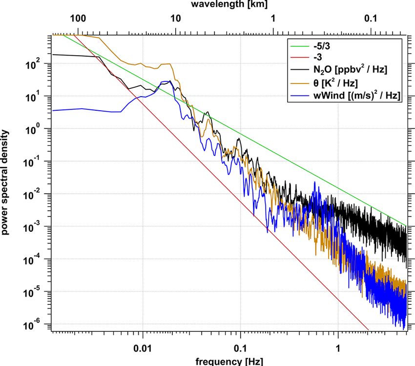
H.-C. Lachnitt et al.: Gravity wave induced cross-isentropic mixing                                                                363

Figure 6. Time series of potential temperature 2 and N2 O for the flight leg around 18:48–19:00 UTC just above the tropopause over the
mountain. Colors indicate two different layers of air masses (black, blue) and a mixed layer in between (green) corresponding to Fig. 5.
Vertical lines mark the upstream (< 170◦ E), above mountain (170–171◦ E), and downstream side (> 171◦ E).

from large-scale horizontal advection could strongly impact           cal control. At the tropopause, N2 O exhibits a change of the
the flux divergence estimates between the two flight levels.          vertical gradient with respect to 2 (∂N2 O/∂2).
   Adiabatic vertical displacements of air masses may simul-             The decrease of N2 O in the lowermost stratosphere with
taneously displace the location of isentropes and tracer iso-         respect to 2 is schematically shown in Fig. 7. For the fol-
pleths, which therefore does not lead to irreversible tracer          lowing analysis, we will use the following conventions: we
transport and mixing at a given location downwind of                  will express the slope as ratio of the anomalies 20 /N2 O0 (ac-
a mountain ridge (i.e., ∂χ /∂2 = const, Moustaoui et al.,             cording to Eq. 4) to be consistent with the profile view (as in
2010). In contrast, cross-isentropic (= diabatic) fluxes must         Figs. 7 and 8). We will apply this convention with 2 in the
change cross-isentropic gradients of species (i.e., ∂χ /∂2)           numerator and N2 O in the denominator throughout the fol-
with respect to potential temperature. Therefore, a change            lowing analyses. We will further use the terminology below.
of tracer gradient (i.e., ∂N2 O/∂2; similar to Balluch and               The term 2–N2 O relation refers to general aspects of their
Haynes, 1997) as a function of 2 downwind of the mountain             relation, the term 20 /N2 O0 ratio (associated with a slope)
is indicative of irreversible cross-isentropic tracer exchange        will be used when referring to the specific measurements.
which might have occurred above the mountain ridge. In a              A change of this ratio is directly linked to the change of the
Lagrangian sense, the occurrence of turbulence and turbu-             vertical gradient with respect to 2 (∂N2 O/∂2).
lent mixing acts as a source of tracer at a given isentrope,             A schematic of our hypothesized relation of 2 and N2 O is
if the background tracer gradient changes with height in the          shown in Fig. 7 which shows the evolution of the N2 O profile
inflow region (e.g., at the tropopause). We therefore investi-        for a flow over a mountain assuming an effect of gravity-
gated whether tracer gradients with respect to potential tem-         wave-induced cross-isentropic mixing on the N2 O profile.
perature 2 were changed due to the occurrence of gravity-             The upstream side represents the unperturbed background
wave-induced turbulence leading to cross-isentropic mixing            N2 O profile. Above the mountain, orographic-wave-induced
by comparing local tracer profiles upstream and downstream            turbulence may occur which could potentially change the
of the mountains (∂χ /∂2|up 6 = ∂χ /∂2|down ).                        vertical gradient of N2 O with respect to 2 at the tropopause.
   In particular, the gradient change of the conservative tracer      This effect of irreversible mixing is schematically depicted
N2 O at the tropopause is perfectly suited to test our hy-            by the gray shading in Fig. 7. Since ∂N2 O/∂2 changes at
pothesis that gravity-wave-induced turbulence led to cross-           the tropopause, the upstream relation between 2 and N2 O
isentropic mixing. Since N2 O in the lowermost stratosphere           can be modified by turbulent mixing which will change the
is not affected by local chemistry, it is purely under dynami-        relation of the N2 O profile with respect to 2. As a result of
                                                                      the irreversible diabatic process, the downstream side shows

https://doi.org/10.5194/acp-23-355-2023                                                  Atmos. Chem. Phys., 23, 355–373, 2023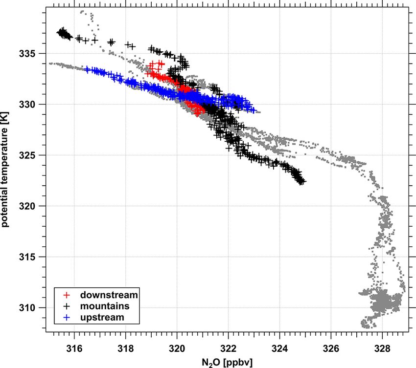
364                                                              H.-C. Lachnitt et al.: Gravity wave induced cross-isentropic mixing

Figure 7. Schematic evolution of potential temperature 2 versus N2 O in the presence of cross-isentropic mixing at the tropopause (e.g., by
orographic-wave-induced turbulence). The blue curve (a) shows the situation on the upstream side. The relation between N2 O and 2 (blue)
is modified by mixing (b; dotted black and shaded gray) over the mountains leading to a modified profile on the downstream side (c; red)
compared to the original upstream relation (blue). The dashed gray line shows the tropopause and the dashed light blue rectangle the flight
region of the upper leg.

                                                                            Figure 8 shows the measured N2 O profile as a function of
                                                                         potential temperature 2 for the entire flight FF09. The col-
                                                                         ored data points denote different longitudes relative to the
                                                                         mountain ridge to separate the inflow, across mountain, and
                                                                         downstream part of the flight leg (see Fig. 6). As evident from
                                                                         Fig. 8, different relations between 2 and N2 O appear on the
                                                                         upstream side, downstream side and above the mountains.
                                                                         The different relations are consistent with our hypothesis
                                                                         that the relationship between 2 and N2 O (and consequently
                                                                         the vertical gradient ∂N2 O/∂2) will be changed in regions
                                                                         impacted by gravity-wave-induced mixing. Upstream of the
                                                                         mountains this 2–N2 O relation shows a strong decrease of
                                                                         N2 O with increasing 2 and a compact relationship (i.e., a
                                                                         well-defined relationship exhibiting only weak scatter). On
                                                                         the downstream side, the N2 O decrease with respect to 2 is
                                                                         much weaker with intermediate values and larger variability
                                                                         above the mountains (see Fig. 8).

Figure 8. Profile of N2 O during FF09 (gray) as a function of poten-
tial temperature 2. The upper leg of the southwestern part is shown      4.1   Scale analysis
with different colors, indicating different flight sections along the
flight leg (blue: upstream, red: downstream, black: above the moun-      In a next step, we performed a scale-dependent correlation
tains, comp. Fig. 6).                                                    analysis as described below to further analyze the impact
                                                                         of the orographic waves on the 2–N2 O relation and to ac-
                                                                         count for a potential effect of different scales of the waves
the modified profile of N2 O compared to the upstream region             on cross-isentropic mixing. For this, we applied a Reynolds
(red versus blue slope).                                                 decomposition and separated the data into a mean part χ and
   Thus, in the case of gravity-wave-induced turbulent mix-              a perturbation part χ 0 (as well as 2 and 20 ):
ing during flight FF09, we expect a more rapid decrease
of N2 O with increasing 2 in the inflow region upwind the
                                                                         χ (t) = χ + χ 0 (t) ⇔ χ 0 (t) = χ(t) − χ .                    (4)
mountains than at the downstream side of the mountain ridge
as an effect of turbulent mixing. The vertical N2 O profile
with respect to 2 is modified from upstream to downstream                   The mean χ is calculated with a boxcar average which
due to turbulent mixing.                                                 works as a low-pass filter and removes high-frequency vari-
                                                                         ability. We analyzed the data for different averaging periods
                                                                         to account for varying perturbation wavelengths and at dif-

Atmos. Chem. Phys., 23, 355–373, 2023                                                       https://doi.org/10.5194/acp-23-355-2023
H.-C. Lachnitt et al.: Gravity wave induced cross-isentropic mixing 365
ferent scales using the following formula: the gravity waves over the mountain would occur. The ob-
Zt2 served peak-to-peak variability of 2 of 8 K (Fig. 6) would
1 correspond to N2 O = 13 ppbv, while only 4 ppbv are ob-
χ= χ(t)dt, (5)
t2 − t1 served consistent with an impact of diabatic mixing pro-
t1 cesses changing the upstream relation.
where t2 − t1 is the integration width. In summary, the ratio-changing behavior would be consis-
Above the tropopause, 2 increases while N2 O decreases. tent with a modification of the initial upstream N2 O profile
Thus, we expect an anti-correlation for the perturbations across the mountains, where the relation between 2 and N2 O
of these two quantities, 20 and N2 O0 , with a given slope is perturbed. When crossing the mountain ridge, gravity-
(or 20 /N2 O0 ratio) in the inflow region upstream of the wave-induced turbulence affects the 2–N2 O relation with
mountains. For linear non-dissipative waves, the 20 /N2 O0 a persistent effect at the downstream side. The downstream
ratio will therefore remain constant for different integration impact is evident from the different 20 /N2 O0 ratio at larger
widths. In the presence of non-conservative dissipative pro- wavelengths at the downwind side compared to the upstream
cesses, the linear relation between 20 and N2 O0 and thus their ratio. Therefore, we conclude that during FF09, mountain
ratio will change as explained above. waves modified the 20 /N2 O0 ratio by the generation of tur-
As an example, the effect of different integration intervals bulence at small scales. They induced cross-isentropic turbu-
on the distribution of data points is shown in Fig. 9 for two lent mixing leading to changes at large scales downwind of
different interval lengths. The applied fit accounts for errors the Alps as evident from the 20 /N2 O0 ratio and finally the
in x and y directions (Press et al., 1987). The figure shows the vertical gradient ∂N2 O/∂2 (Fig. 6).
same subset of data using averaging periods of 150 s (Fig. 9a) To identify the leading spatial and temporal scales for the
and 20 s (Fig. 9b) corresponding to a horizontal scale of 33 cross-isentropic (i.e., irreversible) mixing of N2 O, we ana-
and 4 km, respectively. For wavelengths shorter than these lyzed the wavelet coherence between the time series of N2 O
dimensions, the ratios at the downstream (red) and upstream and 2 in Fig. 11. Coherence is a measure of the intensity
(blue) side only slightly change. Both however clearly show of the covariance of 2 time series. At the upstream side
an increased ratio at the downstream side (red) compared to (< 170◦ E), there is mostly high coherence according to the
the upstream (blue). fact that 2 and N2 O co-vary across different timescales from
Above the mountains (black), the relation is perturbed, 1.7–17.3 km (corresponding to 8–80 s). Further, the phase re-
showing a high variability. The above-mountain ratio for lation between the time series of N2 O and 2 (see Fig. 6) is
the long waves (i.e., averaging periods, Fig. 9a) is closer to almost constant at 180◦ for scales < 20 km, which one would
the downstream side compared to the shorter wavelengths expect for opposing vertical gradients of N2 O and 2 in the
(Fig. 9b). stratosphere. Thus, both the wavelet coherence and the phase
To account for different scales and thus increasing wave- relation confirm the finding of the absence of mixing from
lengths, we subsequently increased the averaging period in the previous upwind slope analysis (Fig. 10, upstream side).
steps of 1 s from 2–292 s (length of the shortest data segment Above the mountains (from 170 to 171◦ E), there is low
unbroken by calibrations). The corresponding development coherence with values lower than 0.7 for timescales < 8,7 km
of the 20 /N2 O0 ratios is shown in Fig. 10. The blue curve is (< 40 s) accompanied by a breakdown of the phase relation
deduced from the data in the upstream region. With a value of between N2 O and 2, both indicating a decrease of the covari-
about −0.6 K ppbv−1 the ratio is almost constant over all av- ance. On the downstream side (from 171◦ E), especially at
eraging periods. This indicates that no cross-isentropic mix- small periods, higher coherence values and defined phase re-
ing perturbs the upstream linear 20 /N2 O0 ratio at any wave lations re-establish compared to the above-mountain regime,
period. albeit more variable than at the upstream side. Consistent
Indeed, in the long scale limit, a clear separation for the with Fig. 10, in upwind regimes with a high coherence, N2 O
downstream and above-mountain ratio is evident. The black and the potential temperature 2 co-vary: the phase relation
and red curves show a 20 /N2 O0 ratio change for differ- between them remains constant across scales and the calcu-
ent averaging periods. Above the mountains, the 20 /N2 O0 lated slope (Fig. 10) is unchanged too. Above the mountains,
ratio starts to change at longer averaging periods (100 s, the phase relation breaks down due to cross-isentropic mix-
21.6 km) compared to the downstream side. The changes at ing, especially for wave periods smaller than 6.5 km (30 s).
the downstream side start at shorter averaging periods (40 s, Downwind, a new ratio re-establishes as a result of mixing
8.7 km), indicating smaller scales or wavelengths relevant for above the mountain ridge, but with a defined phase relation
the change of the 20 /N2 O0 ratio. Downstream and above- again and different ratios.
mountain 20 /N2 O0 ratios merge for longer periods to the new We therefore conclude that above the mountains, the low
(modified) gradient with a 20 /N2 O0 ratio around 2 K ppbv−1 . coherence and the breakdown of the phase relationship at
Similar to Alexander and Pfister (1995), we used the up- short wavelength were an effect of the gravity waves which
stream relation between 2 and N2 O to estimate the N2 O am- produced turbulence and led to cross-isentropic mixing.
plitude which one would expect if only adiabatic transport by Therefore, the change in the 20 /N2 O0 ratio from the upwind
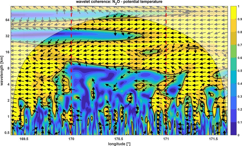
https://doi.org/10.5194/acp-23-355-2023 Atmos. Chem. Phys., 23, 355–373, 2023366 H.-C. Lachnitt et al.: Gravity wave induced cross-isentropic mixing
Figure 9. Relation between 20 and N2 O0 for upstream (blue), downstream region (red) and above mountains (black). (a) Averaging period of
150 s (32.5 km). (b) Averaging period of 20 s (4.3 km). The dotted lines indicate the slopes of the different flight segments. Note the changing
slope over the mountains.
The wavelet co-spectrum is calculated from the real part of
the cross-wavelet transformation and gives the spectral con-
tributions of vertical fluxes (Mauder et al., 2007). Figure 12
shows the co-spectrum of the cross-wavelet transformation
of N2 O and vertical wind w for the higher flight level during
FF09. There are two regions with enhanced fluxes within the
5 % significance level (solid black line), which are both lo-
cated above the mountains (compare Fig. 2). The first region
is between 170.0 and 170.6◦ E, the second between 170.8 and
171.0◦ E. The first region shows mainly positive trace gas
fluxes with values up to 0.50 ppbv m s−1 at wavelengths rang-
ing from 8–16 km, corresponding to the vertical wind energy
maximum around λx = 10 km Fig. 4. The second region ex-
Figure 10. Scale-dependent correlation anomaly analysis for dif- hibits upward and downward fluxes at slightly shorter scales
ferent integration times showing the 20 /N2 O0 ratio for different av- from about 3–16 km. Here, the strongest fluxes have values
eraging periods (i.e., wavelengths) for upstream (blue), downstream from about −0.22 to +0.56 ppbv m s−1 . The fluxes in both re-
(red) and above mountains (black). gions are co-located to enhanced wave occurrence above the
mountains, as seen in Figs. 6 and 2.
Since ozone was measured with a temporal resolution of
to the downwind side is the result of gravity-wave-induced 10 s, we did not directly determine ozone fluxes in the present
mixing. Since the mixing is cross-isentropic, this changed case. To give an estimate of the associated ozone flux, we can
the 20 /N2 O0 ratio, which is evident at the downstream side, use the N2 O–O3 correlation slope, which is about −20 ppbv
where a modified ratio establishes (compared to the upwind (O3 )/ppbv (N2 O) for the Southern Hemisphere in July (Heg-
side). glin and Shepherd, 2007). This results in a negative flux of O3
of 10 ppbv m s−1 for the positive N2 O-fluxes.
4.2 Fluxes
4.3 Turbulence occurrence
To estimate quantitative tracer fluxes, we use the co-spectrum
of the cross-wavelet transformation between the vertical The power spectral density (PSD) for 2 and the vertical wind
wind w and N2 O (see Sect. 2.4). Unlike other methods, the component w in Fig. 13 show a slope of −3 for wavelengths
wavelet analysis has the advantage to resolve wave-induced longer than 721 m (< 0.3 Hz), in agreement with the obser-
processes in space and time. vations of airborne measurements during START08 (2008
Atmos. Chem. Phys., 23, 355–373, 2023 https://doi.org/10.5194/acp-23-355-2023H.-C. Lachnitt et al.: Gravity wave induced cross-isentropic mixing 367 Figure 11. Wavelet coherence of N2 O and potential temperature (wavelength = period · flight speed (216 m s−1 ), see Eq. 2). Arrows to the left indicate that N2 O and potential temperature are shifted by 180◦ . In regions with a coherence lower than 0.5, the phase indication is removed. The shaded region marks the cone of influence, where edge effects affect the analysis. The solid lines show the 95 % confidence level as given in Sect. 2.4. Yellow colors indicate a high coherence and blue colors indicate a low coherence. Vertical lines mark the upstream, above mountain, and downstream side. Figure 12. (a) Co-spectrum of the cross-wavelet transformation of N2 O and vertical wind. The shaded region marks the cone of influence in which edge effects play a role. The black contour lines indicate 5 % significance levels against red noise. Red colors denote a positive flux and blue colors indicate a negative flux. (b) Scale-averaged wavelet co-spectrum over all periods. https://doi.org/10.5194/acp-23-355-2023 Atmos. Chem. Phys., 23, 355–373, 2023
368 H.-C. Lachnitt et al.: Gravity wave induced cross-isentropic mixing
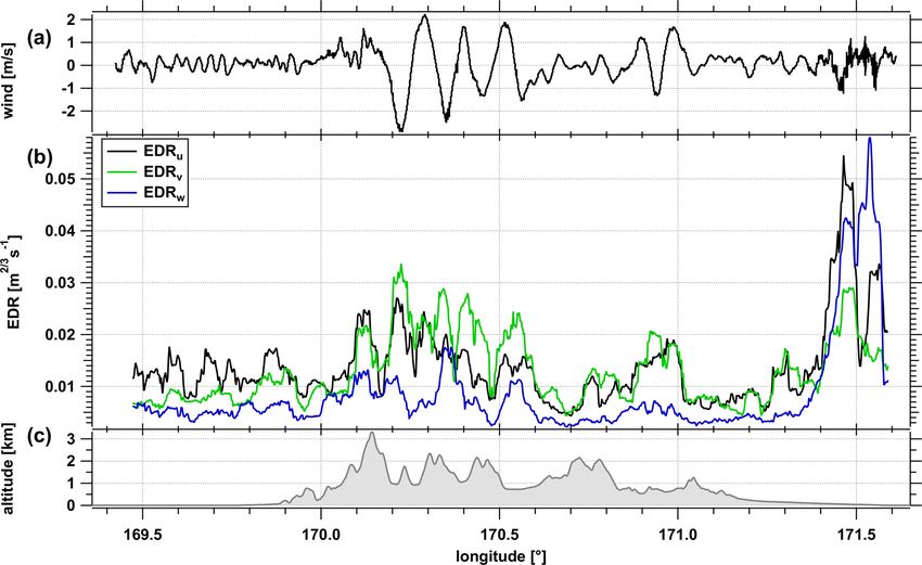
Further support for our hypothesis that mountain wave
induced turbulence perturbed the N2 O profile comes from
the analysis of the cube root of the eddy dissipation rate
EDR = 1/3 from the measured three-dimensional winds. For
this analysis, we used the method by Bramberger et al. (2018)
to calculate the EDR for the three wind components as mea-
sured by the aircraft (Fig. 14). Above the mountains, the os-
cillations of the vertical wind velocity w indicate the region
of mountain wave occurrence. The EDR over the mountains
appears to be weak below the threshold of light turbulence
of about 0.05 m2/3 s−1 (Bramberger et al., 2018). However,
the values of EDRu,v for the horizontal wind components are
enhanced over the mountain. In the lee of the mountains, the
EDR of all wind components is enhanced. Further support
for our hypothesis and our results comes from the analysis of
the occurrence of mountain-wave-induced turbulence using
the Graphical Turbulence Guidance (GTG) with ECMWF
operational analysis data (Bramberger et al., 2018; Sharman
et al., 2006; Sharman and Pearson, 2017). The GTG analysis
Figure 13. Power spectral density of vertical wind (blue), potential matches the observed locations of wave occurrence during
temperature (orange) and N2 O (black) for the flight segment above the flight and the regions of strong variability of the vertical
the mountains. The power spectral density has been smoothed by a
wind (not shown). Though the values are too high, this sup-
boxcar average of 5 s. The green and red reference lines have slopes
ports the conclusion that turbulence occurred in the region of
of −5/3 and −3.
the mixing events, either shortly before or during the mea-
surements.
The weak EDR at the upper flight leg in accordance with
Stratosphere–Troposphere Analyses of Regional Transport; the weak turbulence occurrence as opposed to the lower leg
Zhang et al., 2015) for wavelengths < 10 km. For shorter (see Fig. 4) may be explained by the time difference between
wavelengths (i.e., higher frequencies), the increase of the the two legs. As evident from the wave analysis, orographic
PSD at 433 m (0.5 Hz) would be consistent with a poten- waves were crossed during the first leg and led to wave break-
tial source of turbulent energy above the mountains. No- ing and momentum deposition in the region between the legs.
tably, a similar peak of the PSD of w was observed during At the higher leg, only a weak turbulence signal remained
the START08 campaign for some flight sections in regions 1 h later when the second crossing took place. The change of
of turbulence occurrence over the Rocky Mountains (Zhang ∂2/∂N2 O is a unique indication of a diabatic process, which
et al., 2015). However, the peak of the PSD from the verti- must have changed the gradient from the upstream to the
cal wind component around 433 m (0.5 Hz) could also cor- downwind side exactly above the mountains. The evidence
respond to oscillations caused by the autopilot of the air- for strong orographic wave activity at the lower level that
craft (Schumann, 2019). They report oscillations with wave- propagates to the 10.9 km level serves as the only plausible
lengths of 6.7 km in regions of high turbulence, which is a explanation for these observations. The fact that the turbu-
factor of 10 longer than in our case. Thus, an artificial non- lence is weak during the time of flight at the higher level
atmospheric origin of the peak cannot be completely ruled must be attributed to the time shift between the two flight
out. legs and the high intermittency of turbulence.
For wavelengths below 108 m (> 2 Hz), the slope of the
PSD of both w and 2 approach −5/3, which can be re-
lated to isotropic turbulence. Figure 13 also shows the PSD 5 Conclusions
of N2 O. It has a slope of −3 for longer wavelengths (smaller
frequencies) and a flattening slope for wavelengths smaller We present an analysis of high-resolution N2 O measure-
than 721 m (> 0.3 Hz). A change of the turbulent behavior as ments in the region of orographic gravity waves over the
indicated by the transition of PSD slopes occurs in the wave- Southern Alps in New Zealand during the DEEPWAVE 2014
length range between 271 to 721 m (corresponding to 0.8 campaign. These gravity waves led to diabatic trace gas
to 0.3 Hz), where the PSD of the vertical wind indicates a fluxes and a persistent local effect on the composition down-
source of turbulent energy. Notably, the PSD of N2 O points wind of the mountain and the above the tropopause.
to a turbulent behavior for small wavelengths and thus the The spectral analysis of the wind components measured
occurrence of turbulent fluxes corresponding to the analysis along two vertically stacked levels indicates dissipation of
in the previous section. momentum by orographic waves above the mountains be-
Atmos. Chem. Phys., 23, 355–373, 2023 https://doi.org/10.5194/acp-23-355-2023H.-C. Lachnitt et al.: Gravity wave induced cross-isentropic mixing 369 Figure 14. Time series of (a) vertical wind, (b) EDR for the measured wind components for the upper flight leg indicating weak, but non-vanishing turbulence during the time of flight above the Southern Alps (orography shown in c). tween these levels and the generation of turbulence. The leg explains why the turbulent kinetic energy for w0 at short spectral energy of the vertical wind component shows strong horizontal wavelengths is rather small compared to the lower signals at short horizontal wavelengths (< 1 km) at the lower leg. Still, the power spectral energy spectra of N2 O and 2 flight leg at 7.9 km. At the higher leg, which was flown with slopes of −5/3 at the smallest scales can be seen as the 75 min later in the stratosphere, horizontal wavelengths of result of the turbulence that may have occurred on this level. 10 km dominate the energy spectrum of w 0 with much The tracer distribution conserves the effect of prior oc- weaker contribution at the shorter scale. Corresponding to currence of highly transient turbulence occurrence. At the the fluctuations of the vertical wind and potential tempera- downstream side, a modified compact N2 O–2 relation es- ture 2, strong fluctuations of the tracer N2 O were also ob- tablishes as a result of the wave-induced turbulence above the served at the upper flight leg in the region of the occurrence mountains. The reversible air mass displacements induced by of orographic waves. Based on the analysis of the CO–N2 O the gravity waves are similar to the mechanism described in relationship, we could identify mixing between two layers of (Moustaoui et al., 2010; Mahalov et al., 2011). This behavior different air masses in the tropopause region. Upstream and is confirmed by cross-wavelet analyses showing a breakdown downstream of the mountain, different vertical gradients of of the coherence and phase relationship between N2 O and 2 N2 O with respect to potential temperature 2 were observed over the mountains. and enhanced variability of this gradient was observed above The vertical fluxes of N2 O are estimated to be the mountains. Since N2 O is chemically inert, a change of 0.5 ppbv m s−1 , corresponding to negative fluxes of O3 of ap- the N2 O–2 relation must be due to cross-isentropic mixing proximately 10 ppbv m s−1 . effects. The change of the 2–N2 O relation from the upstream to A scale-dependent slope analysis shows that mixing was the downstream side over the mountain ridge is a unique in- initiated over the mountain ridge with reversible displace- dicator for cross-isentropic (i.e., irreversible) turbulent ex- ments of tracer isopleths and 2. These fluctuations must change of species, which was initiated by the orographic have perturbed the compact relation between 2 and N2 O via waves. The fact that the modified relationship prevails down- the generation of turbulence and thus irreversible turbulent stream of the mountain shows that the turbulence associ- cross-isentropic mixing. ated with the orographic waves was associated with cross- Mountain-wave-induced mixing is also consistent with isentropic mixing. The approach using the 2–N2 O relation the indication for wave breaking and momentum deposition notably differs from local covariance analysis of vertical above the mountains between the two flight legs. Noting that winds and tracers since it shows that at least part of the kine- the stratospheric flight leg was flown 75 min after the lower matic fluxes contributed to a cross-isentropic component. https://doi.org/10.5194/acp-23-355-2023 Atmos. Chem. Phys., 23, 355–373, 2023
You can also read