Implementation of aerosol data assimilation in WRFDA (v4.0.3) for WRF-Chem (v3.9.1) using the RACM/MADE-VBS scheme
←
→
Page content transcription
If your browser does not render page correctly, please read the page content below

Geosci. Model Dev., 15, 1769–1788, 2022
https://doi.org/10.5194/gmd-15-1769-2022
© Author(s) 2022. This work is distributed under
the Creative Commons Attribution 4.0 License.

Implementation of aerosol data assimilation in WRFDA (v4.0.3) for
WRF-Chem (v3.9.1) using the RACM/MADE-VBS scheme
Soyoung Ha
National Center for Atmospheric Research, Boulder, CO, USA

Correspondence: Soyoung Ha (syha@ucar.edu)

Received: 11 March 2021 – Discussion started: 2 June 2021
Revised: 13 October 2021 – Accepted: 18 January 2022 – Published: 2 March 2022

Abstract. The Weather Research and Forecasting model              with long-range transport of pollutants, so the changes in lo-
data assimilation (WRFDA) system, initially designed for          cal emissions in the upstream areas can affect the chemical
meteorological data assimilation, is extended for aerosol         composition and the PM concentrations in the region to a
data assimilation for the WRF model coupled with chem-            great extent (Jo et al., 2020). Given the considerable effect
istry (WRF-Chem). An interface between WRF-Chem and               of meteorological simulations on the chemical processes and
WRFDA is built for the Regional Atmospheric Chemistry             the large uncertainty in the chemical transport models, chem-
Mechanism (RACM) chemistry and the Modal Aerosol Dy-              ical (or aerosol) data assimilation in the numerical weather
namics Model for Europe (MADE) coupled with the Volatil-          prediction (NWP) system coupled with chemistry can make
ity Basis Set (VBS) aerosol schemes. This article describes       encouraging contributions to short-range air quality forecast-
the implementation of the new interface for assimilating          ing, with better representation of the atmospheric composi-
PM2.5 and PM10 as well as four gas species (SO2 , NO2 , O3 ,      tion at the initial time.
and CO) on the ground. The effects of aerosol data assimi-           The Weather Research and Forecasting model’s commu-
lation are briefly examined through a month-long case study       nity data assimilation system (WRFDA; Barker et al., 2012)
during the Korea–United States Air Quality (KORUS-AQ)             developed by the National Center for Atmospheric Research
period. It is demonstrated that the improved chemical ini-        (NCAR) was initially designed for meteorological data as-
tial conditions through the 3D-Var analysis can lead to con-      similation to initialize the WRF model (Skamarock et al.,
sistent forecast improvements up to 26 %, reducing system-        2008) using a variational or a hybrid data assimilation tech-
atic bias errors in surface PM2.5 (PM10 ) concentrations to 0.0   nique. Since the NWP model was coupled with chemistry
(−1.9) µg m−3 over South Korea for 24 h.                          and aerosol dynamics as an integrated forecasting system
                                                                  (WRF-Chem; Grell et al., 2005), it has been widely used for
                                                                  regional air quality forecasting, representing two-way real-
                                                                  time interactions between meteorology and chemistry (Grell
1   Introduction                                                  and Baklanov, 2011), but WRFDA has remained for use in
                                                                  weather data assimilation until very recently.
Regional air quality forecasting is mainly concerned with            Unlike meteorological data assimilation, where most prog-
air pollutants confined to the boundary layer (up to 1 km         nostic variables (except hydrometeors) remain the same re-
from the ground), which is predominantly characterized by         gardless of the physics schemes in use, aerosol data assimi-
near-surface concentrations of particulate matter (PM) with       lation is tied to the chemistry parameterization employed in
particle diameters less than 2.5 and 10 µm (e.g., PM2.5 and       the chemical transport model. That is because each chemical
PM10 , respectively). Many processes, such as the transport       option (for both gas and aerosol chemistry) defines an en-
and dispersion of chemical species, that directly affect sur-     tirely different set of chemical and aerosol prognostic vari-
face concentrations, strongly depend on weather conditions        ables. It implies that PM concentrations consist of different
(Baklanov et al., 2017). In particular, frequent haze events      aerosol species, depending on the chemical option used in the
with high PM concentrations over Korea are often associated

Published by Copernicus Publications on behalf of the European Geosciences Union.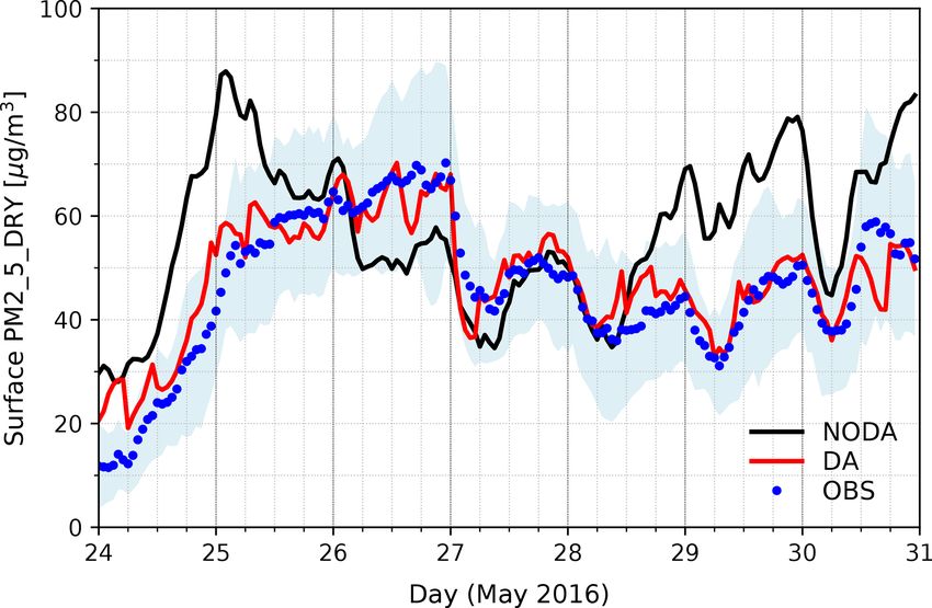
1770                                                S. Ha: Aerosol data assimilation using the RACM/MADE-VBS scheme

WRF-Chem model. Therefore, to assimilate PM measure-              WRF-Chem model. This chemical option is expected to pro-
ments, a new interface has to be developed in WRFDA for the       vide a more realistic representation of organic carbon, nitrate,
particular chemistry option (chem_opt), containing new ob-        and SOA that often resulted in the PM2.5 underestimation
servation operators (that compute the model correspondents        over the East Asian region (Lee et al., 2020; Jo et al., 2020).
from the specific aerosol species), their tangent linear and         The main goal of the new system development is to facili-
adjoint models as well as the background error covariance         tate aerosol data assimilation using the RACM/MADE-VBS
estimation. In other words, even if the WRF-Chem model            scheme (chem_opt = 108) in the WRF-Chem/WRFDA sys-
supports numerous chemical parameterization options, they         tem so that the initial conditions can lead to better air qual-
cannot be used interchangeably in the WRFDA system be-            ity forecasting, especially in surface PM2.5 concentrations
cause the analysis variables are tied to the aerosol species      over Korea. This study introduces the new system and ex-
defined in the chemistry scheme. In practice, users should        amines how the assimilation of surface observations can af-
use the same chemical option between the forecast model           fect air quality forecasts through month-long cycling exper-
and the analysis system, meaning that the particular chemi-       iments for May 2016, the Korea–United States Air Quality
cal option should be implemented in the assimilation system       (KORUS-AQ) campaign period. During early summertime,
in advance. That is why chemical or aerosol data assimila-        air quality was measured in various platforms over the Ko-
tion studies have used a minimal set of chemical options so       rean Peninsula and its surroundings, and long-range transport
far and why it is challenging to use advanced chemistry in        of air pollutants resulted in haze development over Korea for
aerosol data assimilation studies within the variational anal-    25–31 May 2016. For the details of the case or the field cam-
ysis framework.                                                   paign, readers are referred to several other papers (Ha et al.,
   Other challenges for chemical data assimilation are large      2020, Peterson et al., 2019, and Miyazaki et al., 2019).
model uncertainties due to the complexity of chemical pro-           An overview of the new WRF-Chem/WRFDA system, in-
cesses, significant uncertainties in forcing parameters such      cluding new forward operators and background error statis-
as emissions, highly nonlinear and non-Gaussian error dis-        tics, is presented in Sect. 2, followed by cycling experiments
tribution of chemical species, and expensive computations         and the forecast verification against independent observa-
ascribed to a long list of chemical species – typically with      tions described in Sect. 3. Finally, conclusions are made in
dozens or hundreds of prognostic variables. The latter makes      Sect. 4, followed by a discussion on the limitations of this
the three-dimensional variational data assimilation (3D-Var)      study and suggestions for future research.
algorithm still attractive, especially in the operational envi-
ronment, even with its limitations such as static background
error covariance and the use of the linearized forecast model     2   The WRF-Chem analysis and forecasting system
during the minimization procedure.
   Because of the simplicity and the effective cost, the bulk     The WRF-Chem model has many options for gas and aerosol
Goddard Chemistry Aerosol Radiation and Transport (GO-            chemistry parameterizations that are fully coupled with me-
CART; Chin et al., 2002) aerosol scheme has long been used        teorology, facilitating aerosol direct and indirect effects
for aerosol data assimilation (Liu et al., 2011, Saide et al.,    through interactions with radiation, photolysis, and micro-
2014, and Ha et al., 2020, just to name a few), although it is    physical processes in real time (Fast et al., 2006). Within the
well known to underestimate ground PM concentrations due          WRF infrastructure, it is coupled with the WRF preprocess-
to the lack of secondary organic aerosol (SOA) formulation        ing system (WPS) and data assimilation (WRFDA), so it can
(McKeen et al., 2009, Hallquist et al., 2009).                    fully support the analysis and forecasting with the coupled
   To use a more sophisticated chemistry option in aerosol        evolution of weather and chemistry. As the processes like ad-
data assimilation, Sun et al. (2020) recently implemented         vection and diffusion are applied for both chemical and mete-
a new interface between WRF-Chem and WRFDA for the                orological variables, chemical species are transported based
Carbon Bond Mechanism version Z (CBMZ; Zaveri and Pe-             on the model time step (which depends on the grid resolu-
ters, 1999) gas chemistry and Model for Simulating Aerosol        tion).
Interactions and Chemistry (MOSAIC; Zaveri et al., 2008)             Data assimilation pulls model trajectories toward the ob-
aerosol schemes. They assimilated surface measurements us-        served information at the initial time, but when the model
ing the 3D-Var technique and demonstrated systematic im-          integration starts from the initial state, the forecast model
provements of air quality forecasting over China up to 24 h.      tries to restore its own climatology based on the assumptions
   This study extends the WRF-Chem/WRFDA 3D-Var sys-              and parameters defined in the system. Hence, to prevent the
tem for the Regional Atmospheric Chemistry Mechanism              model state from drifting away from the observed state, the
(RACM; Stockwell et al., 1997) gas-phase chemistry, cou-          analysis (or data assimilation) should be conducted repeat-
pled with the Modal Aerosol Dynamics Model for Europe             edly, incorporating various observations into the model and
(MADE; Ackermann et al., 1998) and the secondary organic          updating initial conditions at certain time intervals (e.g., ev-
aerosol (SOA) scheme based on a four-bin Volatility Basis         ery 6 h). By conducting the analysis and the forecast con-
Set (VBS) (Ahmadov et al., 2012) in version 3.9.1 of the          secutively (so-called “cycling”), initial conditions and subse-

Geosci. Model Dev., 15, 1769–1788, 2022                                           https://doi.org/10.5194/gmd-15-1769-2022
S. Ha: Aerosol data assimilation using the RACM/MADE-VBS scheme                                                             1771

quent forecasts can be systematically improved in the long
term. For such a unified, synthetic cycling system, the anal-
ysis and the forecast systems communicate through an inter-
face that converts between observed variables, analysis (or
control) variables, and model prognostic variables.
   By default, chemical boundaries are reset based on the ide-
alized profiles specified in the chemistry routines in WRF-
Chem. But if the chemical lateral boundary option (e.g.,
“have_bcs_chem”) is turned on to provide more realistic in-
flows of chemicals, wrfbdy files also need to be updated
for chemical species, typically using the output from global
chemical forecasts.
   Unlike the cycling for weather forecasting, chemical sim-
ulations typically recycle chemical variables from the pre-
vious forecasts, which are provided through an auxiliary in-
put stream (e.g., wrf_chem_input) for the initialization (with
real.exe). At this time, WRF-Chem also needs several ad-
ditional input files for various emissions data because the
chemical transport model is strongly driven by the forcing         Figure 1. The surface observation network in two model domains.
parameters throughout the model integration and heavily re-        A black box indicates domain 2 (D2) over South Korea, nested
lies on the quality of the emissions data produced for the         down from domain 1 (D1). Colored dots indicate surface PM2.5
region. Once the initial conditions (e.g., wrfinput files) are     observations assimilated on 26 May 2016 at 00:00:00 UTC.
produced by the initialization, they are used as background
(e.g., a priori) for the analysis update at the cycle. (If data
assimilation is not carried out, the initial conditions are not    from the 20-class, 30 arcsec MODIS data through the geogrid
updated any further and directly used to initialize the model      program of the WRF preprocessing system (WPS). The ini-
simulation with the chemistry fields predicted from the pre-       tial and lateral boundary conditions for meteorological vari-
vious cycle.) In the presented work, chemical observations         ables are produced by global forecasts from the UK Met Of-
are assimilated along with in situ meteorological measure-         fice’s Unified Model (UM) operated by the Korean Meteo-
ments. But even if weather data are not assimilated, mete-         rological Administration (KMA) every 6 h. For meteorolog-
orological fields are updated through initial and boundary         ical data assimilation, conventional observations in the Na-
conditions and the online interactions between aerosol and         tional Centers for Environmental Prediction (NCEP) prep-
radiation during the forecast step. Once the assimilation is       bufr data (https://rda.ucar.edu/datasets/ds337.0/; last access:
done, wrfbdy files are updated in the mother domain before         4 March 2021) are employed.
the model prediction starts in order to become consistent with        This study focuses on the RACM gas chemistry
the analysis fields in the relaxation zone. But such boundary      and the MADE-VBS aerosol parameterization (e.g.,
updates are not applied to the chemical fields because chem-       chem_opt = 108) in WRF version 3.9.1. The MADE-VBS
ical or aerosol observations within five grids (51x) from the      aerosol scheme defines a superposition of three log-normal
boundary cells are not assimilated (e.g., no analysis updates      modes – Aitken, accumulation, and coarse modes – based on
near the lateral boundaries).                                      the particle size distribution: an Aitken mode with a median
                                                                   diameter of 0.01 µm, an accumulation mode ranging between
2.1   The WRF-Chem configuration                                   0.01 and 1 µm, and a coarse mode for particles typically
                                                                   larger than 1 µm (with a median around 10 µm). All aerosol
The model simulations cover the East Asian region and the          particles are assumed to be spherical and internally mixed
Korean Peninsula with 27 and 9 km grid resolution, respec-         (Aquila et al., 2011). The aerosol species treated are sulfate
                                                                                        +                   +
tively, in a one-way nesting mode, as shown in Fig. 1. Verti-      (SO= 4 ), nitrate (NO3 ), ammonium (NH4 ), elemental carbon
cally, 31 model levels are configured up to 50 hPa, with the       (EC), primary organic matter (POA), anthropogenic and
lowest level located around 173 m in domain 2. Such a coarse       biogenic secondary organic aerosol (SOA), chloride (Cl),
vertical resolution may not resolve the observed spatial and       sodium (Na), unspeciated PM2.5 , unspeciated coarse fraction
temporal variability of atmospheric aerosols, but the config-      of PM10 (antha), soil dust, and sea salt. The unspeciated
uration is adopted from the current operational setting in the     PM2.5 includes the fine fraction of sea salt and mineral dust
National Institute of Environment Research (NIER) in South         aerosols.
Korea.                                                                The dust and sea salt emissions are simulated fol-
   Static geographical fields such as land use, vegetation frac-   lowing the GOCART mechanism (e.g., dust_opt = 13 and
tion, albedo, soil temperature, and soil moisture are obtained     seas_opt = 2). Photolysis rates of chemical species are com-

https://doi.org/10.5194/gmd-15-1769-2022                                             Geosci. Model Dev., 15, 1769–1788, 2022
1772                                                   S. Ha: Aerosol data assimilation using the RACM/MADE-VBS scheme

Table 1. Summary of WRF-Chem physics configuration.

                                 Physical processes      Parameterization schemes
                                 Aerosol chemistry       RACM (Stockwell et al., 1997)
                                 Gas-phase chemistry     MADE-VBS (Ackermann et al., 1998)
                                 Photolysis              Madronich (Madronich, 1987)
                                 Cloud microphysics      Lin (Chen and Sun, 2002)
                                 Cumulus                 Grell 3D ensemble (Grell and Dévényi, 2002)
                                 Longwave radiation      RRTMG (Iacono et al., 2008)
                                 Shortwave radiation     RRTMG (Iacono et al., 2008)
                                 PBL                     YSU (Hong et al., 2006)
                                 Surface layer           Monin–Obukhov (Jimenez et al., 2012)
                                 Land surface            Noah (Chen and Dudhia, 2001)

puted in a simplified version of the National Center for             conditions for domain 1, chemical species in CAM-Chem
Atmospheric Research (NCAR) tropospheric ultraviolet–                are converted to the RACM gas species in WRF-Chem
visible (TUV) model (named the Madronich scheme)                     through the “mozbc” utility (https://www2.acom.ucar.edu/
(Madronich, 1987), and the Rapid Radiative Transfer                  wrf-chem/wrf-chem-tools-community/, last access: 28 De-
Model for GCMs (RRTMG) is used for both shortwave                    cember 2020).
(ra_sw_physics = 4) and longwave (ra_lw_physics = 4) ra-
diation (Iacono et al., 2008). The direct aerosol effect is ac-      2.2   WRFDA for WRF-Chem
counted for through interactions with atmospheric radiation
and photolysis. A list of physics and chemistry schemes used         A new interface for the RACM/MADE-VBS scheme is de-
in this study is summarized in Table 1.                              veloped based on version 4.0.3 of the WRFDA system to
   Anthropogenic emission data are obtained from the KO-             assimilate PM2.5 , PM10 , SO2 , NO2 , O3 , and CO measure-
RUS version 2 inventory, originally developed based on the           ments on the ground. The variational data assimilation sys-
Comprehensive Regional Emissions for Atmospheric Trans-              tem seeks an analysis solution as the best estimate of the
port Experiment (CREATE-2015) emissions dataset and up-              true state by minimizing deviations of model variables (x)
dated for the KORUS-AQ campaign (Woo et al., 2012; Choi              from the corresponding observations (y) based on the error
et al., 2019). They were all emitted at the surface, i.e., with-     statistics of background forecasts and observations. The vari-
out any plume rise or specified vertical distribution. Note          ational scheme assumes Gaussian and unbiased error distri-
that anthropogenic emission data should be produced for the          butions, which can be characterized by covariances alone; its
chemistry variables defined in the chemical option. Biogenic         solution is thus found a least-squares best fit using the covari-
emissions are built up online using the Model of Emission of         ances. In practice, when the cost function J (x) is reached to
Gases and Aerosol from Nature (MEGAN; Version 2) (Guen-              a minimum through an iterative minimization process, the re-
ther et al., 2006), but biomass burning emissions are not used       sulting state vector x becomes the analysis solution (Lorenc,
in this study. All the WRF files including anthropogenic and         1986).
biogenic emissions are processed based on the MODIS land-                               1
use datasets (Friedl et al., 2002).                                  J (x) = J b + J o = (x − x b )T B−1 (x − x b )
                                                                                        2
   For chemical lateral boundary conditions, 6-hourly global
                                                                                          1
outputs from the Community Atmosphere Model with                                        + (y − H (x))T R−1 (y − H (x)),           (1)
Chemistry (CAM-Chem) model, a component of the Com-                                       2
munity Earth System Model (CESM) version 2.1, were                   where x b is the background state vector, which is usually
used (Buchholz et al., 2019). These simulations were con-            obtained from a deterministic forecast from the previous as-
figured at 0.9◦ × 1.25◦ horizontal resolution and 56 ver-            similation cycle, and B and R represent background and ob-
tical levels up to 1.9 hPa using an updated tropospheric             servation error covariance matrices, respectively. An obser-
chemistry mechanism (MOZART-T1; Emmons et al., 2020),                vation operator H (x) transforms the model states (x) to the
the Modal Aerosol Model with four modes (MAM4;                       observed quantities (y) at observation locations and can be
Liu et al., 2016), the anthropogenic and biomass burn-               nonlinear.
ing emissions from the inventories specified for Climate                The WRFDA employs an incremental formulation
Model Intercomparison Project 6 (CMIP6), and meteorolog-             (Courtier et al., 1994) where the model state vector (x) is
ical fields specified from Modern-Era Retrospective anal-            replaced by increments δx(= x − x b ) and the minimization
ysis for Research and Applications (MERRA)-2 reanal-                 algorithm is constructed as a pair of nested loops. The full,
ysis (Molod et al., 2015). To make chemical boundary                 nonlinear model is used at each iteration of the outer loop,

Geosci. Model Dev., 15, 1769–1788, 2022                                               https://doi.org/10.5194/gmd-15-1769-2022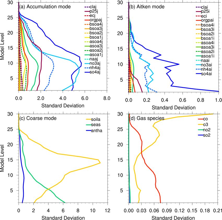
S. Ha: Aerosol data assimilation using the RACM/MADE-VBS scheme                                                               1773

while its linearized version – tangent linear and adjoint mod-     bsoa4j) with i and j at the end of each variable name in-
els – is used in the inner loop to adjust the model trajectory     dicating Aitken and accumulation modes, respectively. Also
and minimize J iteratively. This approach can keep analysis        included are three coarse-mode variables – non-reactive an-
imbalance to a minimum, making the minimization proce-             thropogenic aerosol (antha), marine aerosol concentration
dure more efficient. The final analysis x a (= x b + δx) is then   (seas), and soil-derived aerosol particles such as dust (soila) –
used as the initial condition for the model simulation.            and four gas species (SO2 , NO2 , O3 , and CO).
   In most NWP models, the state vector (x) that contains             The WRFDA provides various options for estimating the
all the prognostic variables lies in the huge dimensional state    background error covariance through “cv_option” in the
space (with typical degrees of freedom greater than O(107 )),      namelist. Here, cv_option = 7 is chosen for no balance trans-
which makes the computation of the inverse matrix (B−1 )           formation in the regional simulations, meaning that the
prohibitive. As a practical way of solving J b , a control vec-    chemical and aerosol species are control variables as full
tor (v) that consists of analysis variables is defined as δx =     fields and no cross correlations are considered between the
B1/2 v. While forecast errors of model variables are typically     variables such that Up becomes an identity operator. The hor-
correlated through governing equations, control variables are      izontal transform matrix Uh is performed using recursive fil-
designed to have no cross correlations such that the error ma-     ters (Purser et al., 2003), while the vertical transform Uv is
trix is diagonalized. With the control variable transformation,    carried out via an empirical orthogonal function (EOF) de-
the cost function is rewritten as below.                           composition of the vertical component of the background er-
                                                                   ror covariance.
       1       1
J (v) = v T v + (d − HB1/2 v)T R−1 (d − HB1/2 v),           (2)       In the 3D-Var algorithm, the estimation of background er-
       2       2                                                   ror covariance is critical, especially in data-sparse regions.
where the innovation vector is defined as d = y − H(x b ) and      As most surface stations are concentrated in urban areas, the
H is a linearized version of H . The square root of the B ma-      structure of background error covariance determines how to
trix (B = B1/2 (B1/2 )T ) is decomposed into a series of sub-      spread out the observed information horizontally and verti-
matrices for the control variable transform so that the cost       cally. In aerosol data assimilation, it is of particular impor-
function can avoid the inverse calculation of the large B ma-      tance as the atmospheric constituents are adjusted according
trix.                                                              to their background errors (e.g., B1/2 in δx = B1/2 v).
                                                                      In this study, chemical simulations are carried out in the
B1/2 = Up SUv Uh ,                                          (3)    WRF-Chem model, starting at 00:00 UTC every day for one
                                                                   month in May 2016, to compute background error covari-
where the Up matrix is called physical or balance transfor-        ance statistics for chemical and aerosol species defined in the
mation (via linear regression), S a diagonal matrix of fore-       RACM/MADE-VBS parameterization. Differences between
cast error standard deviation, Uv the vertical transform, and      24 and 48 h forecasts at the same validation time are then
Uh the horizontal transform matrix.                                used as a proxy for forecast errors in each domain, and a
   In weather data assimilation, the control variable trans-       total of 29 sample forecasts for 3–31 May 2016 were used
formation has been broadly practiced because meteorolog-           to construct the B matrix using the National Meteorological
ical variables follow physical balance equations (such as          Center (NMC) method (Parrish and Derber, 1992), assuming
geostrophic or hydrostatic equations) at large scales (Bannis-     the same model bias and uncorrelated model errors. There
ter, 2008). But it is not straightforward to define multivariate   are five sequential stages (e.g., stage0–stage4) implemented
correlations between chemical species or between chemical          with different options in the GENBE software. In this study,
and meteorological variables due to their complex interac-         all the grid points are binned together for each model level,
tions and chemical reactions that are highly nonlinear and         with no latitudinal or longitudinal dependencies in the back-
often transient. Therefore, chemical or aerosol species in the     ground error covariance.
model states (x) are directly used as control variables (v)           Figure 2 displays the vertical profile of the background er-
with univariate error covariances in chemical data assimila-       ror standard deviation of each species over domain 2. During
tion.                                                              the analysis procedure, the error is used to weigh the analysis
   To compute the background error covariance matrix (B)           increment for a given variable, affecting how much the ob-
for atmospheric constituents defined in the RACM/MADE-             served information will change the model variable. Depend-
VBS scheme, the GEN_BE v2.0 (Descombes et al., 2015)               ing on the aerosol size distribution, Aitken-, accumulation-
software is expanded for 39 three-dimensional chemical vari-       , and coarse-mode variables are compared separately. Most
ables: aerosol sulfate (so4ai and so4aj), nitrate (no3ai and       aerosol species in the accumulation mode have relatively
no3aj), ammonium (nh4ai and nh4aj), chloride (clai and             large background error standard deviations in the boundary
claj), primary organic matter (orgpai and orgpaj), elemen-         layer, and their counterparts in the Aitken mode show 1 or-
tal carbon (eci and ecj), sodium (naai and naaj), unspeci-         der magnitude smaller values, mostly with the maximum at
ated PM2.5 (p25ai and p25aj), four-bin anthropogenic and           the surface. Among the species, large background errors are
biogenic SOA (asoa1i, asoa1j, asoa2i, asoa2j, . . . , bsoa4i,      found in sulfate, nitrate, ammonium, and unspecified PM2.5 ,

https://doi.org/10.5194/gmd-15-1769-2022                                             Geosci. Model Dev., 15, 1769–1788, 2022
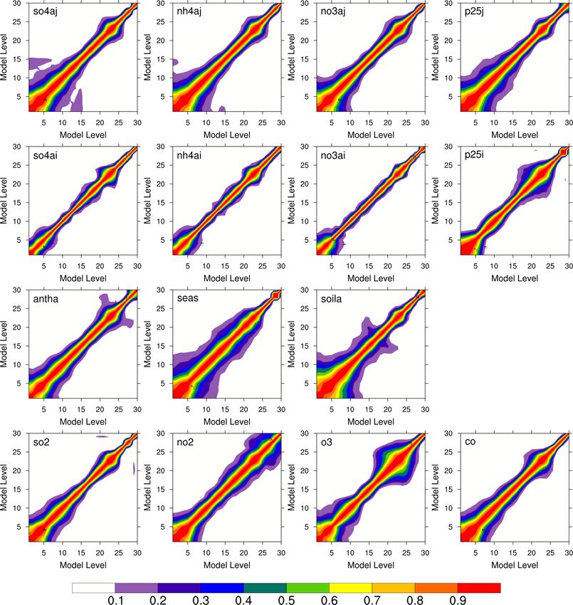
1774                                                    S. Ha: Aerosol data assimilation using the RACM/MADE-VBS scheme

Figure 2. Vertical profile of background error standard deviations for aerosol species in (a) accumulation, (b) Aitken, and (c) coarse modes,
and (d) gas species over domain 2.

contributing most to PM2.5 concentrations. In the coarse                 accumulation- and coarse-mode particles have a wider ver-
mode, sea salt linearly reduces with height, indicating large            tical spread than the Aitken-mode particles with more lo-
contributions (to PM10 ) at the sea level, but soila is charac-          calized effects. The round pattern around level 22 in most
terized by the high peak in the mid-troposphere, which might             species could be related to the advection with strong upper-
be associated with the long-range transport of dust aerosols.            level jets. While all the trace gases have relatively large cor-
In the gas species, ozone (O3 ) represents large errors near the         relations near the surface, ozone and nitrogen dioxide show
top (e.g., low stratosphere), while carbon monoxide (CO) is              the largest correlations near the tropopause and stratosphere,
concentrated in the low troposphere. Due to the trivial val-             respectively.
ues, the vertical error structures of SO2 and NO2 are hard to               To examine the horizontal propagation of the increments
see, but their standard deviations are also relatively large in          from point observations, the horizontal correlation length
the boundary layer.                                                      scales of the same species are illustrated in Fig. 4. In accu-
   The vertical spread of the observed information at the sur-           mulation and coarse modes (in the top and the third rows,
face is determined by vertical error correlations, closely as-           respectively), the overall vertical structure is similar, with
sociated with the simulated boundary layer height. As the                the linear increase down to the surface. The length scale at
static background error covariance cannot simulate the diur-             the surface is specified around 36 km for so4aj, for example,
nal variability of the boundary layer, this becomes one of the           corresponding to four grids in the 9 km domain, meaning that
main limitations of the 3D-Var analysis for air quality appli-           an observation at a point location can affect four surrounding
cations. Figure 3 depicts the normalized vertical autocorre-             grid points radially. On the other hand, Aitken-mode aerosols
lations derived from the time-lagged forecasts for four ma-              have short length scales near the surface, which tend to in-
jor aerosol species in accumulation and Aitken modes, three              crease in the upper levels, but their maximum values are
coarse-mode aerosols, and four trace gases (from top to bot-             smaller than those of their counterparts in the accumulation
tom panels). Generally, correlation contours tend to spread              mode, representing more localized effects horizontally. Trace
more in the lower levels, implying that the analysis updates             gases show different vertical distributions with the maximum
in the lowest level can affect the entire boundary layer. The            near the top, except for ozone.

Geosci. Model Dev., 15, 1769–1788, 2022                                                    https://doi.org/10.5194/gmd-15-1769-2022

S. Ha: Aerosol data assimilation using the RACM/MADE-VBS scheme                                                                     1775

Figure 3. Vertical autocorrelations in four major aerosol species in accumulation and Aitken modes (in the first and second rows, respec-
tively), three coarse-mode aerosols (in the third row), and four gas species (in the bottom row) over domain 2, contouring from 0.1 to 0.9
every 0.1 in different colors.

   When     the    RACM/MADE-VBS           option     (e.g.,           (µg m−3 ), and N = 16. To be consistent with the way the
chem_opt = 108) is chosen, the model equivalent of                     MADE-VBS aerosol scheme estimates PM2.5 concentrations
the observed PM2.5 (XPM2.5 ) is computed as a total sum of             in the model, the observation operator in WRFDA uses the
three-dimensional mass mixing ratios of 32 aerosol species             same equation as in Eq. (4), having individual species in dif-
in accumulation (j ) and Aitken (i) modes predicted in the             ferent modes contributing to the PM concentrations equally.
WRF-Chem model, as below.                                              If the observed atmospheric composition significantly differs
                j
              N X                                                      from the one in the model, or particular species change pre-
                         p                                             dominantly at certain times, this approach can lead to erro-
              X
XPM2.5 = ρd             xm,                                    (4)
              p=1 m=i                                                  neous results (in both the analysis and forecast).
                                                                          When PM10 is assimilated alone, the model correspon-
where ρd is dry density ([kg m−3 ]) for the unit conversion            dent is computed by adding three coarse-mode variables –
from aerosol mixing ratios (µg kg−1 ) to mass concentrations

https://doi.org/10.5194/gmd-15-1769-2022                                                   Geosci. Model Dev., 15, 1769–1788, 2022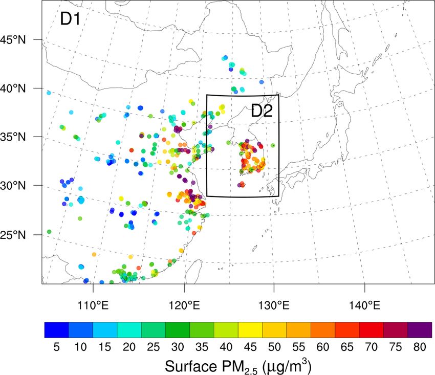
1776                                                     S. Ha: Aerosol data assimilation using the RACM/MADE-VBS scheme

Figure 4. The horizontal length scales of the same species as in Fig. 3.

anthropogenic primary aerosol (antha), marine aerosol con-                 terpolation (e.g., bilinear interpolation) of the corresponding
centration (seas), and soil-derived aerosol particles such as              variable at the lowest model level.
dust (soila) – into the simulated PM2.5 . But in the concur-
rent assimilation of PM10 and PM2.5 , the residuals from                   2.3   Observation processing and measurement errors
PM10 –PM2.5 are assimilated as a sum of three coarse-mode
aerosols, following Peng et al. (2018) and Sun et al. (2020).              In this study, hourly surface observations of six major pol-
  Unlike the aerosol analysis that has to update dozens of                 lutants (PM2.5 , PM10 , SO2 , NO2 , O3 , and CO) are used
aerosol species (e.g., unobserved variables) from PM con-                  from 379 Korean sites operated by the NIER (http://www.
centrations, the assimilation of trace gases is straightforward            airkorea.or.kr, last access: 21 December 2020) and around
because each gas species is the model prognostic variable in               1600 sites from the China National Environmental Moni-
most chemical options. Thus, the control variables are sim-                toring Center (CNEMC; http://www.cnemc.cn, last access:
ply expanded for four gas species (SO2 , NO2 , O3 , and CO),               21 December 2020) during the KORUS-AQ period. All the
and the observation operator becomes a simple horizontal in-               gas species measured in Korean stations have the same

Geosci. Model Dev., 15, 1769–1788, 2022                                                    https://doi.org/10.5194/gmd-15-1769-2022
S. Ha: Aerosol data assimilation using the RACM/MADE-VBS scheme                                                                1777

Table 2. A list of new namelist parameters in WRFDA.

                                      Namelist options              Description
                      &wrfvar7        chem_cv_options = 108         racm_soa_vbs_kpp
                      &wrfvarchem     use_chemic_surfobs = .true.   chemical DA
                      &chem           chemicda_opt = 1              1 = PM2.5
                                                                    2 = PM10
                                                                    3 = PM2.5 and PM10
                                                                    4 = all (PM2.5 , PM10 , SO2 , NO2 , O3 , CO)
                                                                    5 = gas only (SO2 , NO2 , O3 , CO)

ppmv unit as in WRF-Chem, but all the Chinese sites re-                In this 3D-Var analysis, observation errors are assumed
port the data in µg m−3 , requiring a unit conversion as part       uncorrelated such that the observation error covariance ma-
of observation processing. Using the molecular weight of            trix R in Eq. (1) becomes diagonal with the observation error
each gas species (wgas ) and the molar volume of a gas              standard deviations as diagonal elements. For the gas species,
(Vm = 22.4 L mol−1 ) at 1 standard temperature and pres-            the observation error is simply assigned as 10 % of the ob-
sure (STP), the unit of the Chinese data is converted as            served value regardless of the location. For surface PM con-
[ppmv] = [µg m−3 ] × Vm /wgas /1000.                                centrations, the observation error is estimated as a sum of
   As the surface stations are mostly concentrated in the large     the measurement
                                                                             p         error (o ) and the representative error (r )
cities, the hourly data that belong to the same 9 km model          as x = o 2 + r 2 , following Elbern et al. (2007). The mea-
grid are randomly split for assimilation and verification; each     surement error increases linearly with the observed value (xo )
dataset is then averaged over each grid. As a result, 279 Ko-       as o = 1.5+0.0075·x q o , while the representative error is for-
rean sites are averaged into 219 stations (or grids) for as-        mulated as r = γ o 1xL , where γ is set to be 0.5, 1x is grid
similation, while the other 100 sites are averaged to 71 inde-
                                                                    spacing (here, 27 km for domain 1 and 9 km for domain 2),
pendent observations for evaluation over South Korea. The
                                                                    and the scaling factor L is defined as 3 km, as in Ha et al.
Chinese data have a lot of missing values, especially for the
                                                                    (2020).
period of heavy pollution events (24–26 May 2016), and be-
cause the verification is made over Korean sites only, they
are used without such processing.                                   3   Results from cycling experiments
   Data quality control (QC) is done by setting maximum
thresholds of observation values and innovations ((o − f)’s)        A month-long cycling experiment is conducted, assimilating
during the assimilation procedure. Surface PM2.5 and PM10           all the surface observations for six pollutants (PM2.5 , PM10 ,
observations are rejected when they are greater than 300,           SO2 , NO2 , O3 , and CO) (e.g., chemicda_opt = 4) in both do-
500 µg m−3 , respectively, or are different from their model        mains every 6 h. The baseline experiment (“NODA”) is first
equivalent (e.g., H(x b )) by more than 100 µg m−3 . Gas            conducted, recycling 6 h forecasts from the previous cycle.
species are also checked with the maximum threshold of 2,           The background error statistics are computed from the ex-
2, 2, and 20 ppmv for the observed SO2 , NO2 , O3 , and CO,         tended forecasts (e.g., up to 48 h) in NODA. Then, the DA ex-
respectively. They are also rejected based on the threshold of      periment assimilates all the observations to update the analy-
0.2 ppmv for the innovations.                                       sis every 6 h based on the background error covariance, using
   Gas-phase pollutants on the ground are assimilated to-           the same input data and the same lateral boundary conditions
gether, as opposed to individual species, using the cor-            for both meteorological and chemical fields as in NODA.
responding model variables as their analysis (or control)              The UM global forecasts are initialized from the UM anal-
variables. Before assimilation, observations for all the gas        ysis at 18:00 UTC every day so that the UM global analy-
species are processed to have the same ppmv unit as the             sis is used for 18:00 UTC cycles, while the following 6–18 h
model variables, as needed.                                         UM forecasts are employed at 00:00–12:00 UTC cycles the
   For the new assimilation capability, several new parame-         next day, respectively. The UM simulations run by KMA de-
ters are added to namelist.input in WRF-Chem, as summa-             fine surface fields at 1.5 m and the soil moisture content at
rized in Table 2. To demonstrate the capability of all the new      0–0.1, 0.1–0.35, 0.35–1.0, and 1–3 m soil layers in units of
observation operators (that are independent of each other),         [kg m−2 TS−1 ], where TS indicates the thickness of each soil
this study only presents the simultaneous assimilation of all       layer. To ungrib the data correctly, the Vtable and the ungrib
six pollutants using chemicda_opt = 4, as listed in Table 2.        source codes in WPS are modified accordingly.

https://doi.org/10.5194/gmd-15-1769-2022                                               Geosci. Model Dev., 15, 1769–1788, 2022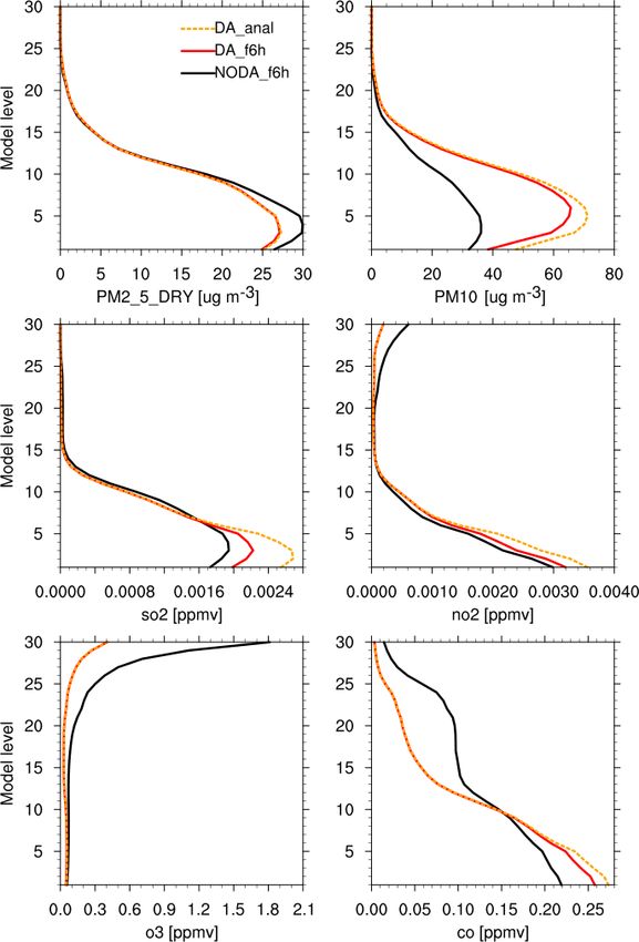
1778 S. Ha: Aerosol data assimilation using the RACM/MADE-VBS scheme
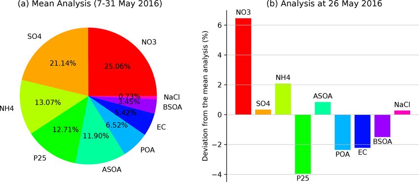
The MADE-VBS aerosol parameterization has been re-
ported to simulate the chemical composition over the East
Asian region reasonably well (Lee et al., 2020; Saide et al.,
2020). As shown in Fig. 8a, the surface PM2.5 analysis
is dominated by nitrates (NO3 ), sulfate (SO4 ), ammonium
(NH4 ), unspeciated PM2.5 , and anthropogenic secondary or-
ganic aerosols (ASOA) in Seoul, South Korea (in that or-
der), consistent with the background error estimates shown
in Fig. 2. Compared to the analysis averaged over the whole
evaluation period, the analysis in the heavy pollution event
on 26 May 2016 (Fig. 8b) indicates that major constituents’
contributions further increase, particularly by nitrate. Due to
the limited information content of atmospheric composition
measurements as well as the scarcity of such observations, it
Figure 5. Time series of hourly PM2.5 concentration on the ground. is hard to evaluate the fractional aerosol contribution by all
The baseline experiment (“NODA”) is plotted in black, while the the species defined in the MADE-VBS scheme. Hence, these
DA experiment with the analysis every 6 h in red. Observations av- figures are presented only to show the aerosol composition
eraged over all the evaluated stations in South Korea are marked as
represented by the analysis using the aerosol chemistry and
blue dots, enclosed with the shaded area in light blue for the stan-
dard deviation in observations.
how it changes when surface PM2.5 concentrations are high
due to long-range transport of air pollutants. In the WRFDA
system, several tuning parameters (such as var_scaling and
Figure 5 depicts the time series of hourly surface PM2.5 len_scaling) are supported for further adjustments of each
concentrations, averaged over 71 evaluation sites in South aerosol species, as needed. Using the default setting (e.g.,
Korea for the last week of May 2016 with heavy pollution without tuning), the fractional contribution is not substan-
events. Observations are marked in blue dots, and the hourly tially changed by assimilation in this particular case study.
forecasts in DA and NODA are drawn in solid red and black The overall composition with major constituents seems con-
lines, respectively. The NODA experiment concatenates 0– sistent with those from previous studies (Jo et al., 2020; Tian
6 h forecasts every cycle, while DA presents the analysis for et al., 2019).
every 6 and 1–5 h forecasts for other times. The 3D-Var anal- Figure 9 presents the horizontal distribution of analysis
ysis and the subsequent forecasts in DA follow the observa- increments (equal to the difference between the analysis
tions closely, but without data assimilation, 0–6 h forecasts in and the background) in the assimilated variables at the low-
NODA largely deviate from the measurements, even beyond est model level, averaged for the evaluation period. Surface
the observation uncertainty across stations (shaded in light PM2.5 concentrations are reduced by assimilation, especially
blue). over central eastern China (along 30◦ N), indicating that they
Figures 6 and 7 illustrate observation minus background were mostly overpredicted in background forecasts, likely
(omb; dotted gray line) and observation minus analysis (oma; due to the systematic overestimation of anthropogenic emis-
solid black line) in DA, as a time series of surface PM sion data. Given that air pollutants in the emission data con-
concentrations and gas species, respectively, for the entire stitute the majority of the precursors of PM2.5 pollution, sur-
month. The total number of observations (blue dots in Fig. 6) face PM2.5 concentrations could strongly depend on emis-
varies from cycle to cycle, but the time series of omb and sions, which might have led to the overestimation in the
oma indicates that the analysis system gets spun up quickly background forecasts (Chen et al., 2019). Therefore, the as-
(with the steady trend of oma) and runs reliably throughout similation of surface PM2.5 tends to counteract the overes-
the month-long period with the analyses closer to observa- timation driven by the emission data over China. On the
tions than background forecasts for all six pollutants. The contrary, PM10 concentrations are predominantly enhanced
number of observations in trace gases is omitted in Fig. 7 be- by assimilation over most areas, presumably because coarse-
cause it is very similar to that of PM observations, and the mode aerosols might not be sufficiently described in both the
omb in gas species is greatly fluctuating with cycles. Such emission data (through “E_PM_10”) and the model estimate.
large oscillations of omb and large differences between anal- Among the coarse-mode species, dust aerosols (soila) show
ysis and background are often attributable to the consider- the most significant analysis increments over the Jing–Jin–
able errors in the forecast model and/or forcing parameters, Ji (an abbreviation of the Chinese names of Beijing, Tianjin,
which prompt the model state to return to its own equilib- and Hebei) metropolitan region (not shown). On the other
rium quickly (e.g., within 6 h). For the rest of the figures, the hand, the analysis does not make meaningful changes in SO2
evaluation is made only for 7–31 May 2016, discarding the and NO2 but tends to decrease ozone and increase carbon
first week of cycling as a spin-up period. monoxide over South Korea.
Geosci. Model Dev., 15, 1769–1788, 2022 https://doi.org/10.5194/gmd-15-1769-2022S. Ha: Aerosol data assimilation using the RACM/MADE-VBS scheme 1779 Figure 6. Time series of observation minus background (omb; dotted gray line) and observation minus analysis (oma; solid black line) in surface PM2.5 (a) and PM10 (b) in the “DA” experiment, in terms of root-mean-square error over all the stations assimilated in domain 1 at each cycle. The averages over cycles are shown in the legend, and the total number of stations at each cycle is marked in blue dots with the y axis on the right. Figure 10 examines how the vertical distribution of aerosol PM10 displays relatively large discrepancies between the two species systematically changes with the assimilation over do- and even bigger differences between NODA and DA, mainly main 2. Even if only the surface observations were assimi- due to the large changes in soila, as shown in the previous lated, the entire boundary layer is affected by continuous cy- figure. Systematic disparities between observations and the cling, based on the aerosol forecast error structure. The DA model estimates typically imply the deficiencies in the model experiment mainly reduces most aerosol species contribut- simulation and/or the forcing parameters. As the focus of this ing to PM2.5 in the boundary layer. But soil-derived dust and study is the prediction of surface PM2.5 concentrations, no sea salt aerosols are significantly increased in the low tro- further investigation is made on the systematic errors in PM10 posphere, due to their large standard deviations and eigen- simulations in this study. But generally, the larger the model values estimated in the background error covariance. These error gets, the harder it is to make an optimal solution in the coarse-mode variables could be also affected by weather con- analysis. On the other hand, SO2 and NO2 near the surface ditions to a greater extent as they could be more sensitive to are slightly increased by assimilation over domain 2, which the large-scale advection like low-level jets. The role of me- does not last for 6 h because of their short lifetime. While teorological fields or their interactions with aerosols will be the changes in the vertical structure of those two fields are examined in the context of concurrent data assimilation of confined to the boundary layer, ozone and carbon monoxide chemical and meteorological observations in the following experience the adjustments for the entire profile through the study. cycling. The reduction of PM2.5 and the large increase of PM10 in Figure 12 illustrates the time series of rms and bias errors the boundary layer, as shown in Fig. 11, are consistent with of 0–48 h forecasts with respect to independent PM2.5 obser- previous results. PM2.5 shows that the analysis (orange) and vations at the surface. The large initial errors in NODA imply the following 6 h forecast (red) are not much different in the that aerosol species are not properly initialized without as- climatological sense (e.g., mean over time and space). But similation, even if they are recycled every 6 h for the whole https://doi.org/10.5194/gmd-15-1769-2022 Geosci. Model Dev., 15, 1769–1788, 2022
1780                                                  S. Ha: Aerosol data assimilation using the RACM/MADE-VBS scheme

Figure 7. Same as Fig. 6 but for gas species.

month. With data assimilation, initial conditions in the DA         species except for carbon monoxide, partly due to the model
experiment are substantially improved over both domains,            errors and partly due to the observation errors that might need
leading to smaller forecast errors throughout 48 h forecasts.       to be further adjusted for better results.
In domain 1, a large overestimation in NODA is significantly           The forecast errors depicted in Fig. 12 are dominated
reduced by assimilation, but the positive bias remains for          by moderate (or clear-sky) cases in Korea, but air qual-
48 h. In domain 2, the systematic bias is mostly corrected          ity forecasting becomes more crucial for heavy pollution
in DA up to 36 h forecasts, and the RMSEs are consistently          events, making the categorical forecast verification impor-
small compared to NODA. The forecast errors are mostly              tant in a practical sense. Table 4 categorizes four different
distinguishable for the first 24 h, and the analysis impact typi-   events based on hourly surface concentrations in six pollu-
cally lasts no longer than 6 h in trace gases like NO2 and SO2 ,    tants, and Table 5 defines categorical forecasts for different
24 h forecast mean errors are thus summarized in Table 3 for        air pollution events. Figure 13 highlights the forecast accu-
all six pollutants. Compared to the baseline run (NODA), the        racy for categorized events, verified against independent ob-
DA experiment systematically improves surface PM2.5 fore-           servations, based on the formulae described below.
casts in both domains, with the RMSEs decreased by 26 %
and 20 % over domains 1 and 2, respectively. The RMSEs of
PM10 are reduced only by ∼ 14 % in DA, but the systematic                                  a1 + b2 + c3 + d4
                                                                    Overall_Accuracy (%) =                   × 100             (5)
underestimation gets mostly diminished over both domains.                                          N
The assimilation is not very effective in the prediction of gas                                   c3 + d4
                                                                    High_Pollution_Accuracy (%) =          × 100               (6)
                                                                                                  III + IV

Geosci. Model Dev., 15, 1769–1788, 2022                                             https://doi.org/10.5194/gmd-15-1769-2022
S. Ha: Aerosol data assimilation using the RACM/MADE-VBS scheme 1781
Figure 8. (a) Pie chart showing the percentage contribution by aerosol species in Seoul, South Korea, in the analysis averaged over 97 cycles
from 00:00 UTC on 7 May to 00:00 UTC on 31 May 2016 and (b) deviations from the mean analysis in the analysis at 00:00 UTC on 26 May
2016 over domain 2 in the DA experiment. Surface PM2.5 consists of aerosol sulfate (SO4 ; so4ai and so4aj), ammonium (NH4 ; nh4ai and
nh4aj), nitrate (NO3 ; no3ai and no3aj), primary organic matter (POA; orgpai and orgpaj), elemental carbon (EC; eci and ecj), unspeciated
PM2.5 (P25; p25ai and p25aj), sodium chloride (NaCl; naai, naaj, clai, and claj), and four-bin anthropogenic and biogenic secondary organic
aerosol (ASOA and BSOA, respectively) at the lowest model level.
Table 3. The RMSE and bias errors of 24 h forecasts in NODA and rors usually grow with time due to the model uncertainty, this
DA experiments. means that the forcing parameters consistently constrain the
chemical forecasting. With data assimilation (red), the ini-
RMSE Bias tial accuracy gets doubled up in both domains (up to 80 %),
D1 D2 D1 D2 even for high-pollution cases. But the benefit of the anal-
ysis quickly disappears with time, implying the challenges
PM2.5 NODA 42.8 21.3 15.4 2.5 with chemical data assimilation using the 3D-Var technique
DA 31.6 17.0 8.4 0.0 and large uncertainties in aerosol simulations. Note that the
PM10 NODA 53.4 33.0 −9.6 −13.9 DA algorithm used here cannot produce an optimal solu-
DA 46.1 28.2 −0.7 −1.9 tion when there are significant errors in the model and/or the
SO2 NODA 0.016 0.006 0.007 0.001
forcing parameters as the strong-constraint variational sys-
DA 0.015 0.006 0.007 0.001 tem assumes a perfect model in the optimization. As Boc-
quet et al. (2015) pointed out, even with the improved anal-
NO2 NODA 0.018 0.001 0.017 −0.001 ysis, it is hard to compete with forcing parameters such as
DA 0.017 0.000 0.017 −0.003 emissions by which the chemical transport model is strongly
O3 NODA 0.023 0.007 0.02 0.006 driven, making the chemical analysis impact typically lim-
DA 0.022 −0.006 0.02 −0.004 ited to the first-day forecasts. The results shown here are
consistent with previous studies, illustrating that most of the
CO NODA 0.662 −0.209 0.277 −0.228
DA 0.642 −0.182 0.249 −0.184 benefits from data assimilation are limited to the first 24 h
forecasts, although the overall forecast accuracy in DA still
remains higher than NODA up to 48 h. In domain 2, due to
II the small sample size, the forecast accuracy for high con-
False_Alarm (%) = × 100, (7) centrations is not as consistent (and smooth) as in domain 1,
II + IV
and the results may not be statistically significant. But the
where I = a1+a2+b1+b2, II = c1+c2+d1+d2, III = a3+ false alarm rates for all events are also reduced for 0–24 h
a4+b3+b4, IV = c3+c4+d3+d4, and N = I+II+III+IV. forecasts, indicating that the assimilation systematically im-
The air quality forecasting operated by the NIER in South proves the 9 km simulations (in D2).
Korea is currently evaluated in the same way daily, except for
daily mean values (rather than hourly averages). The forecast
accuracy rates defined here can be considered as skill scores 4 Conclusions and discussion
for categorized events so that the higher they are, the better
they become. First of all, NODA shows very stable accuracy This study introduced a new extended version of the WRFDA
rates between 40 % and 50 % for all events. As forecast er- 3D-Var analysis system for the RACM chemistry and the
https://doi.org/10.5194/gmd-15-1769-2022 Geosci. Model Dev., 15, 1769–1788, 20221782 S. Ha: Aerosol data assimilation using the RACM/MADE-VBS scheme
Figure 9. Horizontal distribution of the analysis increments in particulate matter concentrations and four gas species at the lowest model
level over domain 1 in the DA experiment, averaged for 7–31 May 2016. The domain average is shown in the top right corner of each panel.
Table 4. Air quality index values, as defined in the NIER in Korea.
Concentration (hourly) Good Moderate Unhealthy Very unhealthy
PM2.5 [µg m−3 ] 15 35 75 > 75
PM10 [µg m−3 ] 30 80 150 > 150
SO2 [ppmv] 0.02 0.05 0.15 > 0.15
NO2 [ppmv] 0.03 0.06 0.20 > 0.20
O3 [ppmv] 0.03 0.09 0.15 > 0.15
CO [ppmv] 2 9 15 > 15
Geosci. Model Dev., 15, 1769–1788, 2022 https://doi.org/10.5194/gmd-15-1769-2022S. Ha: Aerosol data assimilation using the RACM/MADE-VBS scheme 1783
Figure 10. Vertical profile of aerosol species ([µg kg−1 ]) averaged over domain 2. The 6 h forecasts in NODA (black) and DA (red) are
depicted with solid lines, while the analyses in DA are indicated by the dotted orange line.
Table 5. Categorical forecasts for different air pollution events.
Category Forecast
Good Moderate Unhealthy Very unhealthy
Observation Good a1 b1 c1 d1
Moderate a2 b2 c2 d2
Unhealthy a3 b3 c3 d3
Very unhealthy a4 b4 c4 d4
https://doi.org/10.5194/gmd-15-1769-2022 Geosci. Model Dev., 15, 1769–1788, 20221784 S. Ha: Aerosol data assimilation using the RACM/MADE-VBS scheme
Figure 12. Time series of (a, b) root-mean-square error (RMSE)
and (c, d) bias as (forecast minus observation) in surface PM2.5 con-
centration of the hourly forecasts from the analysis at 00:00 UTC
from 7 to 31 May 2016. The left panels (a, c) show the errors of
forecasts at 27 km resolution verified against 1188 stations over do-
main 1, and the right panels (b, d) present the 9 km forecast errors
with respect to surface PM2.5 observations from 71 independent
stations in Korea.
the Korean Peninsula. The analysis does not make meaning-
ful changes in SO2 and NO2 because of their short lifetime.
The month-long cycling experiments confirmed that the
Figure 11. Same as Fig. 10 but for six pollutants assimilated in DA. aerosol assimilation could improve air quality forecasts for
24 h, verified against independent observations. The im-
provements were evident even in the heavy pollution events
MADE-VBS aerosol parameterization (chem_opt = 108) in (24–26 May 2016) over South Korea, suggesting that the
the WRF-Chem forecast model. It is demonstrated that the new system can be useful for predicting exceedance and
new analysis capability is successfully implemented for sur- non-exceedance events. Given the lack of interoperability be-
face observations for six pollutants (PM2.5 , PM10 , SO2 , NO2 , tween chemical parameterization schemes, these results val-
O3 , and CO) through the cycling experiments over the East idate that the MADE/VBS aerosol scheme can improve air
Asian region for May 2016. quality forecasting in the context of chemical weather cy-
As specified in the background error covariance estima- cling, especially over the East Asian region. The new codes
tion, the assimilation of the ground measurements affects the developed here will be included in the next release of the
entire boundary layer and the surrounding area (up to four WRFDA system.
grid points from the observation sites in domain 2). In the as- Even with the successful demonstration of the new imple-
similation of surface PM concentrations, each aerosol species mentation, however, the 3D-Var analysis system can be fur-
is adjusted according to its background errors, contributing to ther improved or examined to maximize the impact of chem-
the atmospheric composition differently. Inorganic aerosols ical observations. In an effort to optimize the system design,
in the accumulation mode (no3aj, so4aj, and nh4aj), the ma- conventional weather data were assimilated at the same time,
jor constituents of PM2.5 in the RACM/MADE-VBS scheme, and chemical boundary conditions were updated every 6 h.
are adjusted more than the Aitken-mode aerosols, spread- Many processes and inputs (e.g., emissions) depend on me-
ing more widely in both horizontal and vertical. Dust and teorological conditions, and the large-scale chemical forcing
sea salt aerosols in the coarse mode significantly increase in can affect the quality of background forecasts, but their roles
the boundary layer, leading to a substantial increase in PM10 on aerosol prediction were not examined, focusing on the
concentrations on the ground over East Asia. In the assimila- demonstration of the new development. Large uncertainties
tion of trace gases, carbon monoxide is mainly increased near in the forecast model and the emission data were also not ex-
the surface, while the surface ozone slightly decreases over amined, as well as the observation errors that may need to be
Geosci. Model Dev., 15, 1769–1788, 2022 https://doi.org/10.5194/gmd-15-1769-2022S. Ha: Aerosol data assimilation using the RACM/MADE-VBS scheme 1785
Figure 13. Same as Fig. 12 but for the forecast accuracy (%) for categorized events, as defined in Tables 4 and 5. The 48 h mean forecast
accuracy of each experiment is shown in the legend.
tuned, especially for trace gases. Those important aspects are Code and data availability. The WRF-Chem v3.9.1 codes
left behind for future studies. A more appropriate choice of are freely available from https://www2.mmm.ucar.edu/wrf/
control variables, for example, can enhance the conditioning users/download/get_source.html (NCAR, 2021). The WRFDA
of the 3D-Var problem (Courtier and Talagrand, 1990). The source codes developed for this study and the WPS codes
observation operator used in this study treated each aerosol modified for the UM grib data can be downloaded from
https://doi.org/10.5281/zenodo.4594671 (Ha, 2021). Real-time air
species in each mode as an individual control variable, but
quality observations are available at http://www.airkorea.or.kr/
because the Aitken-mode variables contributed to the partic-
(Air Korea, 2020) for Korean sites and at http://www.cnemc.cn
ulate matter concentrations only for about 10 %, it might be (China National Environmental Monitoring Centre, 2020) for
worth trying to reduce the total number of control variables Chinese stations. The NCEP prepbufr data are archived and
by either using major constituents or combining Aitken and available at the National Center for Atmospheric Reserach
accumulation modes for each species. (https://doi.org/10.5065/Z83F-N512, National Centers for Envi-
The error cross correlations between meteorological vari- ronmental Prediction et al., 2008). CAM-Chem model outputs
ables and chemical species or between chemical species for lateral boundary condition files can be downloaded from
could not be specified in the current variational data assim- https://www.acom.ucar.edu/cam-chem/cam-chem.shtml (last ac-
ilation framework but might also play a significant role in cess: 28 December 2020, Buchholz et al., 2019). The WRF-Chem
improving air quality forecasting, particularly for long-range preprocessor tools such as mozbc and megan_bio_emiss are
available at https://www.acom.ucar.edu/wrf-chem/download.shtml
transport of air pollutants that often cause heavy pollution
(ACOM/NCAR, 2020).
events over Korea. For a dynamical estimation of such cross
correlations, ensemble-based methods should be introduced
(Bocquet et al., 2015; Miyazaki et al., 2020; Sandu and Chai, Competing interests. The contact author has declared that there are
2011). no competing interests.
https://doi.org/10.5194/gmd-15-1769-2022 Geosci. Model Dev., 15, 1769–1788, 2022You can also read