Improved representation of river runoff in Estimating the Circulation and Climate of the Ocean Version 4 (ECCOv4) simulations: implementation ...
←
→
Page content transcription
If your browser does not render page correctly, please read the page content below
Geosci. Model Dev., 14, 1801–1819, 2021
https://doi.org/10.5194/gmd-14-1801-2021
© Author(s) 2021. This work is distributed under
the Creative Commons Attribution 4.0 License.

Improved representation of river runoff in Estimating the
Circulation and Climate of the Ocean Version 4 (ECCOv4)
simulations: implementation, evaluation, and
impacts to coastal plume regions
Yang Feng1,2,3 , Dimitris Menemenlis4 , Huijie Xue1,2 , Hong Zhang4 , Dustin Carroll4,5 , Yan Du1,2,6 , and Hui Wu7
1 State Key Laboratory of Tropical Oceanography, South China Sea Institute of Oceanology & Institution of South China Sea
Ecology and Environmental Engineering, Chinese Academy of Science, Guangzhou, China
2 Southern Marine Science and Engineering Guangdong Laboratory, Guangzhou, China
3 Guangdong Key Laboratory of Ocean Remote Sensing, South China Sea Institute of Oceanology,

Chinese Academy of Sciences, Guangzhou, China
4 Jet Propulsion Laboratory, California Institute of Technology, Pasadena, California, USA
5 Moss Landing Marine Laboratories, San José State University, Moss Landing, California, USA
6 College of Marine Science, University of Chinese Academy of Sciences, Guangzhou, China
7 State Key Laboratory of Estuarine and Coastal Research, East China Normal University, Shanghai, China

Correspondence: Yang Feng (yfeng1982@126.com)

Received: 24 September 2020 – Discussion started: 27 October 2020
Revised: 13 February 2021 – Accepted: 21 February 2021 – Published: 1 April 2021

Abstract. In this study, we improve the representation of         ally, we find that the impacts of increasing model resolution
global river runoff in the Estimating the Circulation and Cli-    from the intermediate-resolution LLC270 grid to the high-
mate of the Ocean Version 4 (ECCOv4) framework, allow-            resolution LLC540 grid are regionally dependent. The Mis-
ing for a more realistic treatment of coastal plume dynamics.     sissippi River Plume is more sensitive than other regions,
We use a suite of experiments to explore the sensitivity of       possibly because the wider and shallower Texas–Louisiana
coastal plume regions to runoff forcing, model grid resolu-       shelf drives a stronger baroclinic effect, as well as relatively
tion, and grid type. The results show that simulated sea sur-     weak sub-grid vertical mixing and adjustment in this region.
face salinity (SSS) is reduced as the model grid resolution in-   Since rivers deliver large amounts of freshwater and anthro-
creases. Compared to Soil Moisture Active Passive (SMAP)          pogenic materials to coastal regions, improving the represen-
observations, simulated SSS is closest to SMAP when us-           tation of river runoff in global, high-resolution models will
ing daily, point-source runoff (DPR) and the intermediate-        advance studies of coastal hypoxia, carbon cycling, and re-
resolution LLC270 grid. The Willmott skill score, which           gional weather and climate and will ultimately help to predict
quantifies agreement between models and SMAP, yields up           land–ocean–atmospheric feedbacks seamlessly in the next
to 0.92 for large rivers such as the Amazon. There was no         generation of Earth system models.
major difference in SSS for tropical and temperate coastal
rivers when the model grid type was changed from the
ECCO v4 latitude–longitude–polar-cap grid to the ECCO2
cube–sphere grid. We also found that using DPR forcing            1   Introduction
and increasing model resolution from the coarse-resolution
LLC90 grid to the intermediate-resolution LLC270 grid el-         Coastal plume regions represent a small fraction of Earth’s
evated the river plume area, volume, stabilized the stratifi-     surface and are an active component in global cycling of car-
cation and shoal the mixed layer depth (MLD). Addition-           bon and nutrients (Bourgeois et al., 2016; Carroll et al., 2020;

Published by Copernicus Publications on behalf of the European Geosciences Union.
1802                                                            Y. Feng et al.: Improved representation of ECCO river runoff

Fennel et al., 2019; Lacroix et al., 2020; Landschützer et al.,     2002; Stammer et al., 2004). Recent ECCO efforts have been
2020; Roobaert et al., 2019). Recent satellite-based observa-       extended to address the global-ocean estimates of pCO2 and
tions with quasi-global coverage have been greatly improved         air–sea carbon exchange (Carroll et al., 2020), and model
to monitor sea surface salinity (SSS), a key tracer for track-      resolution as fine as 1 km has been promoted globally to in-
ing the river plumes. The European Space Agency (ESA)               vestigate mesoscale-to-submesoscale dynamics in the open
Soil Measure and Ocean Salinity (SMOS; Mecklenburg et               ocean (Su et al., 2018). However, current ECCO lacks repre-
al., 2012) with 33 km–10 d space–time gridding and National         sentation of coastal interfaces and related feedbacks limiting
Aeronautics and Space Administration (NASA) Soil Mois-              their predictability to global climate change, and this may
ture Active Passive (SMAP) missions with 40 km–8 d space–           further impede our ability to make informed resource man-
time gridding are acquiring SSS observations with sufficient        agement decisions. In this study, we improve the representa-
resolution to track the plume pathways and evaluate coastal         tion of river runoff in the ECCO and systematically evaluate
plume dynamics (Fournier et al., 2016a, b, 2017a, b, 2019;          model performance in reproducing SSS within the vicinity
Gierach et al., 2013; Liao et al., 2020). To date, however,         of large tropical and temperate river mouths. We also investi-
the coastal plume regions have not been explicitly resolved         gate the impact of runoff forcing, model grid resolution, and
in most global ocean general circulation models (OGCMs),            grid type on coastal dynamics and critical physical properties
Earth system models (ESMs), and Global Ocean Data As-               near the plume regions. The goal of this work is to provide a
similation System (GODAS) products (Ward et al., 2020).             comprehensive sensitivity analysis of runoff forcing in mul-
As a result, the plume region produced by OGCMs, ESMs,              tiple simulations, which will aid in the development of global
and GODAS are not consistent with satellite observations.           ECCO that more robustly reflecting the land–ocean aquatic
For example, Fournier et al. (2016a) found that the 1/12◦           continuum (LOAC).
global circulation Hybrid Coordinate Ocean Model (HY-                  The paper is organized as follows. Section 2 briefly intro-
COM) did not accurately capture SSS during extreme flood            duces the ECCO model and the various runoff forcing meth-
events in the northern Gulf of Mexico. Denamiel et al. (2013)       ods used in this study. Section 3 provides a comprehensive
found that the Congo River nearshore SSS in global HYCOM            evaluation of model sensitivity to horizontal grid resolution
was underestimated compared to other regional simulations,          and river forcing. Section 4 discusses the sensitivity of plume
even though the models had comparable horizontal grid res-          properties and coastal stratification. Results are summarized
olution. Santini and Caporaso (2018) suggested that most            in Sect. 5.
CMIP5 models might lack skill in representing the Congo
River Basin runoff and SSS in the vicinity of river mouths.
Most OGCMs, ESMs, and GODAS products usually had                    2     Methods
large grid cells; a few cells may encompass the entire plume.
As a result, water delivered to the cells are fully mixed and       2.1    ECCO simulations and representation of river
diluted and therefore cannot accommodate the complex dy-                   runoff
namics. Additionally, riverine freshwater input to the ocean
is forced in the top model layer over a pre-determined sur-         In this study, we employ the Massachusetts Institute of Tech-
face area in the vicinity of river mouths with climatologi-         nology general circulation model (MITgcm; Marshall et al.,
cal signal; thus the system disturbance by extreme weather          1997) in a number of model configurations that have been
events, e.g., floods and droughts, cannot been explicitly re-       developed for the ECCO project (Menemenlis et al., 2005;
solved (Griffies et al., 2005; Tseng et al., 2016). Finally, vir-   Forget et al., 2015; Zhang et al., 2018). The ECCO MIT-
tual salt fluxes (VSFs) have been widely employed, where            gcm configurations that we use herein solve the hydrostatic,
freshwater affects salinity without a change in mass or vol-        Boussinesq equations on either cube–sphere (CS; Adcroft
ume flux (Bentsen et al., 2013; Halliwell, 2004; Timmer-            et al., 2004) or latitude–longitude–polar-cap (LLC; Forget
mann et al., 2009; Volodin et al., 2010). The above model           et al., 2015) grids. The cube–sphere configuration that we
configurations may limit the representation of coastal plume        use is the so-called CS510 grid, which was developed for the
regions in global-scale models.                                     ECCO2 project (Menemenlis et al., 2008), consists of 6 faces
   Estimating the Circulation and Climate of the Ocean              with 510 × 510 dimension, and has quasi-homogeneous hor-
(ECCO) is a data-assimilating model that uses observational         izontal grid spacing of 20 km. We also consider three differ-
data to make the best possible estimates of ocean circula-          ent LLC grid configurations: LLC90, LLC270, and LLC540,
tion and its role in climate. The model takes the cube–sphere       which have, respectively, 1◦ , 1/3◦ , and 1/6◦ nominal hori-
(ECCO2) to latitude–longitude–polar-cap (ECCOv4) grids              zontal grid spacing. The LLC grids are aligned with lines of
for global application. Like most OGCMs, ESMs, and GO-              latitude and longitude between 70◦ S and 57◦ N and are lo-
DAS products, the current ECCO routes riverine freshwa-             cally isotropic with grid spacing varying with latitude. In the
ter from land directly to the ocean by taking observed river        tropics, the LLC grid is refined in the meridional direction to
runoff as seasonal climatology mass flux over the top of sev-       better resolve zonal currents. At high latitudes, the LLC grid
eral surface grid cells near the river mouths (Fekete et al.,       is adapted to a two-dimensional conforming mapping algo-

Geosci. Model Dev., 14, 1801–1819, 2021                                             https://doi.org/10.5194/gmd-14-1801-2021
Y. Feng et al.: Improved representation of ECCO river runoff                                                                 1803

rithm for spherical geometry. For our experiments, we use           2.2   Sensitivity experiments
LLC# horizontal grids, where the # is the number of points
along one-quarter of the Equator. Therefore, LLC90 means            We first run seven experiments, derived from the EC-
360 grid points circle the Equator. The model has 50 ver-           COv4 setup, to test the sensitivity of SSS in the vicin-
tical z levels; vertical resolution is 10 m in the top 7 levels     ity of large river mouths to ECCOv4 model grid resolu-
and telescopes to 450 m at depth. This setup was the same           tion and runoff forcing (Table 1). The LLC90, LLC270,
for all designed experiments. We use a third-order, direct-         and LLC540 correspond to coarse (1◦ – ∼ 100 km), inter-
space–time (DST-3) advection scheme, while vertical advec-          mediate (1/3◦ – ∼ 40 km), and high (1/6◦ – ∼ 20 km) res-
tion uses an implicit third-order upwind scheme. Vertical           olution from low latitudes to mid-latitudes. LLC90C and
mixing is parameterized using the Gaspar–Grégoris–Lefevre           LLC270C are forced by monthly climatological runoff from
(GGL) mixing-layer turbulence closure and convective ad-            Fekete et al. (2002). The runoff has a spatial resolution of
justment scheme (Gaspar et al., 1990). Lateral eddy viscosity       ∼ 1◦ and has been linearly interpolated to each grid cell.
in ECCOv4 is harmonic, with a coefficient of 0.005L2 /1t,           Therefore, runoff may be fluxed into a single grid cell in
where L is the grid spacing in meters and 1t = 3600 s. De-          the coarse-resolution run and over several grid cells in the
pending on location, the resulting eddy viscosity varies from       high-resolution run. The twin experiments, LLC90R and
∼ 103 to ∼ 1.6 × 10⁴ m2 s−1 . Additional sources of dissipa-        LLC270R, as well as the highest resolution run LLC540R,
tion in ECCOv4 are from harmonic vertical viscosity and             use the Japanese 55-year atmospheric reanalysis (JRA55-
quadratic bottom drag, along with contributions from the ver-       DO) river forcing dataset (Suzuki et al., 2017; Tsujino et
tical mixing parameterization. A detailed description of EC-        al., 2018). JRA55-DO includes daily river runoff gener-
COv4 is provided in Forget et al. (2015).                           ated by running a global hydrodynamic model forced by
   ECCOv4 uses natural boundary conditions for the surface          adjusted land-surface runoff. Compared to the Fekete EC-
freshwater fluxes (Huang, 1993; Roullet and Madec, 2000),           COv4 runoff, JRA55-DO runoff has daily output; there-
in which runoff is applied as a real freshwater flux forcing,       fore, it can resolve interannual variability and extreme floods
which allows for material exchanges through the free sur-           and drought events. We add JRA55-DO runoff as point
face and more precise tracer conservation compared to vir-          source flux at a single grid cell adjacent to river outlets.
tual salt flux boundary conditions (Campin et al., 2008). The       For the intermediate-resolution LLC270 run, we did two ad-
model uses z∗ rescaled-height vertical coordinates (Adcroft         ditional experiments LLC270R_spread and LLC270R_clim.
and Campin, 2004) and the vector-invariant form of the mo-          The LLC270R_spread used daily JRA55DO runoff, but
mentum equation (Adcroft et al., 2004). With z∗ coordinates,        over several grids by allowing the model automatic inter-
variability in free surface height is distributed vertically over   polation onto model grids. The LLC270C_clim used sin-
all grid cells. For a water column that extends from the bot-       gle grid cell point-source surface forcing, but climatologi-
tom at z = −H to the free surface at z = η, the z∗ vertical co-     cal runoff derived from 2015 to 2017. The additional ex-
ordinate is defined as z = η+s ∗ z∗ , where s ∗ = 1+η/H is the      periments were taken because the widely used climatolog-
rescaling factor. The Boussinesq, depth-dependent equations         ical Fekete et al. (2002) runoff in ECCOv4 are different
for conservation of volume and salinity under the vector-           from JRA55DO taking the climatology. A comparison be-
invariant form of the momentum equations are                        tween LLC90C vs. LLC270C or LLC90R vs. LLC270R vs.
                                                                    LLC540R shows the resolution impact, while a comparison
1 ∂η                ∂w                                             between LLC270R_spread and LLC270R shows the pure
       + ∇z∗ s ∗ v + ∗ = s ∗ F,                           (1)
H ∂t                   ∂z                                           differences by adding runoff to a single grid cell (point-
∂(s ∗ S)                 ∂(Swres )                                 source runoff) and multiple grid cell (diffusive runoff). In
         + ∇z∗ s ∗ Svres +          = s ∗ (Dσ,S + Dv,S ), (2)
  ∂t                        ∂z∗                                     addition to the LLC grid, two additional experiments are con-
                                                                    ducted on the widely used cube–sphere ECCO2 grid to inves-
where F is the surface freshwater flux (includes both precip-       tigate model sensitivity to the choice of grid topology (Ta-
itation minus evaporation and river runoff), and ∇z∗ is the         ble 1). CS510C is an ECCO2 run with monthly climatologi-
gradient operator on the z∗ plane. S is the potential salin-        cal runoff from Stammer et al. (2004). The Stammer runoff is
ity, Dv,S and Dσ,S are subgrid-scale vertical and horizon-          spread over a pre-determined surface area in the vicinity of
tal iso-neutral mixing, and vres and wres are the horizontal        river mouths. The spreading radius decreases exponentially
and vertical residual mean velocity fields. Our daily, point-       with a 1000 km e-folding distance. Spatial fields of runoff
source runoff (DPR) experiments added freshwater to a sin-          forcing for ECCOv4, ECCO2, and JRA55-DO are shown in
gle model grid cell in the first vertical model layer, while        Fig. S1 in the Supplement.
the diffuse climatological runoff experiments added it over            Each sensitivity experiment is integrated for 26 years
multiple horizontal grid cells in the top layer. The amount of      (1992–2017), and we analyze the final 3-year period (1 Jan-
freshwater added to each model grid cell decreased exponen-         uary 2015 to 31 December 2017). We begin our analysis in
tially as a function of distance from river outlets.                January 2015 because the high-resolution SMAP observa-
                                                                    tions, which we use to evaluate model skill, are available

https://doi.org/10.5194/gmd-14-1801-2021                                              Geosci. Model Dev., 14, 1801–1819, 2021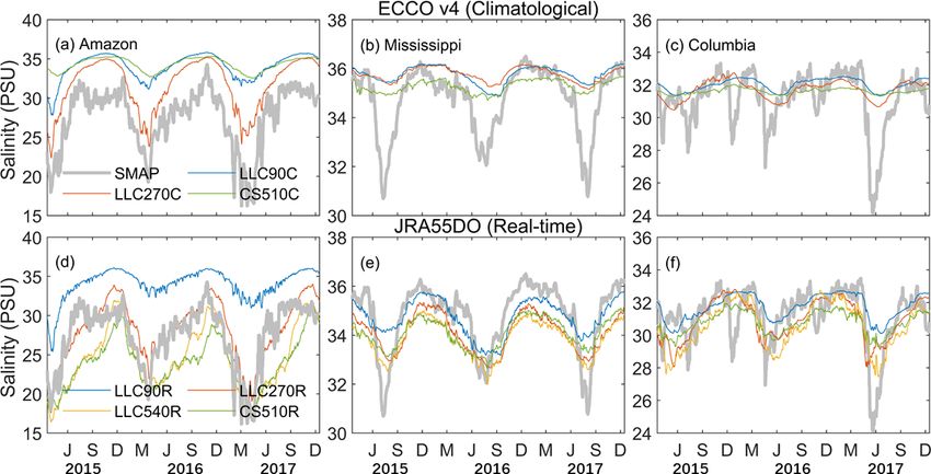
1804 Y. Feng et al.: Improved representation of ECCO river runoff
Table 1. Summary of all experiments. The ECCOv4 and ECCO2 climatological runoff is derived from Fekete et al. (2002) and Stammer et
al. (2004), respectively. A comparison of runoff forcings is shown in Fig. S1.
No. Experiment name Grid type Runoff forcing Grid spacing
1 LLC90C Lat–long–cap ECCOv4 Climatology 55–110 km
2 LLC90R Lat–long–cap JRA55-do 55–110 km
3 LLC270C Lat–long–cap ECCOv4 Climatology 18–36 km
4 LLC270R Lat–long–cap JRA55-do 18–36 km
5 LLC270R_spread Lat–long–cap JRA55-do 18–36 km
6 LLC270R_clim Lat–long–cap JRA55-do 18–36 km
7 LLC540R Lat–long–cap JRA55-do 9–18 km
8 CS510C (Standard ECCO2) Cube–sphere ECCO2 Climatology ∼ 19 km
9 CS510R Cube–sphere JRA55-do ∼ 19 km
The Willmott score is calculated as
n
(Mi − Oi )2
P
i=1
Wskill = 1 − n , (3)
P 2
Mi − Ō + Oi − Ō
i=1
where Mi is the model estimate at ti , Oi is the observation at
time ti , Ō is the mean of the observations, and n is the num-
ber of time records for comparison. Specifically, Wskill = 1
indicates perfect agreement between model and observa-
tions; Wskill = 0 indicates that the model skill is equivalent
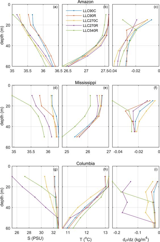
Figure 1. The 10 large rivers (red circles) at 8 coastal regions to the observational mean.
(black boxes) used in our analysis: Amazon and Orinoco (South Furthermore, we conduct our skill assessment for model
America, noted as region 1), Congo (Africa, region 2), Changjiang SSS on multiple experiments across several regions. We also
(Asia, region 3), Ganges and Brahamptura (Asia, region 4), Missis-
use target diagrams (Jolliff et al., 2009) to efficiently visu-
sippi (North America, region 5), Parana (South America, region 6),
Mekong (Asia, region 7), Columbia (North America, region 8). Red
alize a suite of skill metrics. Target diagrams are plotted in
circle size is scaled by the climatological river discharge magnitude. a Cartesian coordinate system with the x axis representing
the unbiased root-mean-square deviation (RMSD); the y axis
represents the bias, and the distance between the origin and
any point within the Cartesian space represents total RMSD.
from 1 April 2015. A total of 10 large rivers at 8 coastal
n
regions spanning from low latitudes to mid-latitudes are se- P
(Mi − Oi )
lected for detailed analysis; these include the Amazon and i=1
Bias = = M̄ − Ō (4)
Orinoco (AZ), Congo (CG), Changjiang (CJ), Ganges and n
Brahamptura (GB), Mississippi (MR), Parana (PA), Mekong
v
u n
uP 2
(MK), and Columbia (CO) rivers (Fig. 1). u Mi − M̄ − Oi − Ō
t i=1
Unbiased RMSD = (5)
2.3 Target diagram and Willmott skill score n
v
u n
uP
The first part of our study compares the simulated salin- u (Mi − Oi )2
t i=1
ity with the synchronized SMAP SSS observations from RMSD = (6)
n
1 April 2015 to 31 December 2017. The level-3 SMAP
version-3 SSS was produced by the Jet Propulsion Labo- M̄ represents the mean of the model estimates. These three
ratory (ftp://podaac-ftp.jpl.nasa.gov, last access: 29 March skill assessment statistics are particularly useful as bias re-
2021; Yueh et al., 2013, 2014). We also compare climato- ports of the size of the model–observation discrepancies.
logical SSS during this period with the World Ocean Atlas Bias values near zero indicate a close match, though it can be
2018 (https://www.nodc.noaa.gov/OC5/woa18/, last access: misleading, as negative and positive discrepancies can can-
29 March 2021). For quantitative comparison, we use the cel each other. The unbiased RMSD removes the mean and
Willmott skill score (Willmott, 1981), a widely used metric is a pure measure of how model variability differs from ob-
for quantifying agreement between models and observations. servational variability. The total RMSD provides an overall
Geosci. Model Dev., 14, 1801–1819, 2021 https://doi.org/10.5194/gmd-14-1801-2021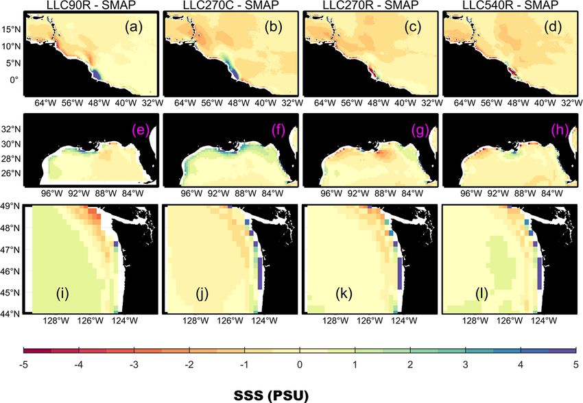
Y. Feng et al.: Improved representation of ECCO river runoff                                                              1805

skill metric, as it includes components for assessing both the   (WOA18). We note that there may be relatively few obser-
mean (bias) and the variability (unbiased RMSD).                 vations incorporated into the objectively analyzed WOA18
   We normalize the bias, unbiased RMSD, and total RMSD          product near the coast, which may over-smooth salinity
by the observational standard deviation (σ0 ) to allow for the   fronts. Additionally, WOA18 is a 55-year climatology from
display of multiple experiment and regional SSS observa-         1955–2010; therefore, we can only compare model climatol-
tions on a single target diagram. According to the defini-       ogy from 2015–2017. Overall, we use SMAP and WOA18
tion of unbiased RMSD, the value should always be positive.      as “observational references”, where our model–observation
However, the X < 0 region of the Cartesian coordinate space      comparisons provide useful information on how SSS changes
may be utilized if the unbiased RMSD is multiplied by the        between experiments rather than determine which experi-
sign of the standard deviation difference (σd ):                 ment is closer to the real world.
                                                                    The upper 10 m SSS biases relative to SMAP, averaged
σd = sign(σm − σo ).                                       (7)   over the 33-month period, for CS510C (standard ECCO2)
                                                                 as well as the LLC540R (highest resolution) are shown in
The resulting target diagram thus provides information about     Fig. S2. Both SMAP and WOA18 have 1/4◦ horizontal grid
whether the model standard deviation is larger (X > 0) or        resolution; therefore, we interpolated all model fields to this
smaller (X < 0) than the observation’s standard deviation, in    grid. For both simulations, negative biases are found from
addition to if the model mean is larger (Y > 0) or smaller       low latitudes to mid-latitudes, while positive biases occur at
(Y < 0) than the observation’s mean.                             high latitudes. When focusing on large river mouth regions
                                                                 (e.g., AZ, PA, and CJ), the SSS bias is reduced in LLC540R.
2.4    Definition of plume characteristics
                                                                 This demonstrates that the choice of runoff forcing impacts
                                                                 SSS at predominantly local scales; however, background cur-
We investigate the role of grid resolution and runoff forcing
                                                                 rents can transport the signal downstream or offshore to the
using several key metrics: plume area, volume, and fresh-
                                                                 open ocean (Liu et al., 2009; Molleri et al., 2010).
water thickness. The plume area is defined as regions with
                                                                    Next, we compute mean model SSS near all selected river
SSS below a given salinity threshold SA (See Sect. 4.2). The
                                                                 mouth regions, along with SMAP and WOA18 (Table 2).
freshwater volume, relative to the reference salinity, S0 , is
                                                                 The corresponding Willmott skill (WS) numbers are listed
defined as the integral of the freshwater fraction:
                                                                 in Table 3. We use the first empirical orthogonal function
                                                                 (EOF) derived from WOA18 to determine river mouth re-
           ZZ Z
                    S0 − S (z)
Vf (SA ) =                      dV ,                       (8)   gions, since WOA18 represents persistent low-salinity zones
                        S0
                  s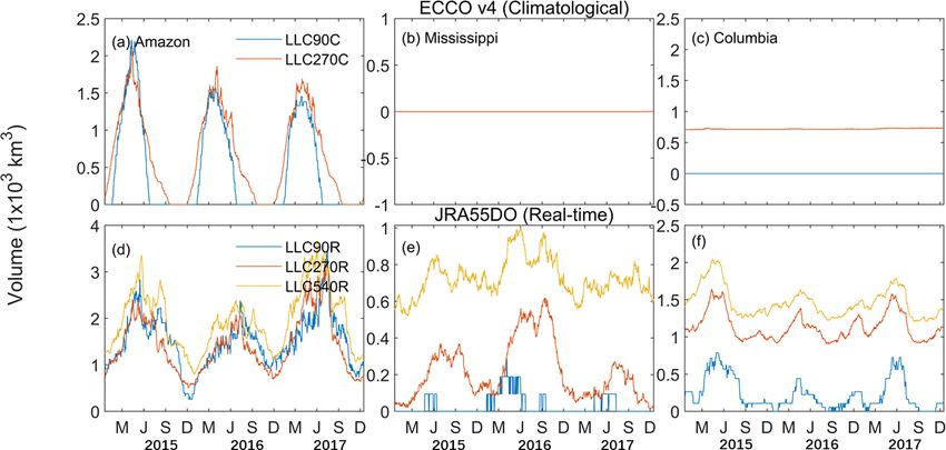
1806                                                            Y. Feng et al.: Improved representation of ECCO river runoff

the daily JRA55DO forcing, the sea surface salinity with the        the SSS and skill scores are comparable between CS510R
point-source forcing (LLC270R) was lower than that with             and LLC540R. Since the model grid type has a negligible
the diffusive forcing (LLC270R_spread). It is possible that         impact on SSS for low-latitude to mid-latitude rivers, we next
decreasing the number of cells adding the freshwater was            focus on discussing model sensitivity to runoff forcing and
equivalent to decreasing the river mouth inlet width, which         model grid resolutions only.
results in the inflow velocity increasing and thus spreads the         To better compare the sensitivity of SSS to river forcing,
riverine water more widely. In contrast, we found the point-        we provide zoomed-in plots of the same comparison shown
source river forcing run using year-by-year JRA55DO and             in Fig. 1 for AZ, MR, and CO Rivers for all LLC simula-
climatological JRA55DO shows a lack of consistency in SSS           tions, representing large, medium, and small rivers (Figs. 2
change compared to the above two cases.                             and S8). The positive bias is greatly reduced when apply-
   A comparison with SMAP shows that Wskill scores be-              ing daily, point-source river forcing, as well as increasing the
come higher when model resolution increases from 1 to               horizontal grid resolution.
1/3◦ (LLC90C vs. LLC270C, LLC90R vs. LLC270R), but                     Time series for all LLC simulations and SMAP, at these
lower when it increases further to 1/6◦ (e.g., LLC270R              three river mouths, are shown in Fig. 3. As in Fig. 2,
vs. LLC540R for Amazon, Ganges/Brahmaputra, Parana).                the bias decreases when daily, point-source river forcing is
The higher or lower Wskill score is consistent with the SSS         used and as the horizontal grid resolution increases. Ad-
decrease. At the AZ region, SSS from LLC270R is less                ditionally, We found the 2017 spring Amazon flood can
than 1 PSU lower than the SMAP average, while that from             be clearly seen when forced by diffusive daily JRA55DO
LLC540R is roughly 3 PSU lower. Therefore, LLC270R re-              (LLC270R_spread), but not in the diffusive climatological
ceives a skill score of 0.92, higher than LLC540R (0.74).           Fekete case (LLC270C). The Mississippi River mouth re-
Although the SSS reduction lowers the model score over-             gion is different from the Amazon in that the annual cycle of
all, we should note that SMAP only has 1/4◦ resolution.             LLC270_spread is stronger than LLC270C. This is because
This means it may not have the capability to resolve those          the seasonality of the Mississippi–Atchafalaya river has been
fine-scale dynamic feathers of the plume compared to high-          oversmoothed in the climatological Fekete. The Columbia
resolution model simulation. In addition, SMAP may under-           river region is consistent with the Amazon in that there is
estimate SSS near the river mouth. Therefore, a larger dis-         an abnormal low salinity in 2017 in LLC270R_spread and
crepancy with SMAP in the high-resolution run does not in-          LLC270R, which is because the peak discharge is success-
dicate that the simulation deviates from the truth.                 fully resolved by JRA55DO.
   The Wskill scores when taking SMAP as the reference                 It is interesting to see the intermediate LLC270 resolu-
show that LLC270R_spread is better than LLC270C for                 tion run is better than the high CS510 resolution run at the
AZ, GB, MR, PA, and CO. This is not surprising since                Amazon region. This is because the Stammer et al. (2004)
the JRA55DO runoff had better temporal resolution than              runoff is smoother spatially and lacks seasonal variability
Fekete runoff. Meanwhile, Wskill scores of LLC270R_spread           compared to the Fekete et al. (2002) runoff in this region
is worse than LLC270R, mainly because of diffusive surface          (Fig. S7). When using DPR forcing, the SSS differences as-
runoff bringing higher SSS than point-source surface runoff         sociated with the river discharge interannual variability can
(Fig. S8).                                                          be resolved as well. For example, the 2017 abnormally low
   When taking the climatological WOA18 as the observa-             SSS near the Amazon river mouth is associated with an ex-
tional reference, experiments forced with the climatological        treme flooding event (Barichivich et al., 2018).
river forcing had a better Wskill score than with real-time forc-      Next, we quantify the difference in mean and variance be-
ing for the Amazon River, but no such pattern for other rivers.     tween the SSS time series of LLC simulations and that of
The lack of consistency is possibly because the simulations         SMAP under daily JRA55DO runoff but using diffusive and
and data are not synchronized in years. A comparison with           point source methods for each (Fig. 4). We found the normal-
the SMAP score shows that most ECCO SSS products had                ized bias with point source is lower than experiments with
comparable skill with SMAP, indicating that they are reliable       diffusive source. The normalized unbiased RMSD decrease
to use at the climatological mean level.                            is ignorable compared to the normalized bias decrease. This
   The higher or lower Wskill score is consistent with how          means the total normalized RMSD improvements are primar-
much the model deviates from the observational reference.           ily due to the normalized bias decrease. We find that most
At the AZ region, SSS from LLC270R is less than 1 PSU               unbiased RMSD remains negative when varying the runoff
lower than the SMAP average, while LLC540R is roughly               forcing from climatological to daily. This implies that the
3 PSU lower. Therefore, LLC270R receives a skill score              variance of LLC simulations remains lower than SMAP ob-
0.92, higher than LLC540R (0.74). This also occurs with             servations as the runoff forcing changes. The only exception
LLC270C and LLC270R when using WOA18 as the refer-                  is the Congo river, which is a near-Equator eastern boundary
ence.                                                               plume that freshwater transport may distinguish from others
   For rivers in tropical and temperate zones, the CS510 grid       (Palma and Matano, 2017).
has a resolution comparable with the LLC540 grid; therefore,

Geosci. Model Dev., 14, 1801–1819, 2021                                             https://doi.org/10.5194/gmd-14-1801-2021
Y. Feng et al.: Improved representation of ECCO river runoff 1807
Table 2. The SSS near river mouth for WOA18, SMAP, and all experiments for the selected regions.
River Abb. Discharge WOA SMAP LLC LLC LLC LLC LLC LLC LLC CS CS
mouth (m3 /yr) 18 90C 90R 270C 270R_spread 270R 270R_clim 540R 510C 510R
Amazon/Orinoco AZ 6440 32.7 27.5 34.0 34.1 31.7 30.4 28.2 27.6 24.6 34.3 23.8
Congo CG 1270 33.6 33.7 34.7 34.3 34.6 35.3 33.9 35.2 33.7 34.9 34.1
Changjiang CJ 907 32.9 31.4 33.1 32.8 33.0 32.2 32.2 32.4 31.8 32.5 30.9
Ganges/Brahamptura GB 643 29.3 27.5 30.9 29.4 29.5 27.6 27.2 27.1 23.9 29.7 25.6
Mississippi MR 552 33.5 34.8 35.8 34.7 35.8 34.4 34.1 33.3 33.8 35.3 34.1
Parana PA 517 28.9 27.3 33.7 31.0 31.1 24.9 24.7 25.5 20.0 33.8 20.0
Mekong MK 504 32.9 32.9 33.5 32.6 32.3 31.2 30.3 29.8 31.0 31.8 28.5
Columbia CO 167 30.7 31.0 32.0 31.7 31.7 31.3 30.8 30.5 30.3 31.4 30.4
Table 3. The Willmott skill score for each run as compared with WOA18 and SMAP. The river mouth was recognized by the first EOF
of WOA18 (see Figs. 5 and S1). Note that WOA18 data are a 30-year climatology (1981–2010) and not in the same period as SMAP and
experiments.
River SMAP LLC90C LLC90R LLC270C LLC270R_spread LLC270R LLC270R_clim LLC540R CS CS
mouth 510C 510R
with SMAP
Amazon/Orinoco – 0.50 0.50 0.71 0.83 0.92 0.92 0.79 0.46 0.73
Congo – 0.58 0.64 0.69 0.46 0.89 0.47 0.88 0.60 0.87
Changjiang – 0.53 0.59 0.51 0.30 0.64 0.31 0.83 0.59 0.85
Ganges/Brahamptura 0.61 0.71 0.69 0.83 0.85 0.84 0.69 0.57 0.70
Mississippi 0.55 0.79 0.53 0.75 0.77 0.69 0.75 0.49 0.72
Parana 0.37 0.51 0.45 0.60 0.62 0.56 0.40 0.37 0.40
Mekong 0.79 0.90 0.77 0.67 0.54 0.47 0.63 0.74 0.38
Columbia 0.46 0.60 0.49 0.68 0.73 0.70 0.74 0.27 0.61
with WOA
Amazon/Orinoco 0.47 0.73 0.69 0.87 0.62 0.64 0.78 0.47 0.54 0.44
Congo 0.54 0.60 0.67 0.70 0.48 0.94 0.47 0.95 0.64 0.92
Changjiang 0.44 0.82 0.94 0.68 0.70 0.70 0.73 0.72 0.78 0.54
Ganges/Brahamptura 0.73 0.72 0.90 0.92 0.77 0.78 0.82 0.51 0.73 0.59
Mississippi 0.69 0.46 0.59 0.46 0.76 0.68 0.60 0.73 0.49 0.66
Parana 0.87 0.40 0.45 0.45 0.42 0.42 0.42 0.29 0.40 0.29
Mekong 0.64 0.84 0.87 0.83 0.39 0.45 0.59 0.54 0.71 0.30
Columbia 0.47 0.51 0.62 0.63 0.85 0.87 0.82 0.84 0.51 0.90
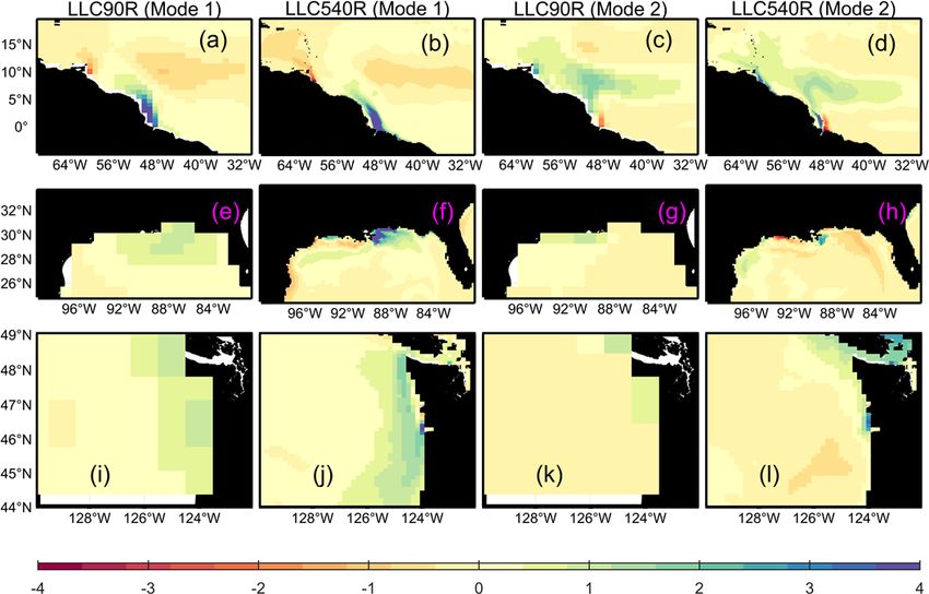
We also examine the bias and variance on the target dia- 4 Impact on river plume properties
gram for experiments with varying grid resolution but sim-
ilar daily runoff forcing (Fig. 5). Our results show that the 4.1 EOF analysis of SSS
normalized bias decreases as the model resolution increases,
which is consistent with the SSS reduction in Table 2 and rel- We next investigate how model runoff improvements impact
atively low Wskill in Table 3. The unbiased RMSD decreases river plume properties such as plume area, volume, and fresh-
slightly with the sign remaining negative as the model reso- water thickness, since we are interested in how the widely
lution increases. This occurs everywhere, except for the two used general ECCOv4 (forced by Fekete runoff)) will be dif-
largest rivers (AZ and CG) where the sign becomes positive ferent from the new DPR implementation. We limited our
for LLC540R, indicating that the model variance exceeds the next discussion to LLC#C/R cases only (experiments 1, 2, 3,
SMAP variance when using the high-resolution grid. In sum- 4, and 7). We first evaluate the plume SSS signature and dy-
mary, the comparison with synchronized SMAP shows that namics through EOFs; the mean is removed before the EOF
using daily runoff and finer horizontal grid resolution im- analysis. The first and second mode of AZ, MR, and CO us-
proves the representation of SSS variability but at a cost of ing the same grid resolution but different runoff forcing is
increased SSS bias. shown in Figs. 6 and S4. The spatial pattern reveals the salin-
ity anomaly caused by the runoff, while the PC time series
shows the timing. A single value in spatial pattern or PC
time series does not have a clear physical meaning, but to-
gether they reveal how much salinity deviates from the mean.
https://doi.org/10.5194/gmd-14-1801-2021 Geosci. Model Dev., 14, 1801–1819, 2021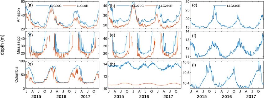
1808                                                                Y. Feng et al.: Improved representation of ECCO river runoff

Figure 2. Zoomed-in view of SSS difference between model experiments and SMAP observations for large (Amazon, a–d), medium (Mis-
sissippi, e–h), and small (Columbia, i–l) rivers.

Figure 3. Areally averaged SSS in the Amazon, Mississippi, and Columbia river mouth regions (see Fig. S3) with climatological diffusive
and daily, point-source runoff forcing for SMAP (thick gray line) and experiments (thin colored lines) with varying horizontal grid resolution.
The method used to characterize the river mouth region is described in Sect. 3.

The PC time series for experiments with DPR forcing clearly               LLC270R (LLC270C). The spatial pattern reveals the pres-
shows similar seasonal cycles, albeit with larger amplitudes              ence of a low-salinity tongue; this is located in a narrow band
and interannual variability.                                              along the northeastern South American coast from February–
   For the AZ region, the LLC270R and LLC270C spa-                        June, which is associated with the large river discharge and
tial patterns are similar for the first and second mode. The              the northward-flowing Brazil Current. The second mode of
first mode accounts for 59 % (72 %) of the total variance in              LLC270R (LLC270C) accounts for 33 % (23 %) of the total

Geosci. Model Dev., 14, 1801–1819, 2021                                                     https://doi.org/10.5194/gmd-14-1801-2021
Y. Feng et al.: Improved representation of ECCO river runoff                                                               1809

Figure 4. SSS target diagram near the selected river mouths (see
Fig. S3) for LLC270R_spread and LLC270R simulations.

variance. The spatial pattern shows that the plume-like fea-
                                                                    Figure 5. Same as Fig. 4, but for LLC90R, LLC270R, and
tures extend northwestward to the Caribbean Sea and Central
                                                                    LLC540R.
Equatorial Atlantic Ocean from May–September. This pat-
tern is driven by Ekman currents associated with northeast-
erly wind stress, and the transport to the Central Equator is       the plume offshore, where it is influenced by the California
due to the North Equatorial Counter Current (NECC; Lentz            Current over long timescales and subsequently veers south-
1995a, b).                                                          ward and offshore (Banas et al., 2009). This seasonal pattern
   For the MR region, the first and second mode of LLC270R          is shown in the first LLC270R mode and second LLC270C
(LLC270C) explains 53 % (66 %) and 29 % (18 %) of the to-           mode.
tal variance, respectively. The spatial pattern of the first mode      The first and second EOF modes for AZ, MR, and CO with
is generally similar. There is a bulge-like plume feature that      daily runoff forcing in coarse (LLC90R) and fine (LLC540R)
occupies a region near the MR mouth with a southeast ex-            grid resolution are shown in Figs. 7 and S5. The plume-
tension to the central Gulf of Mexico from May–October              like features and associated dynamics are similar to LLC270
(Fig. S4), while the freshwater signal in the vicinity of the       in both runs. Additionally, the higher-resolution LLC540R
southeast MR mouth is stronger in LLC270R. The extension            resolves fine-scale plume structure for a number of ma-
of low-salinity waters is due to the upwelling of favorable         jor rivers, which was previously revealed by satellite ob-
winds (southwesterly) from late spring to summer, which             servations, regional simulations, or neural network methods
transport the MR freshwater offshore (Walker, 1996).                (e.g., meanders and rings of the AZ plume due to the NBC
   The first and second mode explains 63 % (56 %) and 29 %          retroflection; Molleri et al., 2010); “horseshoe” patterns of
(33 %) of the variability at the CO region in LLC270C               the MR plume associated with Texas floods (Fournier et al.,
(LLC270R), respectively. It has been previously recognized          2016b); and the bidirectional CO plume during variable sum-
that the CO plume exhibits seasonal variability forced by           mer wind patterns (Liu et al., 2009). Overall, EOF SSS anal-
wind and freshwater discharge (García Berdeal et al., 2002).        ysis shows that general plume pattern and dynamics are grid
During winter, Ekman transport resulting from the northward         independent; however, fine-scale plume structures are only
winds constrains the plume against the Washington coast.            resolved by high-resolution simulations.
Downwelling-favorable wind stresses strengthen the anti-
cyclonic rotation of the river plume, resulting in a coastally
attached winter plume. In contrast, prevailing southward
wind stress results in offshore Ekman transport; this advects

https://doi.org/10.5194/gmd-14-1801-2021                                             Geosci. Model Dev., 14, 1801–1819, 2021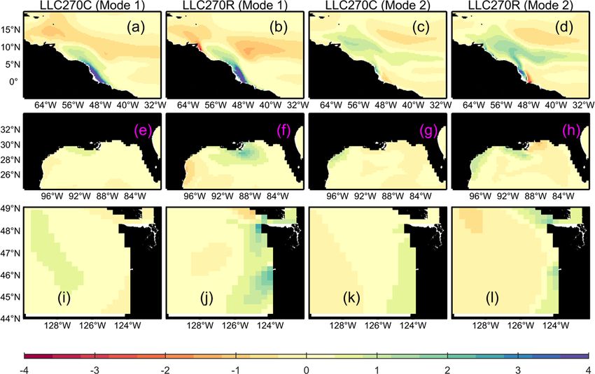
1810 Y. Feng et al.: Improved representation of ECCO river runoff
Figure 6. First and second EOF spatial patterns from the LLC270C and LLC270R simulations for the Amazon, Mississippi, and Columbia
rivers. The corresponding PC time series are normalized by the standard deviation and multiplied back to the spatial mode.
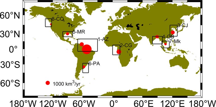
4.2 Plume area, volume, and freshwater thickness LLC90R, LLC270R, and LLC540R, respectively. The fresh-
water volume in coarse-, intermediate-, and high-resolution
We first calculated the plume area using a salinity thresh- runs is comparable, with values of ∼ 1.5–2 × 10² km3 . The
old from 28 to 36 PSU. The 3-year-average plume area for plume area and volume in the MR region is more sensi-
AZ, MR, and CO river region for different LLC configu- tive to the model grid resolution than AZ and CO. The
rations are present in Fig. 8. Under either the climatologi- LLC540R plume area is∼ 3–4 times higher than LLC270R,
cal diffusive or DPR river forcing, we could clearly see the while LLC270R is ∼ 6–7 times higher than LLC90R. For
plume area increase when model resolution increased from the CO region, the plume area when using DPR forcing
1◦ to 1/3◦ for all regions. However, when model resolu- is similar between intermediate- and fine-resolution exper-
tion was increased to 1/6◦ , the plume area further increase iments, with the area in LLC270R and LLC540R increas-
can only be clearly seen in the Mississippi River region. To ing to ∼ 1 × 10⁵ km2 during the 2015 flood year. In con-
highlight the seasonal and interannual variability at the given trast, LLC540R maintains a larger plume volume than the
threshold, we also show the plume area and volume within intermediate-resolution run.
SA = 30 PSU under the climatological and daily runoff forc- The sensitivity of plume area and volume to runoff forcing
ing at the coarse, intermediate, and high-resolution runs and grid resolution reflects the experiment’s ability to resolve
(Figs. S6, 9). Figure 9 presents a time series of freshwater the horizontal advection and downward mixing of riverine
volume within the given salinity during this period. There is a freshwater. This can be partially reflected in the freshwa-
stronger interannual variability when using DPR, along with ter thickness calculation, which is shown in Fig. 10. For the
larger plume area and volume during flood years. The MR intermediate-resolution experiments, the maximum freshwa-
and CO plume area and volume cannot be explicitly resolved ter thickness δfw is over 10, 5, and 4 m near the AZ, MR,
at the SA = 30 threshold when using the climatological and and CO river mouths when using DPR, as opposed to 4,
runoff forcing since river runoff has been distributed over 2, and 2 m when using climatological runoff. Additionally,
broad spatial grids and surface salinity decrease is small. For the freshwater thickness in experiments with DPR but dif-
the AZ region, the averaged plume area (volume) approaches ferent grid resolutions (LLC270R and LLC540R) demon-
6 × 10⁴ km2 (7 × 10² km3 ) in LLC270C, whereas it is only strates that a coherent plume rotates and responds to exter-
about 3 × 10⁴ km2 (5 × 10² km3 ) in LLC90C. In contrast, nal wind and background flows; this coastal plume struc-
the MR and CO plume area (volume) is easily recognized ture is largely absent in the coarser LLC90R. The coarse-
when using DPR forcing. The AZ plume increases as the grid resolution experiment exhibits a more diffuse response, with
resolution increases, reaching 10, 13, and 17 × 104 km2 in low salinity near MR and CO river mouths. Note that the
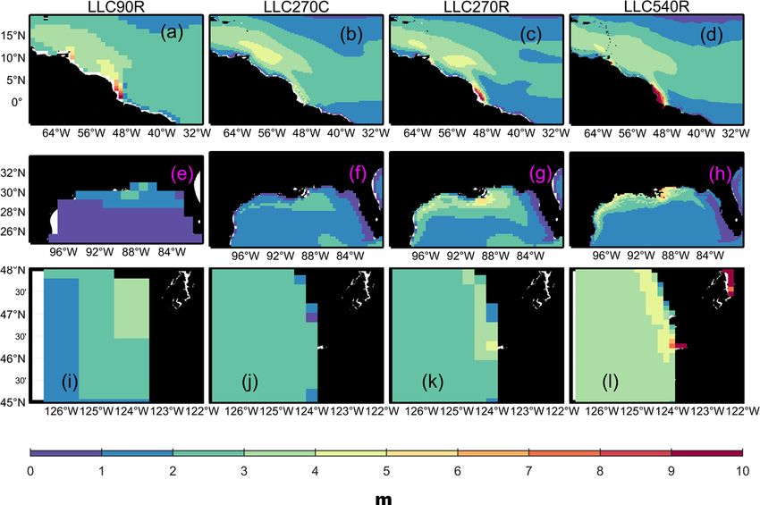
Geosci. Model Dev., 14, 1801–1819, 2021 https://doi.org/10.5194/gmd-14-1801-2021Y. Feng et al.: Improved representation of ECCO river runoff 1811 Figure 7. Same as Fig. 6 but for the LLC90R and LLC540R simulations. The corresponding PC time series are normalized by the standard deviation and multiplied back to the spatial mode shown in Fig. S5. Figure 8. 2015–2017 averaged plume area at salinity threshold SA from 28 to 36 for the Amazon, Mississippi, and Columbia River regions. runoff forcing is identical between LLC90R, LLC270R, and compared to the northern Brazilian shelf (AZ) and Washing- LLC540R experiments, and differences in plume area, vol- ton shelf (CO). When adding the same amount of freshwater ume, and freshwater thickness are due to model resolution in shallow water regions, high-resolution experiments gen- alone. The freshwater flux in the higher resolution experi- erate a larger pressure gradient force than the intermediate ments can result in larger inflow velocities, a stronger baro- resolution, which drive a stronger baroclinic effect and el- clinic response, and consequently a more vigorous coastal evate coastal currents. The alongshore currents can advect plume. The plume area and volume in the MR region is the MR Plume water downcoast, enlarging the plume area. more sensitive to grid resolution – this possibly results from Besides, the plume waters may be entrained downward by the representation of shelf bathymetry. The Texas–Louisiana strong sub-grid vertical mixing and adjustment, e.g., meso- shelf is wider and shoals more gradually from the coastline scale eddies, when flowing offshore to the open ocean as https://doi.org/10.5194/gmd-14-1801-2021 Geosci. Model Dev., 14, 1801–1819, 2021
1812                                                           Y. Feng et al.: Improved representation of ECCO river runoff

Figure 9. Freshwater volume within 30 PSU for the Amazon, Mississippi, and Columbia river regions for various experiments; reference
salinity is 36 PSU.

the horizontal resolution increases from intermediate to high.      reflecting that heat is preserved at the surface due to the in-
The eddies in the high-resolution run at AZ and CR may              crease in subsurface stratification.
break up the plumes, shrinking the area compared to the low-           The sensitivity of stratification in the above analysis im-
to-intermediate-resolution run (Fig. S6).                           plies that the MLD can be altered by river forcing and grid
                                                                    resolution. We compare the MLD in the vicinity of AZ, MR,
                                                                    and CO during the simulation period in Fig. 12. The MLD in
4.3    Impact on ocean properties associated with SSS               our calculation uses the threshold method, in which deeper
                                                                    levels are examined until one is found with density differing
                                                                    from that the near surface by more than 0.03 kg/m3 (de Boyer
In this section, we examine the sensitivity of stratification
                                                                    Montégut et al., 2004). This reflects the maximum depth
and mixed layer depth (MLD) between different experi-
                                                                    of the boundary layer that is sustained by riverine freshwa-
ments. Figure 11 shows 3-year averaged vertical profiles of
                                                                    ter. Interestingly, all experiments simulate the annual cycle
salinity, temperature, and vertical density gradient dρ/dz (ρ
                                                                    of MLD. There was relatively shallow MLD from April to
is the potential density) near the AZ (a–c), MR (d–f), and
                                                                    December, which corresponds to periods of high river dis-
CO (g–i) river mouths, respectively. The profiles are aver-
                                                                    charge. The MLD in the DPR forcing and high-resolution
aged over the horizontal regions shown in Fig. S3. The ver-
                                                                    scenario is shallower than the climatological, low-resolution
tical density gradient is an important indicator of stratifica-
                                                                    scenario, which is consistent with vertical salinity and strati-
tion strength. The salinity differences between climatologi-
                                                                    fication profiles shown in Fig. 11.
cal (LLC90/270C) and DPR forcing (LLC90/270R) are large
near the surface and diminish with increasing depth. The
temperature difference when using the two types of runoff
forcing is insignificant, demonstrating that the stratification     5   Discussion and conclusions
is primarily determined by salinity and the addition of fresh-
water. Additionally, DPR forcing greatly increases subsur-          In this study, we investigate the model sensitivity of runoff
face stratification, which implies a decrease in vertical mix-      forcing and grid resolution and type under the ECCO frame-
ing.                                                                work. We find that DPR greatly improves model representa-
   Figure 11 also shows sensitivity of upper-ocean stratifi-        tion of global rivers, with horizontal model resolution having
cation to various model grid resolutions. The profiles show a       a substantial control on SSS in the vicinity of river mouths.
significant decrease in salinity from the surface to 50 m depth     We observe no major changes in tropical and temperate river
as the resolution increases, which impacts the stratification       mouth SSS when using cube–sphere or LLC grid types when
(panels c, f, and i). We note that the vertical density gradient    using the same river forcing. A comparison with synchro-
has a subsurface maximum in the coarse- and intermediate-           nized SMAP observations shows that the use of DPR forcing
resolution run, while the high-resolution experiment has a          and intermediate grid resolution can increase the model per-
surface maximum due to low-salinity water concentrated in           formance in simulating SSS in the vicinity of river mouths.
the surface level. SST is highest in LL540R at AZ and MR,           However, further increasing model grid resolution from inter-

Geosci. Model Dev., 14, 1801–1819, 2021                                              https://doi.org/10.5194/gmd-14-1801-2021
Y. Feng et al.: Improved representation of ECCO river runoff 1813 Figure 10. Freshwater thickness for the Amazon, Mississippi, and Columbia river regions in LLC90R, LLC270C, LLC270R, and LLC540R experiments. mediate to high may result in an additional SSS bias towards creasing the model grid resolution from coarse to intermedi- fresher values. ate increases the river plume area and volume, while further Previous theoretical modeling studies have demonstrated increasing the model resolution from intermediate to high has that, in the absence of external forcing, large river plumes in- mostly regional effects. Shallow and wide shelf regions, such fluenced by rotational effects tend to veer anticyclonically as the Mississippi Delta, are more sensitive compared to AZ and form a bulge region near the river mouth as well as and CO. Nowadays, the increased computational power al- an along-shore downstream coastal current as Kelvin waves lows GODAS products such as ECCO to provide data at dif- (Kourafalou et al., 1996; Yankovsky and Chapman, 1997). ferent resolutions, which supports regional scientific studies Additionally, idealized numerical simulations have revealed using a data analytical approach or offline method (e.g., the that river plume behavior is greatly impacted by external Lagrangian method; Meng et al., 2020; Liang et al., 2019). forcing. Chao (1988a, b) demonstrated that vertical mix- Our results suggest that how high-resolution products should ing, bottom drag, and bottom slope greatly impact the spin- be used depending on the spatiotemporal dynamics as well up, maintenance, and dissipation of river plumes. Fong and as geomorphology characteristic of the studied region itself. Geyer (2001) revealed that a surface-trapped river plume We also found that using DPR forcing and increasing would thin and be advected offshore by cross-shore Ekman the model grid resolution can stabilize the water column transport. Fong and Geyer (2002) suggested that the ambi- at the subsurface and shoal the MLD. This may have sig- ent current, which is in the same direction as the geostrophic nificant implications for biogeochemical cycles and air–sea coastal current, can augment plume transport. Our ECCO exchange in coastal zones. From the biogeochemistry per- experiments are examining the above river plume dynamic spective, freshwater introduced by the river increase shelf theory globally with realistic topography and external atmo- stratification, preventing the reoxygenation of bottom wa- spheric forcing. Our EOF analysis of SSS at the AZ, MR, and ters and thus may generate large hypoxic regions (Fennel CO shelves show that the general spatial and temporal pat- et al., 2013; Feng et al., 2019). From the air–sea interac- terns plume related to river discharge, wind, and currents are tion perspective, on one hand, SST can trigger deep atmo- independent of the grid resolutions and forcing formulations spheric convection and strong rainfall. On the other hand, examined in this study, which are quite consistent with those strong near-surface stratification may inhibit cooling and in- previous studies. However, higher resolution and DPR forc- tensify tropical cyclones (Cione and Uhlhorn, 2003; Neetu et ing may be particularly important for resolving the fine-scale al., 2012; Rao and Sivakumar, 2003; Sengupta et al., 2008; plume dynamics for small rivers. Using DPR forcing and in- Vialard and Delecluse, 1998; Vinaychandran et al., 2002). https://doi.org/10.5194/gmd-14-1801-2021 Geosci. Model Dev., 14, 1801–1819, 2021
1814                                                          Y. Feng et al.: Improved representation of ECCO river runoff

                                                                     The present state-of-the-art regional-scale estuarine mod-
                                                                  els can simulate estuarine hydrodynamics and biogeochemi-
                                                                  cal processes in a robust manner. The inlet approach, which
                                                                  defines a rectangular breach in coastal land cells with uni-
                                                                  form density and discharge, is widely used (Herzfeld, 2015;
                                                                  Garvine, 2001). An additional barotropic pressure term may
                                                                  be added to account for pressure gradients induced by the
                                                                  freshwater plume (Schiller and Kourafalou, 2011). The inlet
                                                                  approach has also been used in global z-coordinate models
                                                                  by injecting freshwater in multiple vertical grid cells (Griffies
                                                                  et al., 2005). In our simulations, changes in sea level are re-
                                                                  distributed over all vertical grid cells by the rescaled height
                                                                  vertical coordinate. This is similar to the inlet approach in
                                                                  the regional models, which add a mass or volume flux of
                                                                  freshwater to a breach in coastal land cells (Garvine, 1999).
                                                                  Herzfeld (2015) investigated the role of model resolution
                                                                  on plume response at the Great Barrier Reef (GBR) using
                                                                  the Regional Ocean Modeling System (ROMS). The study
                                                                  found that the plume veered left and followed a northward
                                                                  trajectory to Cape Bowling Green in a 1 km resolution model
                                                                  but not in a 4 km resolution model. Our findings are consis-
                                                                  tent with this result; plume properties in our intermediate-
                                                                  resolution simulations are more clearly detected than in the
                                                                  coarse-resolution simulations. In addition, our results expand
                                                                  on their findings by showing that the sensitivity of plume
                                                                  properties in high-resolution models are highly dependent
                                                                  on shelf bathymetry. Schiller and Kourafalou (2010) inves-
                                                                  tigated the dynamics of large-scale river plumes in idealized
                                                                  numerical experiments using HYCOM to address how the
                                                                  development and structure of a buoyant plume is affected by
                                                                  the vertical and horizontal redistribution of river inflow and
Figure 11. Mean 3-year (2015–2017) salinity, potential tempera-
                                                                  bottom topography. Their experiments show that a narrow
ture, and vertical density gradient (dρ/dz) profiles.             inlet and flat bottom facilitate a larger right-turning plume
                                                                  bulge region compared to a wide inlet and sloped bottom
                                                                  (see their Fig. 8; Riv2c-f, Riv2c-s). This is complementary
We envision that future work investigating river impacts on       to our findings that the MR plume, located on the wide and
ocean–atmosphere and Earth system dynamics could be ac-           shallow LA shelf, has a larger horizontal plume area com-
complished by coupling our improved ECCO simulations              pared to the AZ and CO plume when increasing the hori-
with an atmospheric general circulation model (AGCM).             zontal resolution from intermediate to high. However, their
   In the state-of-the-art OGCMs, ESMs, and most GODAS            discussion was limited to an idealized, rectangular model do-
products, river runoff is incorporated into coarse-resolution     main without external forcing, while our model simulations
grids as augmented precipitation. Climatological runoff forc-     provide a realistic application to natural river plume systems.
ing is often used in conjunction with artificial spreading,       The global application of the regional inlet representation of
along with a virtual salt flux scheme. Tseng et al. (2016) ex-    river forcing was also used by NOAA’s Geophysical Fluid
amined model sensitivity to the spreading radius, turbulent       Dynamics Laboratory (GFDL) models (Griffies et al., 2005).
mixing parameterization, reference salinity, and vertical dis-    An internal, pre-computed salinity source term was intro-
tribution of riverine freshwater on 1◦ resolution in the Com-     duced into multiple vertical layers. However, river represen-
munity Earth System Model (CESM). For all factors exam-           tation was done through VSF rather than through real mass
ined, they found that the model results are most sensitive to     or freshwater volume flux. Adding the real volume and mass
the spreading radius, which substantiates the importance of       of freshwater through multiple layers has been widely used
our finding that the associated plume properties, including       in regional models like ROMS; it may be useful to adapt this
the area and hence the SSS near river mouths, exhibit strong      technology into future ECCO simulations and compare the
responses when switching the runoff flux from diffusive cli-      results with the current surface injection methods.
matological to daily point source.                                   For the global ocean, river runoff is much smaller than
                                                                  the precipitation and evaporation flux; therefore, for most

Geosci. Model Dev., 14, 1801–1819, 2021                                            https://doi.org/10.5194/gmd-14-1801-2021
Y. Feng et al.: Improved representation of ECCO river runoff 1815
Figure 12. 2015–2017 daily MLD, averaged in the vicinity of the Amazon River (a, b, c), Mississippi River (d, e, f), and Columbia River (g,
h, i) mouth. MLD is computed based on de Boyer Montegut et al. (2004).
OGCMs, ESMs, and GODAS products it is parameterized. state estimates (ECCO-Darwin, Carroll et al., 2020) will help
One of the most significant expected signatures of global better resolve the global carbon budget (Friedlingstein et al.,
warming is an acceleration of the terrestrial hydrological cy- 2019).
cle (IPCC, 2021; Piecuch and Wadehra, 2020). Both can sig- LOAC development has historically had a low priority
nificantly affect the magnitude, distribution, and timing of in OGCMs, ESMs, and GODAPs and exchange of fresh-
global runoff, leading to extremes in the frequency and mag- water between rivers/estuaries and the coastal ocean has
nitude of floods and droughts. When considering issues re- been previously neglected. Our results demonstrate that the
lated to water resource management under climate and land representation of runoff forcing in ECCO simulations is
use and land cover change, a key question such as “how will a major source of bias for coastal SSS. We believed our
coastal oceans be impacted from flood and drought events?” improvements of river runoff in ECCO will directly con-
is challenging to answer (Fournier et al., 2019). In the future, tribute to (i) the evaluation, understanding, and improvement
high-resolution global-ocean circulation models with DPR of river-dominated coastal margins in global-ocean circu-
forcing may help identify the primary forcing mechanisms lation models; (ii) investigation of mechanisms that drive
(such as those from climate-driven extreme events) that drive seasonal and interannual variability in coastal plume pro-
spatiotemporal variability of large river plume systems just cesses; and (iii) bridging the gap between land–ocean inter-
as skillfully as regional model setups. actions. These efforts will ultimately help to better resolve
Improved model representation of rivers may not be as im- land–ocean–atmosphere processes and feedbacks in next-
portant for global- or basin-scale hydrological cycles as pre- generation Earth system models.
cipitation and evaporation (Du and Zhang, 2015) but may
be critical for the global carbon cycle (Friedlingstein et al.,
2019; Resplandy et al., 2018). River delivers large amounts Code and data availability. The MITgcm and user manual
of anthropogenic nutrients to the coastal zone (Seitzinger et are available from the project website: http://mitgcm.org/
al., 2005, 2010). The autochthonous production will trans- (last access: 29 March 2021). The ECCOv4 setup can be
form inorganic nutrients to organic nutrients while seques- found at http://wwwcvs.mitgcm.org/viewvc/MITgcm/MITgcm_
contrib/llc_hires/ (Menemenlis, 2020a). The exact version
tering atmospheric CO2 . More importantly, rivers also de-
of MITgcm, ECCOv4 configuration, and MATLAB routines
liver dissolved organic carbon (DOC) and particulate or- to process the ECCOv4 output, generate the target model
ganic carbon (POC) to the coastal ocean, which can be rem- skill assessment diagram, and produce the paper figures are
ineralized and released as CO2 to the atmosphere. Until re- archived on Zenodo (https://doi.org/10.5281/zenodo.4106405,
cently, most global-ocean biogeochemistry models omitted Feng, 2020). The SMAP observations can be downloaded
or poorly represented riverine point sources of nutrients and from http://apdrc.soest.hawaii.edu/las/v6/dataset?catitem=2928
carbon. Lacroix et al. (2020) added yearly-constant riverine (Menemenlis, 2020b). The model forcing and simulated salin-
loads to the ocean surface layer on coarse-resolution (1.5◦ ) ity fields at different resolutions are archived on Zenodo
models and assessed that CO2 outgassing from river loads (https://doi.org/10.5281/zenodo.4095613, Zhang, 2020).
accounted for ∼ 10 % of the global ocean CO2 sink. We an-
ticipate that the implementation of DPR forcing and higher-
resolution grids in ESMs and the ECCO biogeochemical
https://doi.org/10.5194/gmd-14-1801-2021 Geosci. Model Dev., 14, 1801–1819, 2021You can also read