Journal of Computational Physics - Purdue Engineering
←
→
Page content transcription
If your browser does not render page correctly, please read the page content below
Journal of Computational Physics 459 (2022) 111139

                                                           Contents lists available at ScienceDirect

                                               Journal of Computational Physics
                                                                   www.elsevier.com/locate/jcp

A unified Quasi-Spectral Viscosity (QSV) approach to shock
capturing and large-eddy simulation
Victor C. B. Sousa a,∗ , Carlo Scalo a,b
a
    School of Mechanical Engineering, Purdue University, West Lafayette, IN, 47907, United States of America
b
    School of Aeronautics and Astronautics, Purdue University, West Lafayette, IN, 47907, United States of America

a r t i c l e             i n f o                          a b s t r a c t

Article history:                                           The Quasi-Spectral Viscosity (QSV) method is a novel closure for a high-order finite-
Received 23 March 2021                                     difference discretization of the filtered compressible Navier-Stokes equations capable of
Received in revised form 11 February 2022                  unifying dynamic subfilter scale (SFS) modeling and shock capturing under a single
Accepted 6 March 2022
                                                           mathematical framework. Its innovation lies in the introduction of a physical-space
Available online 16 March 2022
                                                           implementation of a spectral-like SFS dissipation term by leveraging residuals of filter
Keywords:                                                  operations, achieving two goals: (1) estimating the energy of the resolved solution near
Shock capturing                                            the grid cutoff; (2) imposing a plateau-cusp shape to the spectral distribution of the
Large-Eddy Simulation                                      added dissipation. The QSV approach has been tested in a variety of flows to showcase
Spectral Viscosity                                         its capability to act interchangeably as: a shock capturing method, in the Shu-Osher,
                                                           shock/vortex or shock/wall interactions problems; or as a SFS closure, in subsonic Taylor
                                                           Green Vortex (TGV), and supersonic/hypersonic turbulent channel flows. QSV performs
                                                           well compared to previous eddy-viscosity closures and shock capturing methods in such
                                                           test cases. In a supersonic TGV flow, a case which exhibits shock/turbulence interactions,
                                                           QSV alone outperforms the simple superposition of separate numerical treatments for SFS
                                                           turbulence and shocks. QSV’s combined capability of simulating shocks and turbulence
                                                           independently, as well as simultaneously, effectively achieves the unification of shock
                                                           capturing and Large-Eddy Simulation.
                                                                                                             © 2022 Elsevier Inc. All rights reserved.

1. Introduction

   Modeling approaches for hydrodynamic turbulence and shock formation have taken historically different paths, despite
both phenomena being characterized by an energy cascade from large to small scales due to nonlinear interactions [13,15].
This suggests that the modeling approach for such distinct phenomena could be indeed unified, allowing accurate and
numerically stable results of highly compressible turbulent flows on relatively coarse grids with a single artificial-dissipation
approach. An application that benefits from such development is the modeling of transitional or fully turbulent hypersonic
boundary layers characterized by steep, shock-like, flow gradients that can arise as a result of both nonlinear waves or
hydrodynamics.
   The Large-Eddy Simulation (LES) methodology was developed to relax the Reynolds number constraint on numerical
simulations of hydrodynamic turbulence. In an LES, the original Navier-Stokes equations are filtered via a low-pass band
filtering operation which commutes with the spatial and temporal derivatives in an attempt to separate the large, or filtered,

    *   Corresponding author.
        E-mail address: vsousa@purdue.edu (V. C. B. Sousa).

https://doi.org/10.1016/j.jcp.2022.111139
0021-9991/© 2022 Elsevier Inc. All rights reserved.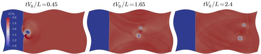
V. C. B. Sousa and C. Scalo                                                             Journal of Computational Physics 459 (2022) 111139

scales from the small, subfilter scales (SFS). Although such an operation is able to seamlessly separate the scales when
applied to linear terms, when it acts upon nonlinear components, an unclosed term, connected to energy flux between
scales, appears. The genesis of such a term is connected to the dynamics of large and smalls scales being coupled. Ultimately,
the LES method directly computes the evolution of the large scales by modeling the energy flow towards the small scales
via a dissipative term.
    The effort spent in the development of subfilter-models for LES has been considerable and it was initially focused on
incompressible flows. Most of these models are of the eddy-viscosity type, where the energy flux to the small scales is
modeled as a viscous dissipation process within a fluid. In such models, the fluid’s original kinematic viscosity field is
augmented by an eddy-viscosity term (νt = υc ) whose magnitude is connected to a velocity scale near the filter’s cutoff
(υc ) and a mixing length (). These models have been defined both in the physical and spectral space.
    The first SFS model was proposed by Smagorinsky [46] who assumed that the small scale turbulent kinetic energy (TKE)
production and dissipation are in equilibrium and that turbulence is in a state of statistical isotropy. One drawback of this
model is that the SFS dissipation is always active: in regions of transitional flow or near boundaries, the model over predicts
the dissipation leading to inaccurate results. This drawback was overcome by the introduction of the dynamic procedure,
which instantaneously modulated the local dissipation by accessing information near the grid cutoff through test filtering
the resolved scales and averaging over homogeneous directions [14,25], or, more locally, over Lagrangian fluid particle paths
[30].
    These models were later extended to the compressible Navier-Stokes equations. One example is Moin et al. [32], who
used the Favre filtered, continuity, momentum and internal energy equations to implement Germano’s dynamic procedure
for compressible flows. He proposed models for the SFS stresses that arise in the momentum equations and for the SFS
internal energy transport while opting to neglect the contribution of the pressure-dilation and turbulence dissipation rate
terms. Their LES approach showed good agreement against experiments and Direct Numerical Simulation on setups with
turbulent Mach numbers up to M t = 0.4. Moreover, as opposed to incompressible flows, where the trace of the SFS stress
tensor is absorbed in the pressure term, this approach modeled it separately, following Yoshizawa’s [55] parametrization.
Although this model was applied in simulations with no shocks, a posteriori results reported that the contribution of the
trace could be as high as 50% of its deviatoric part.
    These models, however, yield a flat wavenumber spectrum of SFS dissipation, which is inconsistent with the studies
performed by Kraichnan [23]. He introduced the concept of a wavenumber-dependent eddy viscosity to model the energy
transfer across a filter cutoff. The motivation behind this choice lies in the fact that, if the primary filter cutoff lies in
the inertial subrange, the resulting eddy viscosity is not a flat function of the resolved wavenumber space: it exhibits,
rather, a plateau at low wavenumbers and a sharp rise near the grid cutoff, referred to as a plateau-cusp behavior. Chollet
and Lesieur [5] reached similar conclusions by adopting the eddy-damped quasi-normal Markovian theory (EDQNM). Models
that fail to modulate the dissipation rate, without enhancing it near the cutoff wavenumber, lead to a spurious accumulation
of energy at the smallest resolved scales, i.e. high wavenumber energy build up, as reported by Moin et al. [32], for example.
    Chollet and Lesieur [5] proposed an exponential fit to the plateau-cusp behavior in the spectral space with magnitude
depending on a dimensional term comprising a velocity scale    multiplied by a length scale. The information on such flow
scales were extracted from the kinetic energy at the cutoff, E kc /kc . This model, referred to as spectral eddy viscosity (SEV),
is also dynamic since at the early stages of the flow evolution, when there is still no energy at the cutoff, no SFS dissipation
is introduced. Despite the solid theoretical foundations of this work, its applicability has been limited to homogeneous
flows where the Navier-Stokes equations could be solved conveniently in Fourier spectral space. To extend this approach to
inhomogeneous flows solved in the physical space, Metais and Lesieur [31] introduced the Structure Function (SF) model.
In this approach a constant wavenumber viscosity spectrum whose value was connected to the wavenumber-averaged
plateau-cusp theoretical viscosity curve and estimated the energy at the cutoff via a structure function. Although very good
agreement with DNS is reported, high wavenumber spectral energy build-up was observed.
    The SF model was also used in the context of compressible LES simulations [9,37] where the SFS internal energy transport
was modeled via a constant turbulent Prandtl number assumption. Other assumptions needed to extend the Structure
Function model to a compressible flow involve considering coherent large structures to be sufficiently separated from the
isotropic SFS field and assumed to be not affected by compressibility. It was also mentioned that this would have no validity
in the neighborhood of a shock although it could help in its numerical capturing. This model was used by Ducros et al. [9]
to simulate temporally developing supersonic boundary layers where the LES model was shown to stabilize the calculation
once turbulence has been fully developed with only small effects on the dynamics of the transitional waves.
    Just as in hydrodynamic turbulence, shocks in compressible flows arise from nonlinear wave steepening, entailing the
generation of small scales [15]. This implies that the same mathematical structure of the filtered equations developed by the
LES community could also be used, in principle, to model shock discontinuities. In spite of this, the numerical modeling of
the two phenomena has historically followed two different paths. For example, Ducros et al. [10] developed a shock captur-
ing technique consisting of a sensor that triggers artificial dissipation in the shock region. The scheme was shown to thicken
shocks so that they could be numerically resolved but the dissipation applied in the shock affected the turbulence that was
interacting with it. Similar models of local artificial diffusivity (LAD) were developed for shock turbulence interactions for
example, in high-order finite-difference simulations [7,20,21], in an unstructured spectral difference framework [40,41] and
in flux-reconstruction schemes [16].

                                                               2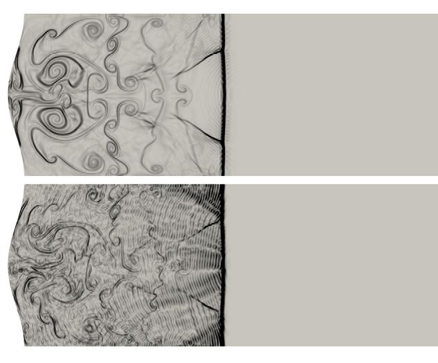
V. C. B. Sousa and C. Scalo                                                                Journal of Computational Physics 459 (2022) 111139

    Concomitantly, a different method called Spectral Vanishing Viscosity (SVV) arose from the question of how to recover
spectral convergence properties when dealing with conservation laws that exhibit spontaneous shock discontinuities. Tad-
mor [48,49] studied the use of Fourier-based discretization methods to solve the inviscid Burgers’ equations and concluded
that, if no regularization term was introduced, the numerical solution would not respect the unique entropy solution and
convergence may not be achieved. He then proposed to introduce a wavenumber-dependent viscosity term that would
prevent oscillations and lead to convergence to the unique entropy solution. The idea was shown to be successful by math-
ematical proofs and numerical experiments. Subsequent work by Karamanos and Karniadakis [19] and Pasquetti [38] applied
it to incompressible turbulent flows, via mere addition of the artificial SVV term to the momentum equation without further
consideration. Additionally, Kirby and Karniadakis [22] applied the same framework to compressible turbulent simulations
and artificial spectral dissipation terms were added to the mass, momentum and energy equations. Although the results
gathered in these previous works show that the simple extension of the SVV, developed to treat shock discontinuities, to
hydrodynamic turbulence works, a clear explanation for the reasons why it worked are lacking. Pasquetti [38] concludes his
work on a similar note stating that, although useful, the SVV-LES approach does not rely on physical arguments and there-
fore it only constitutes an efficient platform with the potential to support an SFS model. The current manuscript addresses
this important conceptual gap in section 2.
    In the current paper, a novel numerical scheme for conducting compressible flow simulations on coarse grids called
Quasi-Spectral Viscosity (QSV) is presented. The scheme is based on solving the filtered Navier-Stokes equations using a
common mathematical approach to model any type of SFS stresses, whether they are due to turbulence or shocks. In
section 2, the connection between previous LES and spectral artificial viscosity methods is highlighted. This is done through
the analysis of the subfilter scale terms present in the filtered Burgers’ equation and their parallel to those present in the
filtered incompressible Navier-Stokes. This establishes the theoretical foundation upon which the Quasi-Spectral Viscosity
(QSV) method is constructed. Following, section 3 discusses the fully detailed implementation of the QSV approach in high-
order finite difference solvers focusing on how to estimate the magnitude of the fluctuations near the grid cutoff and on
how to introduce a wavenumber modulation to the dissipation spectrum by using the residual of spatial filter operators.
Next, in section 4, the compressible filtered Navier-Stokes equations are presented and the QSV-based closure models are
proposed. Subsequently, section 5 focuses on demonstrating QSV’s capability of performing simulations of shock-dominated
flows by studying the Sod shock tube problem, the Shu-Osher shock-entropy wave interaction, a shock/vortex interaction
and shock reflection off a sinusoidal wall. Consecutively, section 6 discusses QSV’s ability of acting as a turbulence model
by analyzing a subsonic Taylor Green Vortex (TGV) test case and compressible turbulent channel flow simulations up to
hypersonic bulk Mach numbers. Ultimately, section 7 assesses the claim of QSV being a unified approach for shock capturing
and turbulence modeling by examining the results obtained from a supersonic TGV test case, exhibiting shock-turbulence
interaction dynamics.

2. Foundations of a united framework for SFS turbulence modeling and spectral shock capturing

   The objective of this section is to highlight overlooked mathematical similarities between previous eddy-viscosity models
and the discontinuity regularization method based on artificial addition of a spectrally vanishing viscosity (SVV) [48,49]. The
new perspective presented hereafter serves as a theoretical justification for the unification of the modeling for hydrodynamic
turbulence and shock discontinuities, as well as a base for building the QSV method, the application of the current idea to
high-order finite difference solvers.

2.1. Similarities between the filtered incompressible Navier-Stokes and the filtered Burgers’ equations

   First, focus is given to hydrodynamic turbulence and its mathematical affinity to wave steepening and discontinuity
formation. The normalized incompressible Navier-Stokes are taken under consideration:

         ∂ ui
              = 0,                                                                                                                       (1)
         ∂ xi
         ∂ ui   ∂ ui u j    ∂P     1 ∂ 2ui
              +          =−      +                ,                                                                                      (2)
          ∂t     ∂xj        ∂ xi   Re ∂ x j ∂ x j

where P = p /ρref U ref
                    2
                        and u i are the velocity components nondimensionalized by U ref . These equations are then filtered by
an operation that commutes with the derivation,

         f (x) =        f (x )G (x, x )dx ,                                                                                           (3)

with an associated filter width () resulting in the filtered incompressible Navier Stokes:

         ∂ ui
              = 0,                                                                                                                       (4)
         ∂ xi
                                                                  3
V. C. B. Sousa and C. Scalo                                                                                Journal of Computational Physics 459 (2022) 111139

         ∂ ui   ∂ ui u j    ∂P     1 ∂ 2ui          ∂ τi j
              +          =−      +                −        ,                                                                                             (5)
          ∂t     ∂xj        ∂ xi   Re ∂ x j ∂ x j   ∂xj
where, τi j = u i u j − u i u j is the subfilter scale (SFS) stress tensor, a remainder of the filtering operation applied to the
nonlinear governing equations. Since the SFS term depends on the unresolved scales in the flow, it must be modeled. The
modeling hypothesis is that the energy flux between the resolved scales and the subfilter scales can be parametrized as
akin to a momentum diffusion process:

             ∂ τidj
                  ∂                        d            1                    1       ∂ ui   ∂u j
         −     =     2νt S i j ,          τ = τi j − τkk δi j ,
                                           ij                        Sij =                +            ,                                                 (6)
           ∂xj   ∂xj                                    3                    2       ∂xj    ∂ xi
where the superscript ‘d’ indicates the deviatoric components and where νt is the eddy viscosity, previously discussed in
section 1. In incompressible LES, the trace of the subfilter stress tensor (τkk ) is absorbed into the pressure term. Now, if one
uses the same framework to derive the filtered version of the inviscid Burgers’ equation, a prototypical representation of
nonlinear scalar conservation laws that develops a discontinuity in a finite time, the result is:

         ∂ u1 1 ∂ u1 u1                    ∂ u1 1 ∂ u1 u1    1 ∂ τ11
             +          = 0,                   +          =−         .                                                                                   (7)
          ∂t   2 ∂ x1                       ∂t   2 ∂ x1      2 ∂ x1
Because of its simplicity, its parallel with the LES framework and its connection to solutions with discontinuities, the Burgers’
equation will be used as a test case for the Dynamic Smagorinsky (DYN), the Spectral Eddy Viscosity (SEV) and the SVV
models. Previously, an overview of these models and their connection is provided.

2.2. Unified mathematical formulation for eddy and spectral artificial viscosity methods

    One starts by introducing the Germano et al.’s [14] dynamic procedure (DYN), a way of instantaneously modulating the
intensity of the SFS terms by comparing the energy content present in fields filtered with different strengths as an strategy
to estimate the energy content of the smallest resolved scales. This extra step leads to the addition of a modulating factor
C , active only when the scales present in the flow surpass the threshold of the stronger (test) filter. This resolves issues
typically associated with the plain Smagorinsky model, which introduces excessive damping during flow transition and does
not vanish at the boundaries in wall-bounded flows. In a simplified equation format it can be written as
                          2
         τidj = −2C  | S i j | S i j .                                                                                                                  (8)

   Another model of interest is the Spectral Eddy Viscosity (SEV) model proposed by Chollet and Lesieur [5]. First, one starts
with the sharp spectral filtered momentum equation in Fourier space,

             ∂
                + (ν + νt (k, kc ))k
                                    2
                                        u (k, t ) = t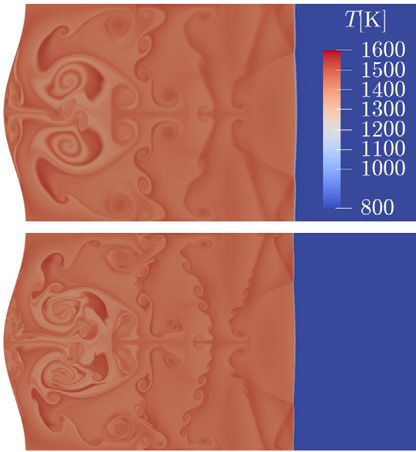
V. C. B. Sousa and C. Scalo                                                           Journal of Computational Physics 459 (2022) 111139

Note that the reformulation of the SEV model in the physical space makes its connection to Germano et al.’s [14] dy-
namic procedure more clear: both models effectively apply test filters on the resolved scales to inform the modeling of the
unclosed terms. The difference being that the SEV model imposes a plateau-cusp shape to the residual of its related test
filter by working in spectral space, whereas test filters are used in the dynamic procedure only to control the dissipation
magnitude.
   Additionally, such a perspective change can elucidate that fact that, if the residual of a filtering operation can be used as
a wavenumber modulation function for the eddy viscosity, one would be able to implement such a model as a function of
physical space operators rendering it possible to be implemented in high-order finite difference frameworks. This is one of
the key elements of the Quasi-Spectral Viscosity’s (QSV) approach, which will be further discussed in section 3.
   Ultimately the Spectral Vanishing Viscosity (SVV) [48,49] method is addressed. It consists of adding an artificial dissipa-
tion term to the Burgers’ equation with the aim to regularize its solutions and enable spectral convergence properties away
from the discontinuity region. The method reads in physical space as,

         ∂ u 1 ∂ uu   ∂                     ∂u
            +       =                 Q ∗        ,                                                                                (13)
         ∂t   2 ∂x    ∂x                    ∂x
where Q is a viscosity kernel. Looking at such a formulation, one notes its similarity with the filtered Burgers’ equation (7),
derived using the LES-based idea of solving only for the large scales and modeling the energy flux to the sub-filter scales
(SFS). In conclusion, although previously unnoticed, the addition of the SVV artificial viscosity component is akin to the
inclusion of an eddy-viscosity term (such as in the previously discussed DYN and SEV models), with the difference being
the specific spectral make-up of the modeled unresolved terms.
   During the development of the SVV model, Tadmor [48,49] applied a Fourier transform to equation (13) and proved that
the dissipation action by Q leads stability and spectral accuracy away from the discontinuity if

                1                                    1
                       and   F[Q ] =
                                      Q  Const −         .                                                                       (14)
               kc                                    k2
From these, he interpreted that the minimum “artificial” dissipation needed to ensure spectral accuracy would need to be
                                                                                                     β
  ≈ k1c and could be made to only act in modes above a certain activation wavenumber m ∼ kc , with β < 12 , rendering
most of the spectrum inviscid, as in equation (15). Here it should be pointed out that a formulation where Q affects all the
scales, i.e. m = 0, is also consistent with the theoretical results, as pointed out by Karamanos and Karniadakis [19] and that
1/kc is effectively an estimate for the length scale at the cutoff, as pointed out in the previous subsection.
   Tadmor’s [48,49] first proposed SVV implementation was

               0, if |k|  m

         Q =                                                                                                                      (15)
               1, otherwise

which we note that, consistently with the spirit of this √
                                                         section, can also be implemented as the residual of a sharp spectral
test filter operation. His results, performed with m = 2 kc , showed that the application of the regularization term made a
previously unstable simulation converge. Moreover, it was noted that C ∞ smoothness of the viscosity’s kernel wavenumber
dependency improved the resolution of the method.
   In a subsequent work, Maday et al. [29] analyzed the Burgers’ equation in the context of a Legendre pseudo-spectral
method and proved that the use of a SVV regularization term lead also to convergence to the exact entropy solution. In
order to improve SVV’s performance, Maday et al. [29] proposed a viscosity kernel of the form

              e −(k−kc ) /(k−m)
                        2       2

                                       if |k| > m
         Q =                                                                                                                      (16)
               0,                       otherwise
                    √
where m = 5 kc and = kc−1 . In this form, a vanishing viscosity magnitude, which decreases continuously as the mode
number decreases, is obtained.
   In summary, all the presented models, after some changes in perspective, fit into a generalized format of subfilter scale
flux modeling consisting of a magnitude pre-factor composed by a length scale () and velocity a velocity scale (υc ) plus a
kernel (K ) which is convolved with the strain rate tensor (S i j ), as in

         τi j = υc K ∗ S i j .                                                                                                   (17)
Table 1 emphasizes the connection between the dynamic procedure (DYN), the SEV and the SVV methods and how they
relate to the generalized form (17). Table 1 also foreshadows the QSV’s closure (explained in section 3), which can be loosely
interpreted as the extension of the SEV methodology to high-order finite difference implementations in physical space.
    Although the current manuscript is focused on applications based on structured finite difference solvers, the contents of
this section may serve as the foundation for the application of an unified approach to shock capturing and SFS turbulence
modeling to different platforms, such as unstructured block-spectral solvers.

                                                              5
V. C. B. Sousa and C. Scalo                                                                               Journal of Computational Physics 459 (2022) 111139

                                        Table 1
                                        Summary of different eddy and artificial viscosity models and their connec-
                                        tion to a generalized formulation.

                                                   Length Scale ()      Velocity Scale (υc )    Kernel (K )
                                         DYN                            2C | S i j |           1

                                         SEV       1/kc                      kc E kc             F −1 [νt+ (k/kc )]
                                         SVV                             1                       Q

                                         QSV                                2E kc /            1 − G qsv

2.3. Analysis of the numerical solution of the filtered Burgers’ equation

    The Burgers’ equation is integrated in the periodic domain x1 ∈ [−1, 1], starting from the initial conditions
                                1
         u 1 (x, t = 0) = 1 +       sin(π x),                                                                                                         (18)
                                2
until t = 1 using a pseudo-spectral Fourier method for the spatial derivatives and a 4th order Runge-Kutta scheme for the
time integration. The results obtained using the different eddy viscosity closures are then compared with the analytical
solution based on the method of characteristics in the physical and spectral domain. In the current work, the procedure
of comparing simulated results to a reference solution will be referred to as a posteriori analysis. In addition, an a priori
analysis is also conducted. It is defined as an operation that filters the exact solution and its nonlinear terms at a certain
time instant by a sharp spectral transfer function down to the same resolution as the numerical simulations performed. This
allows the comparison between the exact SFS stress, u i u j − u i u j , and the output of each different model when the exact
filtered solution u i is used as input. The intent of this operation is to exploit the access to a reference solution to calculate
τi j explicitly, the term that needs to be modeled to sustain a filtered solution of a given equation, and assess each model’s
ability to generate similar effects while only having access to the information present on the large flow scales.
     It can be observed, in 1 b) that the exact energy flux to the sub-filter scales (blue line) spans across all resolved
wavenumbers and it peaks near the cutoff (kc ). This resembles the plateau-cusp behavior of the SEV model for hydrody-
namic turbulent flows [5,23] but observed in the context of a shock-formation phenomena. These results, therefore, can
be regarded as another argument in favor of the unification of shock capturing and (hydrodynamic) turbulence modeling
methods.
     Now focus is given to the performance of the different models. First, it can be noted in Fig. 1 that the localization in
physical space of the dynamic Smagorinsky procedure leads to a flat broadband response in the wavenumber space that
overestimates dissipation at the large scales and underestimates it at scales near the filter’s cutoff when modeling the SFS
stress. The result of this spectral behavior when used to perform filtered simulations of inviscid Burgers’ equation leads
to spurious high-wavenumber build up due to the insufficient damping of the resolved scales near the cutoff. This is an
undesirable behavior since it affects the overall accuracy of the solution in physical space, as observed by the presence of
artificial high frequency oscillations.
     Following, the a priori analysis of the SEV method shows that the growth of the magnitude of the modeled SFS stress
components near the grid cutoff is able to follow more closely what is observed in the exact SFS stress although a certain
degree of overdamping is introduced. In physical space, the dissipation’s cusp behavior near the cutoff leads to τ11 being
slightly non-local, following some of the oscillatory behavior of the analytical result. Moreover, the a posteriori results show
that, in spite of some slight energy build up near the cutoff, the filtered solution follows the energy cascade of the exact
solution closely. In the physical space, a mostly monotonic solution is achieved, with only low amplitude high frequency
oscillations at the cutoff wavelength.                                                                 √
     The SVV method is then analyzed by using both the suggested activation wavenumber m = 5 kc as well as m = 0. By
studying the model in an a priori analysis, one can observe that the tentative of leaving part of the spectrum inviscid always
leads to underdamping in the low wavenumber range. This reflects in the a posteriori solution as different degrees of energy
accumulation near the cutoff in spectral space and oscillations near the discontinuity in the physical space solution. More-
over, when a larger portion of the spectrum is left inviscid, the level of energy accumulation and amplitude of oscillations
are higher. This effect is not limited to the solution of Burgers’ equation, as energy pile-up at high wavenumbers was also
observed by Andreassen et al. [1], while using the SVV method to perform simulations of waves in a stratified atmosphere.
     Despite not being the optimal way of introducing a spectral viscosity term, the SVV method does indeed lead to stable
and accurate solutions as proved by Tadmor [48]. SVV paves a strong numerical theoretical background for the implementa-
tion of a spectral viscosity term in any hierarchical set of basis functions and its direct connection to the LES mathematical
framework clarified in the current manuscript aims to widen its applications and strengthen its technical background when
not applied to the initial setup where it was developed. Some examples of implementations of the standard SVV model
using different methods are the Fourier [48,49], Legendre [29], Chebyshev Andreassen et al. [1] and multi domain spectral
methods, based on the spectral/hp Galerkin approach, by Karamanos and Karniadakis [19]. Similarly, SEV-type models, ini-
tially developed in the Fourier spectral space, can be extended to a different spectral orthogonal basis set. This has not been
addressed in previous literature.

                                                                              6
V. C. B. Sousa and C. Scalo                                                                                   Journal of Computational Physics 459 (2022) 111139

Fig. 1. Results from a priori and a posteriori analysis of the filtered Burgers’ equation at time t = 1 with N = 128 grid points. Exact SFS stress (blue) compared
against SFS stresses predicted by various models (see legend), in the physical (a) and spectral (b) domain. Exact filtered solution (blue) versus a posteriori
solution by various models (see legend) in the physical space (c) and their respective energy spectrum (d). (For interpretation of the colors in the figure(s),
the reader is referred to the web version of this article.)

    One important conclusion that arises from the analysis of Fig. 1 is that, the closer the spectral content of the added
dissipation is to the exact SFS stresses, the better is the performance of the model in solving for the resolved flow scales.
Because of that, while developing the QSV’s method, the transfer function of G qsv (see Table 1) was tailored to be closer
to the exact SFS flux with the added difficulty of only using physical space operators. The mathematical details underlying
QSV’s method are discussed in section 3.
    Before presenting the inner workings of the QSV’s physical space implementation, it is compared against methods for
eddy and artificial viscosity. The analysis of QSV’s results gathered in Fig. 1 shows a slight energy accumulation at the end
of the resolved spectra, near the cutoff wavenumber. Despite the small pile-up, good agreement between the analytical and
simulated results is recovered in both physical domain and in the slope of the energy cascade in the low wavenumber
range. When compared against the previous mentioned methods, it performs equally well or better in terms of the range of
wavenumbers solved accurately. These results serve as a proof of concept that a spectral-like behavior can be introduced by
the use of residuals of filtering operations.

3. Mathematical formulation of the Quasi-Spectral Viscosity (QSV) closure

    The previous section has established how various eddy and artificial viscosity models can be recast under a common
mathematical formulation (17). This demonstrates that the same principles used by large-eddy simulations of hydrodynamic
turbulence, focusing on simulating only the large, resolved or filtered scales, can be used for discontinuity capturing as well.
Fig. 1 from the previous section further establishes this relation and inspires the Quasi-Spectral Viscosity (QSV) closure, de-
signed specifically to unify the LES and shock capturing methodologies in high-order finite difference implementations. The
current section explains the details of its implementation, applied in section 4 to the Favre-filtered Navier-Stokes equations.
The following sections demonstrate the model’s performance in purely shock-dominated flows, purely turbulent flows and,
finally, flows exhibiting shock-turbulence interactions.
    The Quasi-Spectral Viscosity (QSV) closure can be generically written as,

         −τ =        2 E kc (1 − G qsv ) ∗ S .                                                                                                            (19)

                                                                               7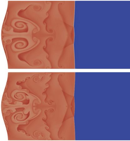
V. C. B. Sousa and C. Scalo                                                                                                   Journal of Computational Physics 459 (2022) 111139

There are two steps for implementing the method: first, estimating the cutoff energy, E kc , and second, introducing a plateau-
cusp behavior as a function of wavenumber, done by the residual filtering operation, 1 − G qsv . For these to be implemented
in a high-order finite difference setting, they need to be performed only using spatial operators, which are discussed in
subsections 3.1 and 3.2.
    Previously, an attempt to extend the SEV model to physical space was also addressed by Metais and Lesieur [31], although
it only focused on the cutoff energy estimation and not on the spectral modulation. Metais and Lesieur [31] used a structure
function to estimate E kc and averaged the viscosity kernel transfer function to be able to apply a constant coefficient in the
wavenumber space. On top of not introducing the plateau-cusp behavior, the relation between E kc and the structure function
is based on turbulence theory, which assumes local isotropy and homogeneity at the small scales. In the current work, a
different approach based on numerical operators, is proposed. Ultimately, the use of numerical theory should relax the
assumptions needed to estimate the cutoff energy and also allow the introduction of a wavenumber modulation.

3.1. Estimation of resolved flow energy at grid cutoff

    The QSV method starts by analyzing the residual field associated with a filter based on Padé operators [24]. A family of
sixth order implicit Padé filters is defined as


                                                            3
                                                              aj
         α f̃ i−1 + f̃ i + α f̃ i+1 = a0 f i +                                ( f i + j + f i − j ),                                                                      (20)
                                                                      2
                                                             j =1

where f is the quantity being filtered, f̃ is the filtered field,                                         α ∈ (0, 0.5) is a parameter which controls the filter’s strength
and its weights defined as a function of α are,
                  11 + 10α                       15 + 34α                             −3 + 6α                 1 − 2α
         a0 =                       , a1 =                      , a2 =                             and a3 =            .                                                  (21)
                       16                             32                                      16               32
From the filter’s definition, one can arrive at its transfer function,


                                                  3
                                      a0 +             a j cos j π kk
                                                                                  c
                          k                      j =1
        G  Pade       α,            =                                                   ,                                                                               (22)
                           kc               1 + 2α cos            π kkc
where kc = π /.
   Fig. 2 shows that the residual of a Padé filter operation can serve as an estimate for the spectral energy content near the
cutoff, i.e.

         E kc ≈ 1 −
                    G Pade ∗ E .                                                                                                                                          (23)

Such residual is a monotonically increasing function of the wavenumber and can be made to concentrate towards the cut-off
kc depending on the value of α . The duality between frequency and physical spaces woven by the Fourier transform, though,
leads to the general principle that a function f (x) and its Fourier transform f̂ (k)) cannot be simultaneously localized in
their own space. This principle is demonstrated in Fig. 2 by showing the physical residual of Padé filters for different
values of α applied to a unitary step function located at x = 0.5. It can be observed that a higher value of α yields a
higher concentration near the cutoff wavenumber in the spectral space, and a corresponding broadening in the physical
space, resulting in a (more) global numerical operation. Ultimately, a trade-off must be found between the accuracy of the
estimation of the spectral energy magnitude near the cutoff and the locality of the resulting operation.
    Initially, only values of α close to 0.5 result in accurate estimation of the energy content near the cutoff but, as discussed,
that leads to highly non-local spatial dissipation. A scaling of the energy at the cutoff is proposed to improve the range of
α that leads to good E kc estimates and, with that, to achieve a higher degree of flexibility in the choice of locality of the
energy estimation operation in the physical space. First, it is noted that the most accurate E kc estimation for a certain grid
discretization using the family of Padé filters is the one for which the inflection point of the transfer function equals to 0.5
at the last resolvable mode prior to the cutoff. This previous statement is equivalent to saying that there exists a maximum
αkc , which satisfies the following relation,

                              kc − 1
        G  Pade       αkc ,                     = 0.5.                                                                                                                    (24)
                                kc
From here, one can solve for the value
                                            αkc using relations (21) and (22). If the residual transfer function achieved by
                                          of
                                          k
using the parameter αkc , 1 − G Pade αkc , k , is integrated, it is possible to define a reference area connected to the best
                                                                          c
estimate for the amplitude of the energy near the cutoff for a certain grid size. In general, this integral is only a function of
α , being

                                                                                                       8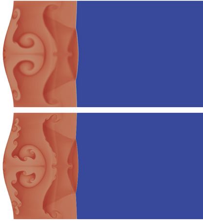
V. C. B. Sousa and C. Scalo                                                                                                                              Journal of Computational Physics 459 (2022) 111139

Fig. 2. Transfer functions obtained for energy at the cutoff operator and the residual of a sixth order Padé filter when kc = 64 (left) are shown together
with the physical space result of a Padé residual operation when applied to a unitary step function located at x = 0.5 (right).

                                                                         ⎧
                         1                                            ⎨ 16
                                                                           5
                                                                              ,                                                                                         if α = 0,
                                 1−

         A (α ) =                  G Pade d(k/kc ) =                             1 −4 α 2 −1 +2 α 2              1−4α 2 −1 +α 14α +2 1−4α 2 −1                                                       (25)
                                                                         ⎩                                                                                            , if 0 < α < 0.5.
                         0                                                                                                 64α 3

   Now, if a more localized scheme for energy estimation is desired, one can scale the resulting residual operation by the
area ratio between the maximum and desired α , reaching the results shown in Fig. 2. Ultimately, in three dimensions, the
residual filtering operation can be applied in the i-th direction to estimate the cutoff energy content of each resolved u j
velocity component,

                                                           (u )2                     A i (α )
                                                               j
         E ki c (u j )   =       1−        Gi     Pade (α ) ∗                                      .                                                                                                 (26)
                                                                        2             A i (αkc )

With this formulation, the information on the magnitude is preserved but the use of lower values of α lead to lower
wavenumbers, or larger scales, being detected by sensor and again a trade-off must be sought. Although an optimal α
might differ for each individual setup, the value of α = 0.45 produces satisfying results for all the problems in the current
manuscript.

3.2. Wavenumber modulation of the added dissipation

   The question of how to estimate the residual energy in physical space was addressed and now the problem of adding
wavenumber dependency on the eddy viscosity term using only spatial operators will be tackled. For this, start by consid-
ering the Vandeven filter of order p = 1 [52],

         σ1 (η) = 1 − η,                                                                                                                                                                             (27)
defined only on the resolved scales, i.e. η ∈ [0, 1]. A filter with such a transfer function was studied by Fejér [12] in the
context of looking for monotonic reconstructions of Fourier series partial sums and will be from now on referred to as Fejér
filter. Such a filter acts by modulating the amplitudes of the various Fourier components as


                         kc
         f σp =                  f̂ k σ p (η) e ikx ,                                                                                                                                                (28)
                    k=−kc

where σ p = 1 results in no filtering. The Fejér filter can be cast as a spatial operator.
   Starting from the spectral filter equation (28) applied to u (x), one substitutes û for the discrete Fourier transform (DFT)
operation,
                                 ⎛                                               ⎞

                     kc
                                                  2k c −1
                                         1                                                        k
         u σ1 =                  ⎝                          u (x j )e   −ikx j ⎠
                                                                                          1−               e ikx ,                                                                                   (29)
                                     2kc ck                                                    kc
                    k=−kc                          j =0

where ck is a term that appears due to aliasing on the last mode, being equal to 1 for |k| < kc , and ck = 2 for k = ±kc [43].
From this one can derive the operator that, when applied to the discrete values of the function, u (x j ), where x j are the
                          2π
colocation points x j = j 2k , 0  j  2kc − 1, return its Fejér filtered value. From equation (29) one has that
                                              c
                                ⎛                                                              ⎞

                    2k c −1                  kc

                                                                                                                         2k c −1
                                     1                            k         1
         u σ1 =                 ⎝                         1−                     e   ik(x−x j ) ⎠
                                                                                                       u (x j ) =                  G Fejer (x − x j )u (x j ).                                       (30)
                                     2kc                         kc         ck
                         j =0                k=−kc                                                                        j =0

                                                                                                                     9
V. C. B. Sousa and C. Scalo                                                                                Journal of Computational Physics 459 (2022) 111139

Fig. 3. The Fejér kernel in space and its self windowed behavior is shown on the left for N = 128. On the right, the related transfer function obtained for
the global (n w = N /2) and for the truncated operators for different window widths n w .

After some algebraic manipulation and using the help from the closed form of the Fejér kernel, the spatial Fejér filter
operator is defined as

                                csc2 θ2
         G Fejer (θ) =                             [1 − cos (kc θ) + sin (kc θ) sin(θ)]                                                                (31)
                           2kc (2kc + 2)
                                                                                    2π
where θ = x − x j . Ultimately, its implementation in a discrete grid where x j = j 2k   , j = 0, 1, ..., 2kc − 1 would be done by
                                                                                       c
solving u = G Fejer,i j u j where
         σ1

                              4+2kc
                                        ,                                                    if i = j
         G Fejer,i j =
                              2(2+2kc )                                                                                                              (32)
                                                           π (i − j )
                                    1
                              2kc (2+2kc )
                                               csc2          2kc
                                                                            (1 − (−1)i − j ), otherwise.
   The thus-obtained closed form is strictly speaking a global periodic operator, i.e. weights should be applied to all points
in one direction periodically to determine the filtered value at one grid location. This is equivalent to performing a filtering
operation in the Fourier spectral space. However, casting it as a spatial operator and truncating its stencil, makes the
operation local in space, allowing its extension to non-periodic boundary conditions.
   To analyze how the truncation operation affects the Fejér filter operator note that, for a centered, explicit and symmetric
scheme, generically represented here as,


                              nw
                                 aj
         G i = a0 G i +                    (G i + j + G i − j ),                                                                                       (33)
                                       2
                               j =1

its transfer function can be represented as

                                  nw
                k                                              k
        G                = a0 +              a j cos       jπ            ,                                                                             (34)
                kc                                              kc
                                      j =1

where kc = π /. Fig. 3 shows that the self windowed nature of the weights of the Fejér filter spatial operator makes its
transfer function converge quickly to the theoretical straight line independently of the number of the total number of modes.
This behavior renders the truncated version of the operator useful. In the current manuscript a stencil size of n w = 8 is used
as the default value, but as the grid points approach a nonperiodic boundary, the window size is decreased accordingly.
   At this point, all the tools necessary to build the effective transfer function used to modulate the magnitude of the
spectral dissipation added to each wavenumber are presented. Recall the results presented in Fig. 1 b): the a priori SFS
dissipation associated with previous models either over or underestimates the exact SFS dissipation at low wavenumbers.
On the other hand, the QSV spectral modulation transfer function is tailored to be close to the plateau-cusp behavior of the
exact SFS energy flux. Such modulation is performed by using only spatial operators through a linear combination of the
residuals of the truncated spatial Fejér filter operator (32) and the previously mentioned Padé filter (22):


        G        = w 1 − β
                          G Pade (α ) + (1 − β)
                                               G Fejer .                                                                                               (35)
           qsv

The values used for the filter strength, α = 0.45, for the weighted average factor, β = 0.8, together with a ‘DC’ offset of
w = 0.85 were used to generate the results gathered in the current manuscript.
    Moreover, it is necessary to note that how these various parameters interact with each other is ultimately described by
the constructed transfer function, shown in Fig. 1 b), and how each component affects such curve can be translated directly
to the model’s behavior. Ultimately, changes in the parameters that lead to small changes in the final modulation curve can
only generate slight differences in the results achieved by the model.
    Although α , β and w seem to be arbitrarily chosen solely based on the Burgers’ test case, their choice has also been
informed by other extracting other exact SFS spectra, such as the ones obtained in the a priori analysis of the Taylor-Green

                                                                                             10
V. C. B. Sousa and C. Scalo Journal of Computational Physics 459 (2022) 111139
Vortex (Fig. 12) and the Riemann shock tube problem (Fig. A.21), leading to good agreement and displaying an expected
universal behavior, being the plateau-cusp shape a theoretical result [5,23]. The suggested values for α , β and w work
well for a wide range of test cases, i.e. shock-dominated (section 5) or turbulence-dominated (section 6) problems, and a
shock-turbulence interaction problem (section 7), however, they might have to be adjusted if different numerical schemes
or filter combinations are adopted. Such values, as well as the choice of spatial filtering operations, may not be optimal, but
they shed light on a novel perspective on how to develop eddy-viscosity models.
Finally, one comment must be made regarding the applicability of the QSV closure here derived. Since the spectral modu-
lation is inspired by an a priori analysis carried out with sharp spectral filters, the model, as constructed, is only suitable for
spectral or quasi-spectral high-order discretizations. A different primary filter, for example the transfer function of a second
order interpolation operator, could be used in a separate a priori analysis to look for an alternative QSV implementation in
low-order codes.
4. Application of the Quasi-Spectral Viscosity closure in the filtered compressible Navier-Stokes equations
In this section, the compressible implementation of large scale simulations focusing on the unification of the treatment
between shocks and turbulent eddies will be discussed. First the governing equations will be derived from the compressible
Navier-Stokes relations using filtering operations and the unclosed terms as well as their closure will be presented.
4.1. Governing equations
The compressible Navier-Stokes system of equations can also be filtered by an operation that commutes with the deriva-
tion, as described by (3), similarly to its incompressible counterpart (5). After the initial filtering, two routes could be
chosen, the Reynolds-based or the Favre-based filtered equations. By using the Reynolds method, all equations in the sys-
tem would require closure models and the role of small-scale density variations would have to be modeled specifically.
Sidharth and Candler [45] argued that modeling the SFS flux in the density field separately could lead to an improvement
in LES of variable-density turbulence. On the other hand, the use of the Favre-based method leads to implicitly solving
density related nonlinear terms by defining the Favre filter operation as,
ρf
f̌ = . (36)
ρ
In the end, solving for the Favre filtered quantities ( f̌ ) simplifies the LES equations for compressible flows. Moreover,
compressible LES implementations based on the Favre-filtered equations were already successfully performed with different
closure models by, for example, Moin et al. [32], Normand and Lesieur [37], Vreman et al. [54] and Nagarajan et al. [36].
In this work, we follow the path of the latter, and derive the Favre-filtered Navier-Stokes relations introducing a pressure
correction based on the subfilter contribution to the velocity advection,
∂ ρ ∂ ρ ǔ j
+ = 0, (37)
∂t ∂xj
∂ ρ ǔ i ∂ ρ ǔ i ǔ j ∂p ∂ μσ̌i j ∂ ρτi j
+ =− + − , (38)
∂t ∂xj ∂ xi ∂xj ∂xj
∂ E ∂( E + p )ǔ j ∂ ∂ Ť ∂ μσ̌i j ǔ i ∂ρC pq j ∂ 1
+ = k + − − ρϑ j + μ , (39)
∂t ∂xj ∂xj ∂xj ∂xj ∂xj ∂xj 2
p 1 1
= E − ρ ǔ i ǔ i − ρτii . (40)
γ −1 2 2
The nonlinear terms that contribute to the energy flux from large to small scales are, the SFS stress tensor,
τi j = u i u j − ǔ i ǔ j , (41)
the SFS temperature flux,
q j = T u j − Ť ǔ j , (42)
the SFS kinetic energy advection,
ϑ j = uk uk u j − ǔk ǔk ǔ j (43)
and the SFS turbulent heat dissipation
11V. C. B. Sousa and C. Scalo Journal of Computational Physics 459 (2022) 111139
∂ σi j u i ∂ σ̌i j ǔ i
= − . (44)
∂xj ∂xj
Subfilter contributions resulting from the nonlinearities involving either the molecular viscosity or conductivity’s depen-
dency on temperature have been neglected following Vreman et al. [54], who showed those are negligible in comparison
against the other terms’ magnitudes. Following Nagarajan et al. [36], ϑ j and are neglected.
4.2. QSV’s methodology applied to SFS modeling of the compressible Navier-Stokes equations
First, the dissipation magnitude tensor is introduced as
Di j = υi (ǔ j ) j , (45)
where j = j is the sub-filter length scale and
2E ki ǔ j
υi (ǔ j ) = c
(46)
i
is the sub-filter velocity scale. Note that the cutoff energy estimation operation is carried out in the i-th spatial direction
(equation (26)) but on the j-th filtered velocity component. A complete model for performing compressible large scale
simulations that could include both shocks and turbulent events is then proposed as,
1 ∂ ü i ∂ ü j
τi j = − C τi j Di j + D ji , (47)
2 ∂xj ∂ xi
∂ T̈
q j = −C q D j j , (48)
∂xj
where the double dot superscript indicates the filter modulated quantities, defined as
∂ ü i ∂ ǔ i
= ∗ 1 − G qsv , (49)
∂xj ∂xj
∂ T̈ ∂ Ť
= ∗ 1 − G qsv , (50)
∂xj ∂xj
where the modulation step is performed in the three directions and G qsv is described in equation (35). It is possible that
the cutoff energy estimation procedure will lead to large variations in space when highly localized flow features, such as
shocks, do not align with the grid or the grid itself is deformed. In those cases, a smoothing procedure, i.e. a gaussian filter
[7], can be performed on the υi (ǔ j ) term.
The values of the pre-factors, C q and C τi j are given by:
1.0, if i = j ,
C τi j = and C q = 0.8. (51)
0.6, if i = j ,
These values are obtained by carrying out a similar a priori analyses as the one performed to inform the coefficients α , β and
w (see subsection 2.3). The magnitude of these constants is informed, though, through the application of such procedure to
test cases such as the 1D Riemann shock tube problem [47] (Appendix A) and the Taylor Green Vortex (TGV) (section 6.1).
The suggested constants (all of unitary value) work well for a broad set of test cases as shown below. However, if different
numerical schemes or filters are used, adjustments might be necessary. In the following, the proposed QSV’s closure will be
compared against existing LES and shock capturing strategies in various flow setups ranging from incompressible turbulence
to shock-dominated flows, including shock-turbulence interaction test cases.
5. Demonstrating QSV’s shock capturing capability
Hereafter, QSV’s ability to simulate flows with discontinuities is demonstrated in canonical test cases such as the Riemann
shock tube [47], the Shu-Osher shock-entropy wave [44], the shock/vortex and shock/sinusoidal-wall interaction problems.
The aforementioned test cases are solved using a 6th-order Padé compact finite difference scheme [24] coupled with a
3rd-order Runge-Kutta time integration method.
12V. C. B. Sousa and C. Scalo Journal of Computational Physics 459 (2022) 111139
5.1. One-dimensional shock dominated flows
The Favre-filtered one-dimensional compressible Euler equations read,
∂ ρ ∂ ρ ǔ 1
+ = 0, (52)
∂t ∂ x1
∂ ρ ǔ 1 ∂ ρ ǔ 1 ǔ 1 ∂p ∂ ρτ11
+ =− − , (53)
∂t ∂ x1 ∂ x1 ∂ x1
∂ E ∂( E + p )ǔ 1 ∂
+ =− ρ C p q1 , (54)
∂t ∂ x1 ∂ x1
p 1 1
= E − ρ ǔ 1 ǔ 1 − ρτ11 , (55)
γ −1 2 2
where the viscous and conductive effects are neglected and where τ11 and q1 are the sub-filter flux terms. If this system of
equations is initialized the following initial conditions in density, velocity and pressure,
[1, 0, 1], if x < 0.0
[ρ , u , p ](x, 0) = (56)
[0.125, 0, 0.1], otherwise,
then, a single shockwave propagating to the right develops and can be sustained by a Dirichlet supersonic inflow boundary
condition on the left and an Neumann outflow boundary condition on the right. As the flow evolves, its exact solution leads
to 4 constant density states separated by a shock, a contact discontinuity and a rarefaction wave, as shown in Fig. 4 at time
t = 0.2. Shocks and rarefaction regions are also seen in the pressure and velocity fields.
The results for this test case, known as the Sod shock tube problem [47], obtained via the QSV model are then compared
against the Local Artificial Diffusivity (LAD) model [7,20,21]. Fig. 4 gathers a grid sensitivity study of the models considered.
Both models appropriately capture the shock and converge to the exact solution as the grid is refined. Nonetheless, the use
of the QSV model leads to slightly sharper discontinuities for a similar grid refinement level.
The LAD implementation requires an explicit Padé filtering step [21] with α = 0.495, probably due to difficulties with
high-wavenumber energy build-up. This step is not required in the QSV method, although, if used, a lower degree of filtering
(i.e. α > 0.495), is already sufficient to control high wavenumber oscillations. The QSV model is shown both with and
without the application of an explicit filter with α = 0.499, in dashed black and solid red, respectively. The explicit filtering
step is able to attenuate spurious high wavenumber oscillations that are present in the results.
Moving forward, another one dimensional canonical problem, the shock-entropy wave interaction [44], is tackled. The
setup comprises a shock wave propagating into a sinusoidally perturbed resting fluid which, upon interaction, are com-
pressed and acoustic waves are generated. The generated waves have sufficient magnitude to induce wave steepening by
themselves and ultimately generate a train of weak shocks downstream of the primary shock. This problem is defined by
the following initial conditions in the domain x ∈ [−1, 1],
[3.857143, 2.629369, 10.333333], if x < −0.8
[ρ , u , p ](x, 0) = (57)
[1.0 + 0.2 sin(5π x), 0.0, 1.0], otherwise.
The initial conditions are advanced up until t = 0.36 using a timestep of δt = 1 × 10⁻⁵ and results are gathered in Fig. 5.
Once more, results are shown for the QSV model with and without the explicit filtering step and for the LAD model
using the same color scheme as in Fig. 4. Additionally, a QSV-based simulation using 4096 points is used as a reference
solution for the problem. Despite starting from a very coarse grid, a monotonic convergence behavior is observed and the
three approaches converge to the reference solution as the grid is refined. One key aspect to be observed in the simulation
of the Shu-Osher problem [44] is how well the trailing-shock density oscillations can be recovered. Both methods display
similar performance in that regard. However, use of the QSV method leads to a sharper shock discontinuity in comparison
with the LAD approach, specially observed in the u profile.
5.2. Two dimensional inviscid strong vortex/strong shock interaction
√
A stationary shock sustained by an inflow velocity of V 0 = 1.5 γ p 0 /ρ0 is initialized at xs = L /2 inside a computational
domain = [0, 2L ] × [0, L ]. Superposed to this base state, a compressible zero-circulation vortex is initialized upstream of
the shock at (x v , y v ) = ( L /4, L /2) with an inner core radius equal to a = 0.075L and an external radius b = 0.175L. This can
be translated as u = u θ (r )êθ + V 0 êx , where r is the radial distance from the center of the vortex and
⎧r
⎪
⎨ a , if r a
u θ (r )
η r b
= − , if a < r b (58)
u θ (a) ⎪
⎩
2 b r
0, otherwise,
13V. C. B. Sousa and C. Scalo Journal of Computational Physics 459 (2022) 111139
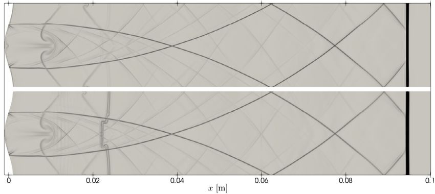
Fig. 4. Sod shock tube results at t = 0.2 computed using the Local Artificial Diffusivity (LAD) method, which requires explicit filtering, and the Quasi-Spectral
Viscosity (QSV) method with and without the explicit filtering operation, are compared against the exact solution.
Fig. 5. Shu-Osher shock entropy wave interaction results at t = 0.36 computed using the Local Artificial Diffusivity (LAD) method, which requires explicit fil-
tering, and the Quasi-Spectral Viscosity (QSV) method with and without the explicit filtering operation, are compared against a reference solution computed
with 4096 points.
14V. C. B. Sousa and C. Scalo Journal of Computational Physics 459 (2022) 111139
Fig. 6. Density isocontours of an inviscid shock/vortex interaction for different grid resolutions for both the Local Artificial Diffusivity (LAD) and the Quasi-
Spectral Viscosity (QSV) methodology.
Fig. 7. Density isocontours of an inviscid shock/vortex interaction using a distorted wavy grid with N x = 384 and N y = 192 points using the Quasi-Spectral
Viscosity (QSV) method.
where η = 2(b/a)/[1 − (b/a)2 ] and the maximum tangential velocity is set to u θ (a) = 0.9V 0 . Following the pressure field is
initialized so that its gradient balances the centripetal force and the following system of equations is solved based on the
ideal gas relation and isentropic compression,
γ
∂P u 2 (r ) P ρ
=ρ θ , P = ρRT , = . (59)
∂r r P0 ρ0
Such a setup was previously introduced by Ellzey et al. [11] to study the structure of the acoustic field generated by
the shock-vortex interaction, by Rault et al. [42] to analyze the driving mechanisms for the production of vorticity in the
interaction at high Mach Numbers and by Tonicello et al. [50] to investigate shock capturing techniques in high-order
methods focused on their influence on the entropy field and its non monotonic profile across a shock.
In the current work, this setup is used to assess the accuracy of the proposed Quasi-Spectral Viscosity (QSV) method.
With that objective, the inviscid shock/vortex interaction was solved at 3 different grid resolution levels, N x = 192; N y = 96,
N x = 384; N y = 192 and N x = 768; N y = 384, using both QSV and the LAD shock capturing scheme [21], being the results
gathered in Fig. 6. Consistently with Rault et al. [42] and Tonicello et al. [50], a highly resolved simulation of such flow
reveals that such a strong shock/strong vortex interaction is a symmetry breaking event resulting in the formation of two
separate counter-clockwise rotating vortices where the bottom one trails behind the top vortex.
The QSV and the LAD models display a similar performance, not being able to capture the asymmetric vortex splitting
event on the coarsest grid but yielding a qualitatively correct solution at the intermediate resolutions. Ultimately, both
methods converge to the same result, as shown in the bottom row of Fig. 6. Despite the similarities, some differences can
be spotted. The QSV-based results display a sharper shock front and lower noise than the ones performed with LAD for grid
sizes N x = 384; N y = 192 and N x = 768; N y = 384. However, the QSV model underestimates the post-shock top vortex core
size on the intermediate grid with respect to LAD.
Following, the original computational domain for the shock-wave/vortex interaction test case, = [0, 2L ] × [0, L ], was
distorted by adding a sinusoidal component in both directions where the following linear mapping,
2π 2π
(xd , yd ) = x + 0.05L sin y , y + 0.05L sin x (60)
L L
relates the original (x, y ) to the distorted grid (xd , yd ). To solve the compressible Navier-Stokes system of equations with
the added closure terms from the QSV model in such a nonorthogonal grid, a curvilinear grid transformation such as in
15You can also read