S-velocity model and inferred Moho topography beneath the Antarctic Plate from Rayleigh waves
←
→
Page content transcription
If your browser does not render page correctly, please read the page content below
S-velocity model and inferred Moho topography beneath
           the Antarctic Plate from Rayleigh waves
     Meijan An, Douglas Wiens, Yue Zhao, Mei Feng, Andrew Nyblade, Masaki
              Kanao, Yuansheng Li, Alessia Maggi, Jean-Jacques Lévêque

     To cite this version:
    Meijan An, Douglas Wiens, Yue Zhao, Mei Feng, Andrew Nyblade, et al.. S-velocity model and
    inferred Moho topography beneath the Antarctic Plate from Rayleigh waves. Journal of Geophysical
    Research, American Geophysical Union, 2015, �10.1002/2014JB011332�. �hal-01239998�

                                 HAL Id: hal-01239998
                https://hal.archives-ouvertes.fr/hal-01239998
                                    Submitted on 21 Oct 2021

    HAL is a multi-disciplinary open access            L’archive ouverte pluridisciplinaire HAL, est
archive for the deposit and dissemination of sci- destinée au dépôt et à la diffusion de documents
entific research documents, whether they are pub- scientifiques de niveau recherche, publiés ou non,
lished or not. The documents may come from émanant des établissements d’enseignement et de
teaching and research institutions in France or recherche français ou étrangers, des laboratoires
abroad, or from public or private research centers. publics ou privés.
                                              Copyright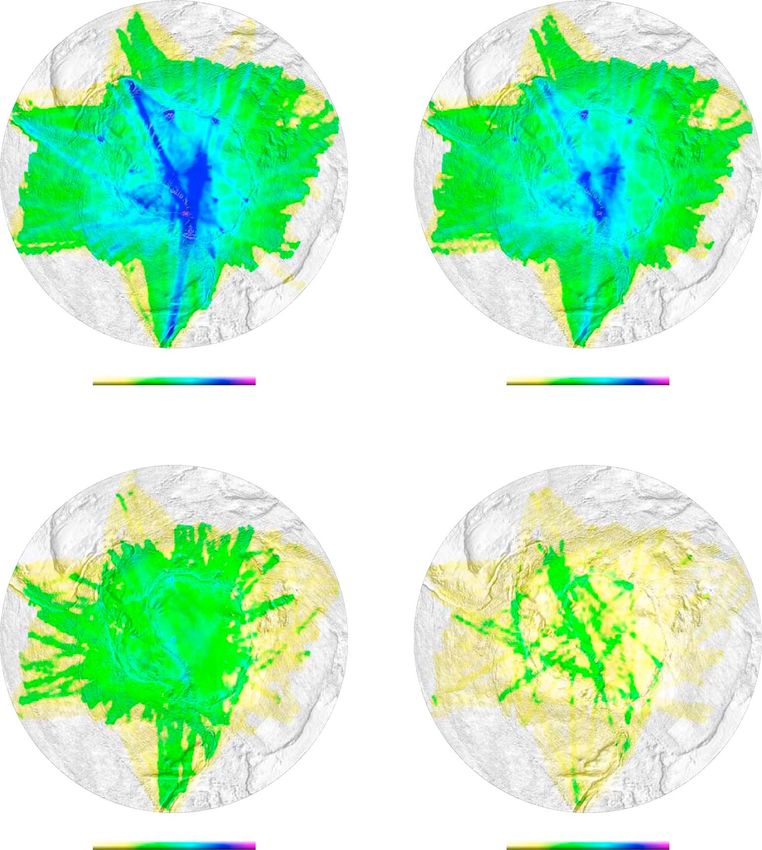
PUBLICATIONS
Journal of Geophysical Research: Solid Earth
RESEARCH ARTICLE                            S-velocity model and inferred Moho topography
10.1002/2014JB011332
                                            beneath the Antarctic Plate from Rayleigh waves
Key Points:                                 Meijian An1, Douglas A. Wiens2, Yue Zhao1, Mei Feng1, Andrew A. Nyblade3, Masaki Kanao4,
• High-resolution crust/lithosphere
  Vs model covering the whole               Yuansheng Li5, Alessia Maggi6, and Jean-Jacques Lévêque6
  Antarctic Plate                           1
• Lithospheric mantle in most of             Institute of Geomechanics, Chinese Academy of Geological Sciences, Beijing, China, 2Department of Earth and Planetary
  the Antarctica is significantly old        Science, Washington University, St. Louis, Missouri, USA, 3Department of Geosciences, Pennsylvania State University,
  and buoyant                               University Park, Pennsylvania, USA, 4National Institute of Polar Research, Tokyo, Japan, 5Polar Research Institute in China,
• East Antarctic Mountain Ranges are
                                            Shanghai, China, 6Institut de Physique du Globe de Strasbourg, Université de Strasbourg/EOST, CNRS, Strasbourg, France
  a thick-crust belt

Supporting Information:                     Abstract Since 2007/2008, seismographs were deployed in many new locations across much of Antarctica.
• Figure S1                                 Using the records from 122 broadband seismic stations, over 10,000 Rayleigh wave fundamental-mode
• Figure S2
                                            dispersion curves have been retrieved from earthquake waveforms and from ambient noise. Using the
• Figure S3
• Figure S4                                 processed data set, a 3-D S-velocity model for the Antarctic lithosphere was constructed using a single-step
• Figure S5                                 surface wave tomographic method, and a Moho depth map was estimated from the model. Using the derived
• Figure S6
                                            crustal thicknesses, the average ratio of lithospheric mantle and crustal densities of Antarctica was calculated.
• Figure S7
• Table S1                                  The calculated density ratio indicates that the average crustal density for Antarctica is much higher than the
• Text S1                                   average values for continental crust or the average density of lithospheric mantle is so low as to be equal to
                                            low-density bound of Archean lithosphere. The latter implies that the lithospheric mantle in much of Antarctica
Correspondence to:
                                            should be old and of Archean age. The East Antarctic Mountain Ranges (EAMOR) represent a thick crustal
M. An and D. A. Wiens,
meijianan@live.com;                         belt, with the thickest crust (~60 km) located close to Dome A. Very high velocities can be found at depths
doug@seismo.wustl.edu                       greater than 200 km beneath parts of East Antarctica, demonstrating that the continental lithosphere extends
                                            deeper than 200 km. The very thick crust beneath the EAMOR may represent the collision suture of East
Citation:                                   Gondwana with Indo-Antarctica and West Gondwana during the Pan-African orogeny.
An, M., D. A. Wiens, Y. Zhao, M. Feng,
A. A. Nyblade, M. Kanao, Y. Li, A. Maggi,
and J.-J. Lévêque (2015), S-velocity
model and inferred Moho topography          1. Introduction
beneath the Antarctic Plate from
Rayleigh waves, J. Geophys. Res. Solid      Antarctica (Figure 1) was part of the Gondwana supercontinent and was contiguous with other present-day
Earth, 120, 359–383, doi:10.1002/           continents (e.g., Africa, India, and Australia) prior to the breakup of Gondwana in the Late Mesozoic [Torsvik
2014JB011332.
                                            et al., 2010], see short overview on the evolution of the continent in the supporting information of this paper.
                                            The continent is mostly covered by ice sheets at present and is moving with only a slight rotational component
Received 28 MAY 2014
Accepted 12 DEC 2014                        in an absolute velocity reference frame [Bouin and Vigny, 2000; Torsvik et al., 2008]. Intracontinental seismicity is
Accepted article online 18 DEC 2014         in a low level [Reading, 2007], even in the West Antarctic rift system (WARS) [Winberry and Anandakrishnan,
Published online 27 JAN 2015
                                            2003; LeMasurier, 2008]. The above conditions imply that no significant tectonic deformation of crust or
                                            lithosphere is presently occurring beneath the ice-covered continent: this is particularly true beneath East
                                            Antarctica (EANT). As such, information regarding its evolution, e.g., the amalgamation and evolution of the
                                            Gondwanaland (~550–200 Ma) and even of the prior Rodinian (~1100–750 Ma), may be still preserved in the
                                            crust and lithospheric mantle of Antarctica.
                                            An understanding of the crustal and upper mantle structure of the Antarctic Plate is essential for understanding
                                            the mechanisms responsible for the assembly and breakup of Gondwana and the dynamics of plate motions
                                            since the Late Mesozoic [Sutherland, 2008; Torsvik et al., 2008]. However, geophysical data collection in the
                                            continent has been hindered by a combination of ice cover and logistical constraints [Bell, 2008; Block et al.,
                                            2009]; e.g., no broadband seismic stations were present on the broad interior area of EANT prior to 2007. The
                                            limited amount of intraplate seismicity has hindered passive-source seismological studies of the
                                            Antarctic lithosphere.
                                            Since the Fourth International Polar Year (IPY) (2007–2008), intensive surveys have been conducted in
                                            Antarctica. In seismology, the Antarctic Network (ANET)–Polar Earth Observing Network (POLENET) project
                                            (2007 to present) significantly improved the coverage of seismic observations in West Antarctica (WANT). The
                                            Gamburtsev Antarctic Mountains Seismic Experiment (GAMSEIS, 2007–2010), part of Antarctica’s Gamburtsev
                                            Province (AGAP) IPY project, involved deployment of broadband seismic stations (Figure 1) in EANT,

AN ET AL.                                                 ©2014. American Geophysical Union. All Rights Reserved.                                                  359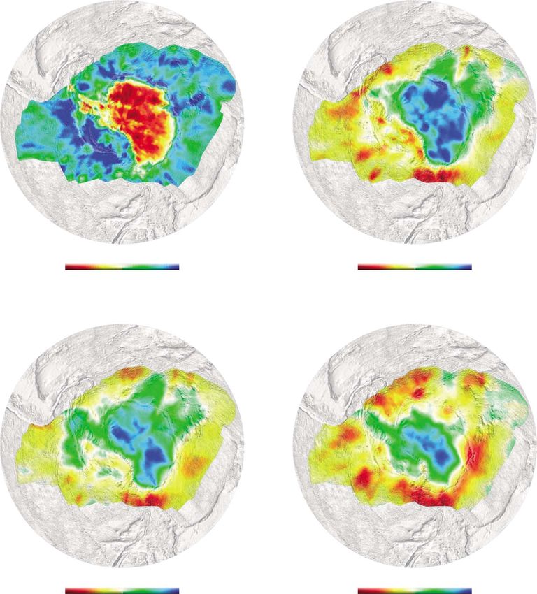
Journal of Geophysical Research: Solid Earth 10.1002/2014JB011332
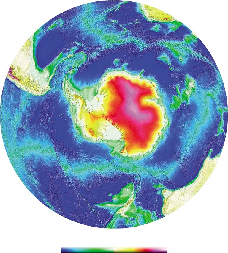
Figure 1. Topography of the Antarctic Plate. The shading is the surface topography from ETOPO2. All broadband seismic
stations (triangles) and earthquakes shown are used in this study. A = Dome A (Argus), AFR = African Plate, AIS = Amery ice
shelf, AmH = American Highland, AUS = Australian Plate, C = Dome C (Circe, Charlie), EANT = East Antarctica, ElL = Ellsworth
Land, EnL = Enderby Land, F = Dome F (Fuji), GSM = Gamburtsev Subglacial Mountains, MBL = Marie Byrd Land,
NAZ = Nazca Plate, NeS = New Schwabenland, PAC = Pacific Plate, QML = Queen Maud Land, rIS = Ronne ice shelf,
RIS = Ross ice shelf, SAM = South American Plate, TAM = Transantarctic Mountains, and WANT = West Antarctica. The
red circles are proposed hot spots at Foundation [Ito and van Keken, 2007], St. Paul Island [Müller et al., 1993], and elsewhere
[Courtillot et al., 2003]. Hot spot abbreviations: Bal = Balleny, Bou = Bouvet, Mar = Marion, and STP = St. Paul-Amsterdam.
Volcanoes were identified by the Global Volcanism Program of the Smithsonian Institution [Siebert and Simkin, 2002].
particularly in the Gamburtsev Subglacial Mountains (GSM) around Dome A (Dome Argus or Kunlun station),
by the United States, China, and Japan. The Chinese stations are under the management of the Chinese
Program of Antarctic Nova Disciplines Aspects. The GAMSEIS stations were located across previously
unexplored areas of the interior of EANT. Data from all GAMSEIS stations in EANT and backbone ANET stations
in WANT used here (Figure 1) are providing important information on the Antarctic Plate.
Surface waves propagating along the Earth’s surface from source to receiver can be used to infer crustal and
lithospheric structure beneath the propagation path, particularly in regions with a paucity of receiving
stations and low seismicity, such as in Antarctica. Therefore, surface wave observations have been widely
applied to the study of crustal and lithospheric structure [e.g., Evison et al., 1960; Dewart and Toksöz, 1965;
Knopoff and Vane, 1978; Roult et al., 1994; Danesi and Morelli, 2001; Ritzwoller et al., 2001; Lawrence et al., 2006]
and crustal thicknesses [e.g., Evison et al., 1960; Ritzwoller et al., 2001; Lawrence et al., 2006] beneath
Antarctica. Surface wave studies of the Antarctic Plate prior to the Fourth IPY [e.g., Danesi and Morelli, 2001;
Ritzwoller et al., 2001] have been severely restricted by the sparse seismic station distribution; thus, to more
robust data requires a denser distribution of seismographs, particularly in the continental interior [Morelli and
Danesi, 2004]. New observations obtained since the Fourth IPY not only permit investigation of regional
AN ET AL. ©2014. American Geophysical Union. All Rights Reserved. 360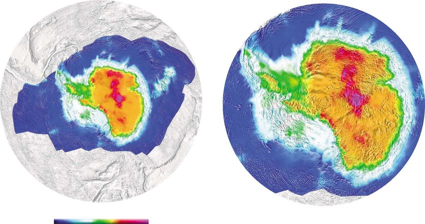
Journal of Geophysical Research: Solid Earth                                             10.1002/2014JB011332

                 crustal structures beneath the stations by receiver function analysis [e.g., Winberry and Anandakrishnan,
                 2004; Bayer et al., 2009; Hansen et al., 2009, 2010; Finotello et al., 2011; Chaput et al., 2014; Feng et al., 2014]
                 but also provide better lateral resolution of surface waves at regional scale study around the GSM [Heeszel
                 et al., 2013] and throughout the entire Antarctic Plate (this study), especially covering the regions, e.g.,
                 from Queen Maud Land (QML) to Ellsworth Land (EL), where the underlying crust and lithosphere have
                 never been well studied by robust seismic exploration.
                 The main objective of this study is to construct a 3-D crustal and lithospheric seismic model for the entire
                 Antarctic Plate using Rayleigh wave group velocities from the seismic waveforms (from earthquake and
                 ambient noise) recorded by Antarctic seismic stations. Upper mantle S-velocity can be converted into
                 temperature that more directly provides tectonic and geodynamic information than seismic velocity [Goes
                 et al., 2000; McKenzie et al., 2005; An and Shi, 2006, 2007]. The mantle temperatures inferred from the
                 S-velocity model of this study are introduced in a later paper of M. An et al. (manuscript in preparation, 2014).
                 The topography and character of seismic discontinuities provide important insights into crustal evolution. The
                 Moho discontinuity at the base of the crust, first identified by Mohorovičić [1910], separates lighter granitic
                 continental crust or basaltic oceanic crust from denser peridotitic upper mantle. Crustal thickness variations of
                 Antarctica have been explored for decades [e.g., Evison et al., 1960; Lawrence et al., 2006; Baranov and Morelli,
                 2013], but until the Fourth IPY, the data were not sufficient to provide a crustal thickness map at reasonable
                 resolutions covering all of Antarctica because most of broad EANT has never been measured. Even after the IPY,
                 the Moho at some of the EANT has not been directly measured yet. Gravity observations are often used to
                 define the relative topography of the Moho [Block et al., 2009; O’Donnell and Nyblade, 2014] using constraints
                 provided where available from high-resolution Moho determinations. Active seismic and receiver function
                 studies provided constraints on crustal thickness in Antarctica below seismic lines or recording stations
                 [Baranov and Morelli, 2013, and references therein]. However, there is also merit in employing techniques, such
                 as analyses of surface waves, that infer crustal thickness along wave propagation path which enable a broader
                 coverage to be obtained. This is important in the case of the Antarctic continent where station coverage is
                 sparse and no robust seismic exploration has yet been conducted in some regions. Here we construct a crustal
                 thickness map for all of Antarctica (including unexplored areas) from the 3-D S-velocity model for the Antarctic
                 Plate. This Moho map greatly improves the resolution of crustal thickness variations across Antarctica compared
                 to previous crustal thickness models of the entire Antarctic continent.

                 2. Data
                 The seismic data used in this study are fundamental-mode Rayleigh wave group velocity measurements from
                 earthquake waveforms and from interstation Green’s functions derived using ambient noise cross correlation.
                 To decrease the position error caused by station movement with underlying ice (e.g., with a rate of up to
                 hundreds of meters per year) or reinstallation [An et al., 2014], we estimated the positions of GAMSEIS stations
                 using year-round GPS records of the stations separated by field service time.
                 Vertical-component seismograms from events with a range of magnitudes and depths were selected for
                 processing based on large theoretical amplitudes calculated from magnitude and event-station distance.
                 Interstation Green’s functions are obtained by cross correlation from vertical-component ambient noise.
                 Rayleigh wave group velocities were measured from the seismograms and Green’s functions using a multiple
                 filtering technique [Dziewonski et al., 1969] with phase-matched processing [Herrin and Goforth, 1977] to
                 isolate the fundamental-mode surface waves. We used a modified program of do_mft from Herrmann and
                 Ammon [2002], in which instantaneous frequency is preferred, in order to take into account the spectral
                 amplitude variation [Nyman and Landisman, 1977] for each nominal frequency of analysis. The primary
                 modification was the use of a filter whose width varies with the filtered period [Feng et al., 2004].
                 The number and distribution of dispersion measurements can directly influence the reliability of the final
                 inverted S-velocity model. Here we provide a brief description of our retrieved data set. We only used the
                 dispersion measurement when the entire propagation path is south of latitude 24°. We retrieved 10,160
                 valid dispersion curves, which are from 122 broadband seismic stations and from 1917 earthquakes
                 (Figure 1) prior to March 2013. Figure 2a shows the number of Rayleigh wave group velocities used for each
                 period. The measurements from ambient noise (Figure 2a) are a small part of all measurements used here.

AN ET AL.                     ©2014. American Geophysical Union. All Rights Reserved.                                            361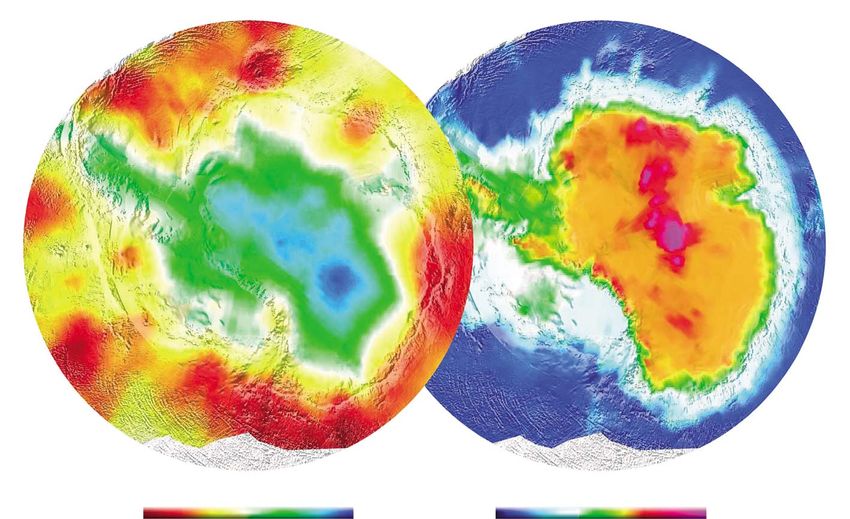
Journal of Geophysical Research: Solid Earth                                                                               10.1002/2014JB011332

                 (a)                            104                                                                  The number of all measurements was 9187
                                                                                                                     for a period of 28 s, and the number of
                                                                                                                     measurements for short (60 s) was much smaller than those
                                                                                                                     for intermediate periods (20–60 s). Figure 2b
                                                103                                                                  shows the maximum period of the dispersion
                                                                                                                     measurements at each position. Figure 3
                                                                                                                     presents a lateral discretization of the study
                                                                                                                     region in the form of equal-area pentagonal
                                                                                                                     and hexagonal cells along with the path-density
                                                                                                                     distribution for periods of 30, 50, 100, and
                                                102
                                                                                                                     150 s. Most continental regions have a density
                                                                                                                     of >50 rays per ~120 km cell at intermediate
                                                      10                                          100
                                                                            Period (s)                               periods (20–60 s) and >10 rays at long periods
                                                                                                                     of 100 s (Figure 3). The dense path coverage at
                 (b)                                                                                                 periods of 20–60 s ensures a good resolution
                                                                                                                     in the resultant model at depths around the
                                                                                                                     continental Moho discontinuity, given that
                                                                                                                     the continental crust is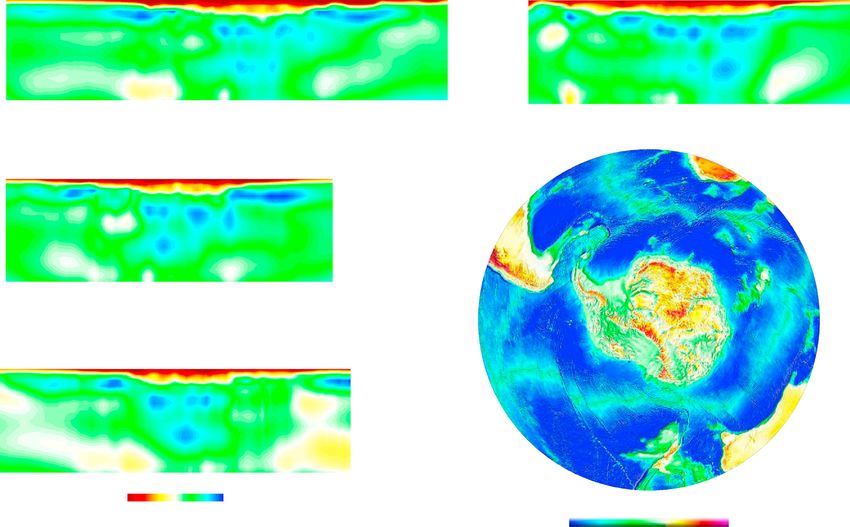
Journal of Geophysical Research: Solid Earth                                                    10.1002/2014JB011332

                 Figure 3. Propagating path density of group velocity measurements at periods of (a) 30 s, (b) 50 s, (c) 100 s, and (d) 150 s.
                 The study region was laterally discretized as equal-area cells, which are bordered by red lines in Figure 3a and which have a
                 great circle extent of ~1° (1° = 111 km). The path density is defined as the number of propagation paths that intersect each
                 cell. Other features in the figure are the same as in Figure 1.

                 The primary improvement of the method used here over Feng and An [2010] is to use equal-area pentagonal
                 and hexagonal cells [Sahr et al., 2003] in horizontal (Figure 3a) rather than traditional quadrangular cells,
                 because equal-area cells are better than quadrangular cells for tomographic studies in polar regions. To
                 adopt a cell with a complex form such as a pentagon or hexagon, most of the basic tomographic procedures
                 for ray tracing through to model appraisal have to be redesigned. For example, new methods need to be
                 developed to estimate model spatial resolution [An, 2012], because simple checkerboard synthetic tests
                 cannot be used for pentagonal and hexagon cells. A secondary improvement is to use Moho discontinuity
                 data as constraints, which is introduced below.

                 3.1. Spatial Resolution
                 We retrieved resolution dimensions for the seismic model by simple methods proposed specifically for this
                 study by An [2012]. The detailed spatial resolution analysis and resolution information can be found in the

AN ET AL.                      ©2014. American Geophysical Union. All Rights Reserved.                                                   363
Journal of Geophysical Research: Solid Earth                                          10.1002/2014JB011332

                 supporting information of this paper. Here we give a short summary of the models’ spatial resolution lengths
                 which are defined as half of the recovered dimension.
                 We first retrieve quantitative resolution lengths for the 2-D surface wave dispersion measurements, which are
                 useful in evaluating the lateral resolution of a surface wave study, by using the statistical resolution length
                 calculation proposed by An [2012]. The results (Figure S3 in the supporting information) show that the
                 horizontal resolution length of our model in the whole continent can be ~100 km for a period of 50 s and
                 ~250 km for a period of 150 s and in the oceanic areas are ~200 and ~500 km, respectively.
                 A visualization of an inverted solution model from a random synthetic model can provide not only resolution
                 length information but also the directional dependence of the resolution [An, 2012]. The inverted 3-D
                 solutions (Figure S4 in the supporting information) using random synthetic 3-D models, based on the actual
                 surface wave paths, indicate that the horizontal resolution length is ~120 km at a depth of 50 km, ~250 km at
                 a depth of 120 km, and ~400 km at a depth of 200 km beneath the GSM. The resolution length along the
                 meridian is larger than that along the line of latitude, particularly for the oceanic region, given that most of
                 the observation stations are located inside continental Antarctica and that the earthquakes are coming from
                 the plate boundaries (Figure 1). In the oceanic region close to Marie Byrd Land (MBL), the resolution length at
                 a depth of 50 km is ~150 km along the line of latitude and ~500 km along the meridian. In general, the
                 resolution length is ~500 km at a depth of 120 km and ~750 km at a depth of 200 km. Similar to horizontal
                 resolution length, the vertical resolution length increases with increasing depth, which is indicated from
                 sensitivity kernels in Figure S5 in the supporting information. For example, beneath the GSM, the vertical
                 resolution lengths are ~10 km down to 60 km, ~25 km down to 150 km, and ~50 km down to 250 km.
                 The resolution of a discontinuity is higher than that of the velocity at a position around the discontinuity
                 [An, 2012]. The vertical resolution length for the Moho depth (mostly
Journal of Geophysical Research: Solid Earth                                               10.1002/2014JB011332

                                                                                        evaluation of the quality of Moho depths.
                                                                                        Considering that the crustal thickness or
                                                                                        Moho depth given in previous studies may
                                                                                        be variably defined, we corrected all
                                                                                        thickness data to the same crustal thickness
                                                                                        definition. Therefore, slight differences are
                                                                                        evident between the data of our AN-Moho
                                                                                        as compared with previous compilations
                                                                                        and data presented in previous studies
                                                                                        because of different definitions. The
                                                                                        compilation of AN-Moho shows that no
                                                                                        seismically derived Moho information is
                                                                                        available for the large region from Queen
                                                                                        Maud Land (QML), Dome F, to Ellsworth
                                                                                        Land (EL). The Moho depths compiled in
                                                                                        AN-Moho and more details of how this
                                                                                        compilation was constructed can be found
                                                                                        in the supporting information of this paper.
                                                                                        3.4. Estimation of the Moho Position
                                                                                        From Seismic Velocities
                                                                                       Generally, the Moho is defined as where the
                 Figure 4. Compilation of Antarctic Moho depths from previous compressional wave velocity increases
                 studies (AN-Moho). All the data and references are listed in Table S1 rapidly or discontinuously to a P-velocity
                 in the supporting information.                                        value between 7.6 and 8.6 km/s [Thybo et al.,
                                                                                       2013]. In the absence of a sharp velocity
                 increase, it is taken to be the position at which the P velocity first exceeds 7.6 km/s [Steinhart, 1967; Durrheim
                 and Mooney, 1994; Thybo et al., 2013]. Considering to an average Poisson ratio of 0.265 for continental crustal
                 rocks [Christensen, 1996], the Moho can also be inferred from where Vs first exceeds 4.3 km/s. However,
                 vertical smearing or smoothing used in an S-velocity inversion from surface waves can result in a lower
                 S velocity in the inverted model at the real Moho position than in the real structure. Therefore, a velocity
                 (e.g., 4.2 km/s), which is slightly lower than 4.3 km/s, can reasonably be taken as a preliminary indicator of
                 the velocity at the Moho. However, seismic character of the Moho is variable between locations with
                 different tectonic histories [Christensen and Mooney, 1995; Mooney, 2007], and fixed velocities cannot
                 account for the various offsets between the Moho and seismic velocity in different tectonic units in a large
                 region, which is shown in the result section here.
                 Considering both the velocities and the velocity variation sharpness in the vicinity of the Moho, we propose
                 an equation to estimate the Moho depth or crustal thickness (H) from seismic velocities by a weighted
                 average of the depths for several velocities (Vi), which are possibly at the Moho:
                                                     X
                                                        ðw i  HV i Þ       (
                                                                              a  ΔV i ΔV i > 0
                                                H¼ i X               ; wi ¼                      ;                         (3)
                                                             wi                   0     ΔV i ≤ 0
                                                               i

                 where HVi is the depth with Vi, ΔVi is the velocity increase from Vi to that at the layer just beneath the layer
                 with Vi, and a is a big constant (100 is used here on the basis of tests). From equation (3), the resulting Moho is
                 not only at the position which has a possible S velocity at the Moho but also with a sharp increase in seismic
                 velocities, in accord with the general definition of the Moho.

                 4. Results
                 We parameterized the study region into 12,163 cells with lateral extents of ~120 km (Figure 3a) and 51 layers
                 in depth (Figure 5). The thicknesses of the vertical layers are 2.5 km at depths down to 20 km, 5 km between
                 depths of 25 and 165 km, 10 km between depths of 170 and 250 km, 25 km between depths of 275 and
                 325 km, and a half space at greater depths. All raypaths (such as those in Figures 3a–3d) used are inside the

AN ET AL.                     ©2014. American Geophysical Union. All Rights Reserved.                                           365
Journal of Geophysical Research: Solid Earth                                                    10.1002/2014JB011332

                               a)                                                        b)

                               c)

                                                                                         d)

                 Figure 5. Representative 1-D S-velocity profiles for (a) EANT, (b) WANT, and (c) oceanic regions. The profiles in Figures 5a–5c
                 are, respectively, beneath the positions labeled with “a,” “b,” and “c” in Figure 5d. The age of the oceanic crust at the
                 position of c is ~60 Myr. The lines represent S velocities of the reference model and inverted solutions.

                 study region (Figure 3a). The conjugate gradient method LSQR [Paige and Saunders, 1982a, 1982b] was used to
                 invert for models. Parallel computation was added to the LSQR codes in order to improve computational
                 efficiency. The initial reference model was constructed by combining CRUST2.0 and International Association of
                 Seismology and Physics of the Earth’s Interior (IASPEI) 91, with the crustal structure taken from CRUST2.0 [Bassin
                 et al., 2000] and the upper mantle structure from IASPEI91 [Kennett and Engdahl, 1991]. As such, we denote the
                 initial reference model as CRUST2.0 + IASPEI91. Using Rayleigh wave group velocities, we obtained a 3-D
                 S-velocity model by inverting equation (1) without any Moho constraint. Taking this model as a new reference
                 model, we then inverted for a final 3-D S-velocity model beneath the Antarctic Plate using equation (2) with
                 crustal thickness constraints from AN-Moho. Given that our 3-D model has a lateral resolution length of ~1° for
                 the crust in most of Antarctica (Figure S3c in the supporting information), we named the S-velocity model
                 AN1-S. Because we did not consider azimuthal anisotropy in the inversion, the AN1-S model describes isotropic

AN ET AL.                      ©2014. American Geophysical Union. All Rights Reserved.                                                   366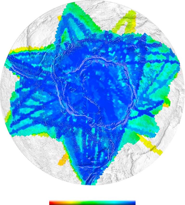
Journal of Geophysical Research: Solid Earth                                               10.1002/2014JB011332

                 SV velocity. The model of AN1-S fit our dispersion data better than CRUST2.0 + IASPEI91 in all periods,
                 particularly in periods of 150 s; we observed a mean variance reduction of 76% in fitting our
                 dispersion data in all periods relative to CRUST2.0 + IASPEI91.
                 For a strongly and laterally heterogeneous area, such as at the continent-ocean boundary, an S-velocity model
                 retrieved from surface wave dispersion can show general velocity variation trends in the vertical direction.
                 However, the detailed vertical variations of the determined velocities may be artificial [An and Assumpção,
                 2005, 2006]; consequently, we do not interpret the detailed structure just beneath continent-ocean transition
                 zones where the lateral structural variation may be marked over a short distance.
                 Moho depths and crustal thicknesses referred to below are the distance from the solid surface to the Moho.
                 We note that this definition of Moho depth is different from that in the compilation of AN-Moho (Table S1 in
                 the supporting information).

                 4.1. Three-Dimensional S-Velocity Structure Model
                 4.1.1. Representative 1-D Profiles
                 Figure 5 shows three examples of 1-D S-velocity profiles, which have been selected based on the new,
                 broad-scale models that we have derived. The three profiles are used as representative of significant regions
                 beneath EANT, WANT, and oceanic parts of the Antarctic Plate, respectively.
                 Figure 5a is a representative profile beneath the GSM, EANT. An S velocity of lower than 2 km/s in the top
                 layer (Figure 5a) represents ice covering in Antarctica. At depths of 40–70 km, the inverted seismic
                 velocities are obviously lower than the upper mantle velocities from IASPEI91 (the upper mantle velocities
                 in the initial reference model). If 4.2 km/s is taken as the velocity at the Moho, then the Moho is ~60 km
                 deep in the 1-D profile, which is clearly larger than ~40 km deep from the CRUST2.0 model (the crust
                 thickness in the initial reference model), indicating a very thick crust beneath the GSM, in agreement with
                 recent studies [Hansen et al., 2010; Heeszel et al., 2013; Feng et al., 2014]. At depths of 200–250 km, S-velocities
                 decrease downward with depth, which indicates that the top of the seismic low-velocity zone (LVZ), also
                 called seismic lithosphere-asthenosphere boundary, is at a depth of greater than 200 km.
                 Figure 5b shows a profile in WANT in the region of the West Antarctic rift system (WARS). In this region, the
                 crust is thin and ~25 km thick. Upper mantle S velocities decrease with depth at depths of ~80–110 km,
                 indicating that the upper bound of the seismic LVZ is no deeper than 100 km.
                 Figure 5c is a representative profile beneath an oceanic region where the crust is very thin (
Journal of Geophysical Research: Solid Earth 10.1002/2014JB011332
a) b)
c) d)
Figure 6. S-velocity maps at depths of (a) 30 km, (b) 100 km, (c) 150 km, and (d) 200 km. The symbols and labels are the
same as in Figure 1.
deeper structure beneath this region. However, the anomaly patterns of the low velocities should be true
because the half extents of the anomalies are close to or longer than the resolution lengths (Figures S3 and S4
in the supporting information) of our model at the these depths (100, 150, and 200 km). Furthermore, the
extremely low velocities in Figure 6c in our model are mostly beneath hot spots, such as Balleny hot spot (Bal),
Marion hot spot (Mar), and Bouvet hot spot (Bou), beneath which an extremely low velocity in the
asthenosphere is expected, suggesting that these low-velocity values in our model are reasonable.
At a depth of 100 km (Figure 6b), all of the Antarctic Plate is in the upper mantle; however, some regions are in
the lithosphere and some are in the asthenosphere. According to the lithosphere thicknesses implied from
the 1-D profiles in Figure 5, EANT at the depth of 100 km is still in the high-velocity seismic lid (or seismic
lithospheric upper mantle), whereas for WANT, 100 km depth represents the base of the lithosphere and for
oceanic regions, 100 km depth is in the asthenosphere. In oceanic regions from 0°E and 140°E, there is a
high-velocity zone relative to the other oceanic regions, particularly beneath the area from 20°E and 100°E,
where the velocities are similar to those beneath EANT.
AN ET AL. ©2014. American Geophysical Union. All Rights Reserved. 368Journal of Geophysical Research: Solid Earth 10.1002/2014JB011332
(a) (d)
(b)
(c)
Figure 7. Representative S-velocity vertical transects. The transects (a–d) cross the South Pole, (e–g) cross the GAMSEIS array, and (h–j) are along latitudes of 70°S, 75°S,
and 80°S, respectively. Transect A-A′ (Figure 7a) crosses the South Pole, GSM, and the St. Paul–Amsterdam hot spot (STP). Transect B-B′ (Figure 7b) crosses WANT,
South Pole, and EANT. Transects L-L′ (Figure 7e) and M-M′ (Figure 7f ) cross the TAM and GSM, respectively. Transect N-N′ (Figure 7g) crosses Domes A and C.
All transect positions are shown in the inset plot, in which shading is the Antarctic bedrock surface from Bedmap2 [Fretwell et al., 2013] and in other areas is the
surface topography from ETOPO2. For each transect, the black and gray shaded areas indicate the continental and oceanic exaggerated topography, respectively.
The black dots with error bars beneath the inverted blue-filled triangles mark the Moho positions from AN-Moho. All the inverted white-filled triangles and most
of the blue-filled triangles are seismic stations used in this study. Earthquakes shown are from 1900 to 2007 taken from the EHB catalog [Engdahl et al., 1998].
The black dots mark the 4.2 km/s isovelocity contour of the inverted solution. KP = Kerguelen Plateau, SP = South Pole, and ZhS = Zhongshan. The others are the
same or from the same sources as in Figure 1. The circles labeled with U mark the positions that the 4.2 km/s isovelocity contour is too deep.
In Figure 6d, the 200 km deep map still shows high velocities (>4.5 km/s) beneath parts of East Antarctica,
demonstrating that the continental lithosphere extends deeper than 200 km. In detail, the highest velocities
can be found at the large region from the GSM (Dome A) to Dome C (Figure 6d), beneath which thickest
lithospheres of the Antarctic Plate should be located.
4.1.3. Representative Vertical Transects
Ten representative S-velocity transects are shown in Figure 7. Transects from A-A′ to D-D′ in Figures 7a–7d
cross the South Pole; transections L-L′, M-M′, and N-N′ in Figures 7e–7g are aligned with the TransAntarctic
Mountains Seismic Experiment (TAMSEIS) and GAMSEIS arrays; and transections 7-7′, 1-1′, and 8-8′ in
Figure 7h–7j are along latitudes of 70°S, 75°S, and 80°S, respectively. The TAMSEIS and GAMSEIS projects
deployed linear arrays across the Transantarctic Mountains (TAM) and the GSM. All of the data obtained in
these two projects were used in this study, and therefore, the four transects (A-A′, L-L′, M-M′, and N-N′) in
Figure 7 have good resolution due to the proximity of the seismic stations.
As pointed out previously, a velocity of 4.2 km/s can be taken as preliminary indicator of the Moho. While this
definition may be arbitrary, Moho depths in the compilation of previous Moho determinations (AN-Moho)
can be used as a reference to evaluate if the Moho topography corresponds to the isovelocity contour in our
model. Given this, we have annotated the Moho from AN-Moho, along with the 4.2 km/s isovelocity contour,
in the transects shown in Figure 7. Before comparing Moho depths (mostly derived from receiver functions)
AN ET AL. ©2014. American Geophysical Union. All Rights Reserved. 369Journal of Geophysical Research: Solid Earth 10.1002/2014JB011332
(e) (h)
(f) (i)
(g) (j)
Figure 7. (continued)
with the isovelocity contour from surface waves, we note that they, in part, measure different features: the
results from receiver function analysis only represent the local structure beneath the station, however, those
from surface wave inversions, as in our model, average information over a large lateral area.
Transect A-A′ (Figure 7a) covers the Chinese traverse from Dome A to Zhongshan station (ZhS) (inset map in
Figure 7) and not only crosses the South Pole and the central regions of WANT (e.g., WARS) and EANT
(e.g., GSM) but also a range of oceanic tectonic areas (e.g., normal oceanic lithosphere, the submarine plateau
of Kerguelen large igneous province, and mid-ocean ridges) as well as volcanoes in WANT and the St.
Paul–Amsterdam hot spot (STP). This transect is the most extensive across the Antarctic Plate. The 4.2 km/s
isovelocity contour beneath five stations (CHNB, EAGLE, DT154, Zhongshan, and DAVI) to the north of the
GSM is shallower than the Moho depths in AN-Moho. The five stations are located near the border of Princess
Elizabeth Land and close to the Lambert Graben valley. The inconsistency of the isovelocity contour with
Moho depths for these stations indicates that the crustal structure beneath this region may be different as
compared with other regions of continental Antarctica and therefore requires a higher velocity definition of
the Moho beneath this region. Apart from these five stations, the contour line is consistent with the Moho
positions from AN-Moho, including the shallow Moho beneath WANT and the deep Moho just beneath the
GSM. The consistency indicates that a 4.2 km/s contour defines Moho topography for at least most of the
continental region. In the oceanic region of the transect, although the resolution of our model is low, the
model still shows some details of Moho variations, such as thicker crust just beneath the Kerguelen submarine
plateau (KP) than in the other oceanic regions. At the depths of 80–250 km, S velocities beneath East Antarctica
is higher than other regions, indicating that the base of seismic lid beneath EANT, particularly beneath the GSM,
can be at the depths of >200 km.
In addition to also crossing a mid-ocean ridge, oceanic lithosphere, and EANT, transect B-B′ is a representative
transect crossing the TAM and WARS of WANT. The contour is abruptly too deep at two positions labeled “U”
in the figure. At the two positions, a velocity of 4.2 km/s may be too high to represent the Moho, which
AN ET AL. ©2014. American Geophysical Union. All Rights Reserved. 370Journal of Geophysical Research: Solid Earth 10.1002/2014JB011332
implies a lower velocity at the Moho at
these two positions. The 4.2 km/s
isovelocity contour (Figure 7b) closely
coincides with the Moho beneath the
station in WARS.
Transect L-L′ is along the station arrays of
GAMSEIS and TAMSEIS and should have
highest resolution at positions beneath
the stations. Transect M-M′ is nearly
parallel to and along a similar region as
L-L′. Transect N-N′ crosses EANT and,
notably, Dome A in the GSM and Dome C.
Crust that is markedly thicker than
neighboring areas is found beneath
Dome A in the GSM in transects L-L′ and
N-N′. The 4.2 km/s isovelocity contour
line of transects L-L′, M-M′, and N-N′
(Figures 7e–7g) is consistent with the
position of the Moho discontinuity in
AN-Moho beneath most of the seismic
stations. In transects M-M′ and N-N′, the
Figure 8. Depth map of isovelocity contours for S velocity at 4.2 km/s. isovelocity contour at a position labeled U
The circles labeled with U mark the positions that the 4.2 km/s abruptly deepens, which requires a lower
isovelocity contour is too deep. Moho velocity just at the positions.
In summary, the above figures provide good definition of the lithosphere and asthenosphere beneath
Antarctica. EANT has a thick crust and lithosphere, with the thickest crust probably beneath the GSM, but the
thickest lithosphere (>200 km) most likely occurs between Dome A and Dome C. The oceanic region has
thinnest crust and lithosphere. WANT has an intermediate crust and lithosphere between EANT and oceanic
region. Furthermore, the 4.2 km/s isovelocity contour line closely coincides with the Moho discontinuity from
most data in AN-Moho, including beneath intracontinental seismic stations and some stations close to the
Figure 9. Crustal thickness (Moho discontinuity) map of the Antarctic Plate. The symbols are the same as those in Figure 1.
AN ET AL. ©2014. American Geophysical Union. All Rights Reserved. 371Journal of Geophysical Research: Solid Earth 10.1002/2014JB011332
continent-ocean transition zone. This
a) indicates that the Moho discontinuity
topography can be depicted by the
isovelocity contour obtained from our 3-D
S-velocity model in most areas.
4.2. Moho Topography
4.2.1. Construction of AN1-CRUST
Our S-velocity transects indicate that the
4.2 km/s isovelocity contour corresponds
with most of the Moho depths estimated
from previous body wave studies. The
4.2 km/s S-velocity contour topography is
shown in Figure 8. However, as described
above, at areas marked with circles labeled
U in Figure 8 and in vertical transects M-M′,
b) N-N′, and B-B′ (Figure 7), the S-velocity
contour of 4.2 km/s is unusually deep.
These areas have a lower velocity at the
top of the upper mantle relative to
neighboring regions. Therefore, the
velocity at the Moho is somewhat variable
throughout Antarctica.
In order to evaluate the S velocities in the
vicinity of the Moho (VMoho), we retrieved
S velocities at all the Moho depths in
the compilation of AN-Moho from our
S-velocity model, AN1-S. The mean of all
the S velocities at the Moho is 4.21 km/s
with a standard deviation of 0.28 km/s.
This confirms the correspondence of the
position with an S velocity of 4.2 km/s to
almost the Moho depths but also
indicates that VMoho is not fixed but has
significant variability.
Figure 10. Relationship between crustal thicknesses in AN1-CRUST,
Using equation (3) and considering the
derived from 3-D S-velocity model of AN1-S, and the constraints in
range of S velocities, which are possible at
AN-Moho, from previous studies. (a) The error bars represent the
the Moho described above, we retrieved a
uncertainty (5 km) for each Moho point because of the 5 km layer
map of the Moho topography (or crustal
thickness in our 3-D S-velocity model around the Moho. The red plus
symbols are the average crustal thickness in AN1-CRUST in each thickness) from our 3-D seismic model,
interval of 4 km. (b) The plate shows the geographical distribution of
which we denote as AN1-CRUST (Figure 9).
the differences (circles) between the two data sets illustrated in
Given that Rayleigh waves with an average
Figure 10a. The blue circles indicate where the thickness in AN-Moho
period of 50 s can resolve the structure
is more than that of AN1-CRUST, whereas the red circles indicate
where the opposite is the case. down to ~50 km and that the Moho depth
of the Antarctic Plate is less than 65 km
everywhere, the resolution map of 50 s shown in Figure S3c in the supporting information indicatively
represents the lateral resolution length of the Moho topography.
The correlation between the Moho depths in AN1-CRUST and AN-Moho are shown in Figure 10a, and the
geographical distribution of the differences between the two data sets is shown in Figure 10b. A good
correlation generally exists between the average Moho depths (red plus symbols in Figure 10a) from
AN1-CRUST and AN-Moho, mostly in Antarctic continent. Besides in the continent, the Moho depths in the
oceanic region (Figure 9) determined from AN1-S using equation (3) are still reasonable, which demonstrates
that the definition of the Moho position in equation (3) can be simultaneously used in various regions. Most
AN ET AL. ©2014. American Geophysical Union. All Rights Reserved. 372Journal of Geophysical Research: Solid Earth 10.1002/2014JB011332
of the points with a large difference between the two data sets are near tectonic transition zones, such as
continent-ocean transitions (Figure 10b), where complex and large lateral variations in Moho topography
may occur over short distances that are not resolvable with our model.
4.2.2. Main Features of the Antarctic Crustal Thickness Map
The TAM divides Antarctica into two blocks (EANT and WANT) with distinctly different crustal thicknesses.
The whole of EANT has crust thicker than 40 km, and the thickest crust (~61 km) in Antarctica is located
just beneath Dome A, at the center of the GSM. The areas close to QML and Dome F, where no reliable
information on the crust was previously available, also has thick crust similar to that of the GSM. Therefore,
the topographic highs of the EANT Mountain Ranges (EAMOR or called EANT Highlands) from QML to Dome F
and then to the GSM (Figure 1) are all underlain by thick crust (zoom-in inset of Figure 9). The Lambert Graben
area, including the Amery ice shelf, has relatively thin crust, which is another pronounced feature of EANT.
In WANT, the southern boundary, close to the regions form TAM to Ellsworth Land (ElL), of the WARS
separates WANT into two blocks with markedly different crustal thicknesses. The crust beneath the WARS is
thin, and the Ross Sea area beneath the Ross ice shelf (RIS) has the thinnest crust in Antarctica (Figures 7j and 9).
The crust is somewhat thicker in Marie Byrd Land and along the East (Siple) coast of the Ross Sea. Most of the
other regions in WANT, including the Ronne ice shelf (rIS), have similar crustal thicknesses that are more than
30 km. Interestingly, the northern tip of the Antarctic Peninsula has crust that is thicker than in surrounding
areas, which will be discussed in M. An et al. (manuscript in preparation, 2014).
As we expected, the oceanic crust is generally thin, except for a thicker crust just beneath the Kerguelen
submarine plateau. However, we note that the resolution of our model in the oceanic region is poor.
5. Discussion
5.1. Comparison of AN1-CRUST With Other Recent Models
The oceanic crust is generally thin (Journal of Geophysical Research: Solid Earth 10.1002/2014JB011332
topography. For example, the highlands
of the EAMOR region corresponds to a
negative depression of the Moho
discontinuity and, beneath the highest
point (Dome A of the GSM), the Moho
discontinuity is at its deepest point. This
relationship indicates that East Antarctica
is largely isostatically compensated
according to an Airy isostasy model.
5.2.1. Crustal Density-Thickness
Relationships From an Airy
Isostasy Model
According to the Airy-Heiskanen isostasy
Figure 11. Crustal thickness as a function of surface elevations. The model [Airy, 1855; Heiskanen, 1931], crustal
elevation at any point in this figure was corrected for ice and water
thickness can be assumed to have a linear
layers by adding an equivalent rock thickness with the same mass as
the ice and water to the rock surface. The densities of water, ice, and relationship with surface elevation, for
3
rock used in the conversion are 1, 0.92, and 2.8 Mg/m , respectively. assumed average crustal (ρc) and upper
The lines are linear fits of crustal thicknesses and elevations. The surface mantle (ρm) densities. If water of thickness
elevation data were taken from ETOPO2, and the ice thickness data
(hw) (ρw = 1.0 Mg/m3) and ice of thickness
were taken from Bedmap2 [Fretwell et al., 2013].
(hi) (ρi = 0.92 Mg/m3) are also considered,
then the surface topography will be the sum of hi, hw, and the rock surface elevation. After surface elevation is
corrected by converting hi and hw to equivalent rock thicknesses, the Airy isostasy model is represented by the
linear relationship between corrected surface elevation (hc) and crustal thickness (H) as follows:
ρc 1
H ¼ H0 þ hc ¼ H0 þ hc ; (4)
ρm ρc ρm =ρc 1
where H0 is a constant representing zero-elevation crustal thickness. If two more groups of H and hc are
known, H0 and ρm/ρc can be estimated from equation (4).
Using AN1-CRUST and AN-Moho, crustal thicknesses as a function of topographic elevations for the Antarctic
continent are shown in Figure 11. The parameters H0 (vertical intercept) and ρm/ρc (related with slop) for the
linear relationship (equation (4)) are marked in the figure. The linear relationship of Antarctica is very different
with that in the average of other continents, as demonstrated below.
In global continental areas with a crustal thickness of >30 km, the topography at 0 km is found to correspond
to a zero-elevation crustal thickness (H0) of 40 km [Watts, 2007], based on the Airy model and using the global
crustal model of CRUST2.0 [Bassin et al., 2000]. However, for Antarctica, if only using the crustal thicknesses
from AN-Moho, then H0 is ~28 km (Figure 11), and all crustal thicknesses from AN1-CRUST in the Antarctic
continent give a value of H0 of ~30 km. Similar result can be found if only the regions with a crustal thickness
of >30 km in the Antarctic continent are considered (Figure 11). Thus, the H0 (~30) for Antarctica is markedly
smaller that for the global average (40 km).
5.2.2. Densities Inferred From Airy Isostasy
The average oceanic crustal density is 2.89–3.00 Mg/m3 [Carlson and Raskin, 1984], and the average
continental crust density is 2.83 Mg/m3 [Christensen and Mooney, 1995]. Using ρm = 3.30 Mg/m3 suggested by
Wang [1970] and considering the ratios (ρm/ρc) (Figure 11) from AN-Moho and AN1-CRUST, the estimated
average crustal densities for the Antarctic continent would be ~3.0 and ~2.94 Mg/m3. These calculated
average crustal densities are close to the upper range of average oceanic crust and are ~0.1 Mg/m3 higher than
the typical density (2.83 Mg/m3) of continental crust. In general, if a thermal expansion value of 3.0 × 10⁵ K1
for the crust is used, a 100° temperature variation can cause a ~0.01 Mg/m3 density variation for a mineral with a
density of 2.9 Mg/m3 [Tassara, 2006]. Therefore, a density increase of 0.1 Mg/m3 requires a temperature drop of
~1000°, which is unrealistically large to explain the above calculated average crustal densities for the Antarctic.
Therefore, the density ratios (ρm/ρc) given by linear relationship (Figure 11) are anomalously small.
Another possibility which results in the anomalous low density ratio is that the mantle density ρm is much
smaller than 3.30 Mg/m3 that we used. In general, the density in subcontinental lithospheric mantle (SCLM)
AN ET AL. ©2014. American Geophysical Union. All Rights Reserved. 374Journal of Geophysical Research: Solid Earth 10.1002/2014JB011332
may be related with its age (e.g., in Archean
a)
(3.31 ± 0.016 Mg/m3) < Proterozoic
(3.35 ± 0.02 Mg/m3) < Phanerozoic
(3.36 ± 0.02 Mg/m3))[Poudjom Djomani
et al., 2001]. The lithospheric mantle
density of 500 km) topography of the Earth’s surface is generally due to variations in crustal
thickness in combination with the large-density contrast between crust and mantle [Cazenave, 1995;
Turcotte and Schubert, 2002]. Therefore, we focus on the large-scale anomalies in Figure 12. From the
anomaly patterns in the two maps (Figures 12a and 12b), Antarctica can be divided into several regions,
as below.
AN ET AL. ©2014. American Geophysical Union. All Rights Reserved. 375Journal of Geophysical Research: Solid Earth 10.1002/2014JB011332
Three large regions (Figure 12b) have negative values of ΔH: the block labeled by “SAF” that was once
connected with the South American and African continents, which is located from 20°W to 60°W and includes
the Weddell Sea and Ronne ice shelf; the block labeled by “AUR,” that was once connected with the Australian
continent, located from 100°E to 155°E; and the Lambert Graben region which is a Permian Rift. These
negative values correspond to relatively high average crustal density or low SCLM density. Given that
Antarctica generally has a smaller ρm/ρc than other continents, as shown above, the negative anomaly of
these regions is an unusual feature. Archean rocks found in George V Land (142°02′E–153°45′E) and Terre
Adélie (136°E–142°E) of AUR [Fanning et al., 1988; Flöttmann and Oliver, 1994; Boger, 2011] suggest that the
lithosphere of the AUR block is Archean and the SCLM is lighter and more bouyant.
The SAF region and Lambert Graben also show negative values (Figure 12); however, the values cannot be
attributed to low SCLM density or old SCLM because these regions are not as old as AUR blocks and even
younger than EAMOR. The negative values in SAF and the Lambert Graben may imply a high density of the
cooled crust which was intruded by mafic melts associated with magmatism during rifting in Permian
[Harrowfield et al., 2005].
The positive values of ΔH in WARS (Figure 12a) may be due to thermal effects. The WARS is a major active
continental rift associated with late Oligocene to recent volcanic activity [Behrendt et al., 1991], and
thermal isostasy may affect some continental regions such as continental rifts, back arcs, and regions
characterized by extensive volcanism [Hasterok and Chapman, 2007]. Besides, most of the mountain ranges
have positive anomalies (Figure 12b), such as the TAM and EAMOR (e.g., the mountains close to and north
of Dome F). The positive anomaly beneath the TAM may reflect Cenozoic thermal or other dynamic effects
[ten Brink et al., 1997; Hamilton et al., 2001; Studinger et al., 2004; Bialas et al., 2007; Faure and Mensing, 2010];
e.g., asthenosphere upwelling and intrusion into SCLM can result in the increase of upper mantle density
and the increase of crustal temperature which can resulted in the decrease of crustal density. However, in
EAMOR, the anomaly cannot be attributed to Cenozoic tectonism, as no such activity has taken place since
the Cambrian.
5.3. Do the EAMOR Represent a Gondwanan Suture?
Obscured beneath a thick ice cap, the elevated (>3 km) and rugged relief of the GSM, part of EAMOR, has
long been considered enigmatic and was key research target as part of the Fourth IPY. Recent measurements
[e.g., Hansen et al., 2010; Heeszel et al., 2013; Feng et al., 2014] and this study have found a very thick crust
(~60 km) beneath the GSM, the topographic high of Antarctica. In the upmost upper mantle, similar to
that found in the GSM by previous Rayleigh wave study [Heeszel et al., 2013], our results showed that the
continental seismic lithosphere of the GSM extends deeper than 200 km. Temperature analyses in a later
paper of M. An et al. (manuscript in preparation, 2014) demonstrated that thermal lithosphere beneath the
GSM is also >200 km thick. Therefore, the striking features of the GSM are its high elevation, very thick crust
(~60 km), and lithosphere (>200 km). This study shows that similar features of thick crust and lithosphere
extend across the entire EAMOR region. Given these similarities, the crusts beneath the EAMOR should be
formed with similar tectonic events and in the similar time.
Within the framework of global tectonic evolution, several models have been proposed to explain the
formation of the GSM. Thermal effects can generate topographic highs. It has been suggested that the GSM
resulted from a Cenozoic (approximatelyJournal of Geophysical Research: Solid Earth 10.1002/2014JB011332
Vs (km/s)
Globally, horizontal shortening at the present compressional
2 3 4 5
0 orogenic regions can result in the above features (high
topography, thick crust, and lithosphere) of the GSM.
Fo example, the subduction of continental or oceanic plates
underlying a large continent can result in both a topographic
50 high and very thick crust in the Alpine-Himalayan
mountain ranges [Hirn et al., 1984; Zhao et al., 1993;
Hauck et al., 1998] and the Andes [Beck et al., 1996; Yuan
et al., 2002; Assumpção et al., 2013]. The lithosphere
100
can also thicken under compression to produce a very
Depth (km)
thick lithosphere such as in the Himalayas [An and Shi,
2006; Feng and An, 2010; Feng et al., 2010] and Andes
[Feng et al., 2004, 2007].
150
In order to check the similarities between the lithosphere
structures, we compared the S velocities beneath the
GSM with those of present orogenies (the Andes and the
200 Himalayas) and a Proterozoic convergent orogeny
(the Grenville) (Figure 13). The Grenville orogeny took
Grenville model
Himalayan model
place at 1.0–1.3 Ga [Tollo et al., 2004]. The figure shows
Andean model that the S-velocity variation beneath the GSM is similar
250 GSM model
to those beneath the present orogenies down to the
depth of 140 km (Figure 13). The Andean model matches
Figure 13. Comparison of S velocities beneath the the GSM model well throughout the profile, but the
GSM with those in other continents. The model Himalayan model lacks the high-velocity lithosphere at
beneath the GSM is the same as that in Figure 5a. The
depths greater than 150 km. The GSM model is similar to
Andean model is of the S velocities at the point (68°W,
21°S) from Feng et al. [2004], and the Himalayan that of the Grenville model in the crust down to 30 km;
model is at the point (89°E, 28°N) from Feng and An however, marked difference can be found in the depths of
[2010]. The Andean and Himalayan models were 30–170 km. These similarities with present convergent
inverted from similar data (Rayleigh wave group orogenies confirm the viewpoint that the GSM was formed
velocities) by similar inversion methods to that for the
GSM. The Grenville model is at the point (76°E, 46°N)
during a convergent (subduction or collision) orogeny.
in Middle Proterozoic Grenville orogen of the North It has been proposed that the GSM formed in response to
American craton inverted from Rayleigh wave group/
late Carboniferous-Early Permian (~300 Ma) far-field
phase velocities by two-step ray-based tomography
[Shapiro and Ritzwoller, 2002]. compression associated with the formation of Pangaea
[Veevers, 1994; Veevers et al., 2008]. While a compressional
orogen can generate a plateau or a mountain range,
such as the Tibetan Plateau or the Andes, in the near-field of the compression zone, mountain ranges are
seldom generated in the far field. Studies on Detrital zircons from coastal parts of EANT show no zircons of
Carboniferous age [van de Flierdt et al., 2008; Veevers and Saeed, 2011]. Consequently, it is unlikely that the
GSM formed with the formation of Pangaea.
The pre-Cenozoic orogenic belts in EANT developed during four major orogenic cycles [Talarico and
Kleinschmidt, 2008] spanning approximately 0.9–1.3 Ga (Grenvillian-aged orogens), 500–600 Ma (Ross and
Pan-African orogens), 200–250 Ma (Ellsworth or Weddell Orogen), and 90–150 Ma (Antarctic Andean
Orogen), with only the Grenvillian- and Pan-African-aged orogens occurring anywhere near the GSM.
The GSM lies near the Grenvillian-aged Payner orogen and may have also formed in Grenvillian time.
However, the crust of the EAMOR was distributed across several continents prior to the formation of
Gondwana and cannot have formed from a Grenvillian-aged orogeny during the amalgamation of the
Rodinia supercontinent. The marked difference between the GSM and Grenville S-velocity structures
(Figure 13) also suggests that the GSM was not formed by a Grenvillian-aged orogen. Consequently, the
GSM must have formed in response to Late Neoproterozoic (500 Ma) orogenic activities associated with the assembly of Gondwana, which is compatible with
geological evidence [Zhao et al., 1995; Fitzsimons, 2000, 2003; Liu et al., 2003, 2006] found close to the
continent margins of EANT.
AN ET AL. ©2014. American Geophysical Union. All Rights Reserved. 377Journal of Geophysical Research: Solid Earth 10.1002/2014JB011332
Figure 14. Comparison of interpretation with lithospheric upper mantle S-velocities at the depth of 200 km and crustal
thicknesses. The former is the same as in Figure 6d and the latter as in Figure 9. The symbols and labels are the same as
in Figure 1 or Figure 12b.
Before 550 Ma, the GSM may have been part of East Gondwana (Figure S1 in the supporting information),
which consisted of Australia and most of EANT, while the north Prince Charles Mountains and India belonged
to Indo-Antarctica which amalgamated with West Gondwana prior to 550 Ma [Boger et al., 2002; Boger, 2011].
East Gondwana amalgamated with the large continent composed of West Gondwana and Indo-Antarctica
after 550 Ma (Figure S1 in the supporting information and Figure 15b), and as such, the GSM should lie close
to the suture. We observe that the S-velocity variation in the upper mantle beneath the GSM is more similar
to that observed beneath the Andes than the Himalayas (Figure 5), indicating that the GSM is formed by
an oceanic subduction like in the Andes. However, no oceanic plate can be found adjacent to the GSM after
Gondwana amalgamated; therefore, the GSM should be intermediate orogeny between the Andes and
Himalayas; i.e., the GSM formed by oceanic subduction overlying a continent and the subduction finally
stopped after Gondwana supercontinent is amalgamated. Considering that the oceanic plate subduction in
South American only resulted in a large mountain chains (the Andes), while the continental subduction or
collision in the Himalayas produced a broad topographic high (the Tibetan Plateau), it is unlikely that a
plateau like the Tibetan Plateau was formed during the Gondwanan amalgamation.
Given the similarities in crustal thicknesses and surface topography across the EAMOR, including the
GSM and the mountains close to Dome F, the EAMOR may represent the convergent suture between
East Gondwana and the large continent of West Gondwana and Indo-Antarctica that formed during the
Pan-African orogen during 550–500 Ma, as illustrated in Figure 15. If the above processes are true, the
lithosphere beneath EAMOR would be formed and transformed just during the above tectonic events, and
as such, the lithosphere of EAMOR should be younger than neighboring regions. The analyses from Airy
isostasy in the last subsection indicated that the lithosphere of EAMOR is younger than the Archean
AUR and SAF, which supports the above hypothesis. However, a 500 Ma age for the EAMOR lithosphere is
generally incompatible with the very thick fast velocity lithosphere, which shows greatest similarity to early
Proterozoic and Archean regions worldwide [Heeszel et al., 2013]. One possibility is that the Pan-African
collisional orogeny that produced the GSM juxtaposed and thickened older lithosphere of the colliding
terraines.
A basic issue for a subduction is to discriminate which one of the convergent blocks were the overriding and
subducting blocks. Due to underlying subduction, respectively, by the Indian continent and Nazca Plate, the
Tibetan Plateau and the South American continent have thick lithosphere close to the subduction zone.
AN ET AL. ©2014. American Geophysical Union. All Rights Reserved. 378You can also read