Simulation of reactive solute transport in the critical zone: a Lagrangian model for transient flow and preferential transport - HESS
←
→
Page content transcription
If your browser does not render page correctly, please read the page content below
Hydrol. Earth Syst. Sci., 25, 1483–1508, 2021
https://doi.org/10.5194/hess-25-1483-2021
© Author(s) 2021. This work is distributed under
the Creative Commons Attribution 4.0 License.

Simulation of reactive solute transport in the critical zone:
a Lagrangian model for transient flow and
preferential transport
Alexander Sternagel1 , Ralf Loritz1 , Julian Klaus2 , Brian Berkowitz3 , and Erwin Zehe1
1 KarlsruheInstitute of Technology (KIT), Institute of Water Resources and River Basin Management,
Hydrology, Karlsruhe, Germany
2 Luxembourg Institute of Science and Technology (LIST), Environmental Research and Innovation Department,

Catchment and Eco-Hydrology Research Group, Esch-sur-Alzette, Luxembourg
3 Department of Earth and Planetary Sciences, Weizmann Institute of Science, Rehovot, Israel

Correspondence: Alexander Sternagel (alexander.sternagel@kit.edu)

Received: 12 October 2020 – Discussion started: 21 October 2020
Revised: 22 February 2021 – Accepted: 23 February 2021 – Published: 25 March 2021

Abstract. We present a method to simulate fluid flow with re-      cope with preferential bypassing of topsoil and subsequent
active solute transport in structured, partially saturated soils   re-infiltration into the subsoil matrix.
using a Lagrangian perspective. In this context, we extend
the scope of the Lagrangian Soil Water and Solute Trans-
port Model (LAST) (Sternagel et al., 2019) by implement-
ing vertically variable, non-linear sorption and first-order       1   Introduction
degradation processes during transport of reactive substances
through a partially saturated soil matrix and macropores.          Reactive substances like pesticides are subject to chemi-
For sorption, we develop an explicit mass transfer approach        cal reactions within the critical zone (Kutílek and Nielsen,
based on Freundlich isotherms because the common method            1994; Fomsgaard, 1995). Their mobility and life span de-
of using a retardation factor is not applicable in the particle-   pend greatly on various factors like (i) the spectrum of trans-
based approach of LAST. The reactive transport method is           port velocities, (ii) the sorption to soil materials (Knabner et
tested against data of plot- and field-scale irrigation experi-    al., 1996), and (iii) microbial degradation and turnover (cf.
ments with the herbicides isoproturon and flufenacet at dif-       Sect. 3). The multitude and complexity of these factors are
ferent flow conditions over various periods. Simulations with      a considerable source of uncertainty in pesticide fate mod-
HYDRUS 1-D serve as an additional benchmark. At the plot           elling. It is still not fully understood how pesticides are trans-
scale, both models show equal performance at a matrix-flow-        ported within different soils and particularly how preferential
dominated site, but LAST better matches indicators of prefer-      flow through macropores impacts the breakthrough of these
ential flow at a macropore-flow-dominated site. Furthermore,       substances into streams and groundwater (e.g. Flury, 1996;
LAST successfully simulates the effects of adsorption and          Arias-Estévez et al., 2008; Frey et al., 2009; Klaus et al.,
degradation on the breakthrough behaviour of flufenacet with       2014).
preferential leaching and remobilization. The results demon-          To advance our understanding of reactive solute transport
strate the feasibility of the method to simulate reactive so-      (RT) of pesticides, particularly the joint controls of macrop-
lute transport in a Lagrangian framework and highlight the         ores, sorption, and degradation, a combination of predictive
advantage of the particle-based approach and the structural        models and plot-scale experiments is often used (e.g. Zehe
macropore domain to simulate solute transport as well as to        et al., 2001; Simunek et al., 2008; Radcliffe and Simunek,
                                                                   2010; Klaus and Zehe, 2011; Klaus et al., 2013). Such meth-
                                                                   ods allow for the assessment of the environmental risks aris-

Published by Copernicus Publications on behalf of the European Geosciences Union.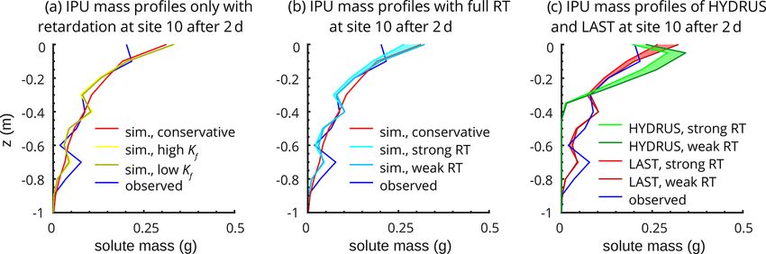
1484                                          A. Sternagel et al.: Simulation of reactive solute transport in the critical zone

ing from the wide use of reactive substances (Pimentel et al.,     rally changing soil moisture states and boundary conditions.
1992; Carter, 2000; Gill and Garg, 2014; Liess et al., 1999).      This explains why only a relatively small number of models
Combining the Richards and advection–dispersion equations          use Lagrangian approaches for solute transport and also for
is one common approach used to simulate water flow dy-             water particles (also called water “parcels”) to characterize
namics and (reactive) solute transport in the partially satu-      the fluid phase itself (e.g. Ewen, 1996a, b; Bücker-Gittel et
rated soil zone. This approach has been implemented, for           al., 2003; Davies and Beven, 2012; Zehe and Jackisch, 2016;
example, in the well-established models HYDRUS (Gerke              Jackisch and Zehe, 2018). Sternagel et al. (2019) proposed
and van Genuchten, 1993; Simunek et al., 2008), MACRO              that these water particles may optionally carry variable solute
(Jarvis and Larsbo, 2012), and Zin AgriTra (Gassmann et            masses to simulate non-reactive transport. Their Lagrangian
al., 2013). However, this approach has well-known deficien-        Soil Water and Solute Transport Model (LAST) combines
cies in simulating preferential macropore flow and imperfect       the assets of the Lagrangian approach with an Euler grid to
mixing with the matrix in the vadose zone (Beven and Ger-          simulate fluid motion and solute transport in heterogeneous,
mann, 2013). As both processes essentially control environ-        partially saturated 1-D soil domains. It allows discrete water
mental risk due to transport of reactive substances, a range       particles to travel at different velocities and carry temporally
of adaptions has been proposed to improve this deficiency          variable solute masses through the subsurface domain. The
(Šimůnek et al., 2003). One frequently used adaption is the       soil domain is subdivided into a soil matrix and a structurally
dual-domain concept, which describes matrix and macrop-            defined preferential flow/macropore domain (cf. Sect. 2). A
ore flow in separated, exchanging continua to account for lo-      comparison of HYDRUS 1-D and the LAST-Model based on
cal disequilibrium conditions (Gerke, 2006). However, stud-        plot-scale tracer experiments showed that both models per-
ies show that even these dual-domain models can be insuf-          form similarly in the case of matrix-flow-dominated tracer
ficient to quantify preferential solute breakthrough into the      transport; however, under preferential flow conditions, LAST
subsoil (Sternagel et al., 2019) or into tile drains (Haws et      better matched observed tracer profiles, indicating preferen-
al., 2005; Köhne et al., 2009a, b). A different approach is to     tial flow (Sternagel et al., 2019).
represent macropores as spatially connected, highly perme-            While the results of Sternagel et al. (2019) demonstrate the
able flow paths in the same domain as the soil matrix (Sander      feasibility of the Lagrangian approach to simulate conserva-
and Gerke, 2009). This concept has been shown to operate           tive tracer transport, even under preferential flow conditions
well for preferential flow of water and bromide tracers at a       during 1 d simulations, a generalization of the Lagrangian ap-
forested hillslope (Wienhöfer and Zehe, 2014) and for bro-         proach to reactive solute transport and larger timescales is
mide and isoproturon transport through worm burrows into a         still missing.
tile drain at a field site (Klaus and Zehe, 2011). Neverthe-          The main objectives of this study are thus as follows:
less, this approach is based on the Richards equation and
is thus limited to laminar flow conditions with sufficiently        1. We develop a method for reactive transport, i.e. the sorp-
small flow velocities corresponding to a Reynolds number               tion and degradation of solutes within the Lagrangian
smaller than 10 (e.g. Bear, 2013; Loritz et al., 2017).                framework under well-mixed and preferential flow con-
   Particle-based approaches offer a promising alternative to          ditions, and implement this into the LAST-Model. We
simulate reactive transport. These approaches work with a              initially test the feasibility of the method by simulat-
Lagrangian perspective on the movement of solute parti-                ing plot-scale experiments with a bromide tracer and
cles in a flow field, rather than by solving the advection–            the herbicide isoproturon (IPU) during 2 d (Zehe and
dispersion equation directly. They have been particularly ef-          Flühler, 2001) and use corresponding simulations of the
fective in quantifying solute transport alone, while the move-         commonly applied model HYDRUS 1-D as a bench-
ment of the fluid carrying solutes is still usually integrated         mark.
in systems based on Eulerian control volumes (e.g. Delay
                                                                    2. We perform plot-scale simulations to explore the trans-
and Bodin, 2001; Zehe et al., 2001; Berkowitz et al., 2006;
                                                                       port behaviour of bromide and IPU with the Lagrangian
Koutsoyiannis, 2010; Klaus and Zehe, 2010; Wienhöfer and
                                                                       approach over 7 and 21 d to evaluate its performance on
Zehe, 2014). In the context of saturated flow in fractured
                                                                       longer timescales. For this purpose, we make use of data
and heterogeneous aquifers, Lagrangian descriptions of fluid
                                                                       from another plot-scale irrigation experiment (Klaus et
flow are already commonly and successfully applied. For ex-
                                                                       al., 2014).
ample, the continuous-time random walk (CTRW) approach
accounts for non-Fickian transport of tracer particles within       3. We conduct simulations of breakthrough experiments
the water flow through heterogeneous, geological formations            with flufenacet (FLU) on a tile-drain field site over a
via different flow paths with an associated distribution of ve-        period of 3 weeks (Klaus et al., 2014), to examine the
locities and thus travel times (Berkowitz et al., 2006, 2016;          breakthrough behaviour and remobilization of reactive
Hansen and Berkowitz, 2020). However, Lagrangian mod-                  substances.
elling of fluid flow in the vadose zone is more challenging
due to the dependence of the velocity field on the tempo-

Hydrol. Earth Syst. Sci., 25, 1483–1508, 2021                                       https://doi.org/10.5194/hess-25-1483-2021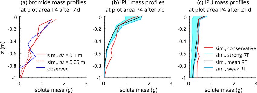
A. Sternagel et al.: Simulation of reactive solute transport in the critical zone                                                         1485

2     The LAST-Model: concept, theoretical background,              in good accord with simulations using a Richards equation
      and numerical implementation                                  solver. We refer the reader to the study of Zehe and Jack-
                                                                    isch (2016) for further details on the model concept.
2.1     Model concept
                                                                    Derivation of particle displacement equation
The LAST-Model combines a Lagrangian approach with an
Euler grid to simulate fluid motion and solute transport in         Our starting point is the soil-moisture-based form of the
heterogeneous, partially saturated 1-D soil domains. Discrete       Richards equation:
water particles with a constant water mass and volume carry         ∂θ    ∂K(θ )    ∂

                                                                                               ∂θ

temporally variable information about their position and so-           =         +       D (θ)      ,                     (1)
                                                                    ∂t      ∂z      ∂z         ∂z
lute concentrations through defined domains for soil matrix
and macropores that are subdivided into vertical grid ele-
                                                                    with D (θ ) = K (θ ) ∂9
                                                                                          ∂θ .
ments (Euler grid). Prior to simulation, the initial water con-
                                                                       By multiplying the hydraulic conductivity K in the first
tent of each grid element is converted to a corresponding wa-
                                                                    term of Eq. 1 by θθ (= 1), we obtain
ter mass with the grid element volume and water density. The
water mass of each grid element is summed to a total water          ∂θ

                                                                           ∂ K(θ )

                                                                                               ∂

                                                                                                          ∂θ

mass in the entire soil domain and then divided by the total            =              θ +         D (θ )      .           (2)
                                                                     ∂t    ∂z     θ          ∂z           ∂z
number of particles. In this way, the water particles in the soil
domain are initially defined by a certain water mass. During        Rewriting this equation leads to the divergence-based form
the simulation, the number of water particles is counted in         of the Richards equation:
each time step, and a new particle density per grid element
                                                                                                        ∂2

is computed. By multiplying this water particle density with        ∂θ      ∂ K(θ )       ∂D (θ )
                                                                        =             θ−          θ + 2 (D (θ) θ ) ,        (3)
the particle mass and water density, a new soil water con-          ∂t     ∂z     θ         ∂z         ∂z
tent per grid element and time step can be obtained (Zehe
and Jackisch, 2016). Different fractions of the water particles     where z is the vertical position (positively upward) in the soil
in a grid element correspond to the sub-scale distribution of       domain (m), K the hydraulic conductivity (m s−1 ), D the
the water content among soil pores of different sizes. Con-         water diffusivity (m2 s−1 ), 9 the matric potential (m), θ (t)
sequently, different water particle fractions travel at different   the soil water content (m3 m−3 ), and t the simulation time
velocities (cf. Fig. 1). Their displacements are determined by      (s).
the hydraulic conductivity and water diffusivity in combina-           Equation (3) is formally equivalent to the Fokker–Planck
tion with a spatial random walk (cf. Sect. 2.2, Eq. 5). This        equation (Risken, 1984). The first term of the equation corre-
approach accounts for the joint effects of gravity and cap-         sponds to a drift/advection term characterizing the advective
illary forces on water flow in partially saturated soils. The       downward velocity v (m s−1 ) of fluid fluxes driven by grav-
use of an Euler grid allows for the necessary updating of soil      ity:
water contents based on changing particle densities and re-
                                                                               K(θ ) ∂D (θ )
lated time-dependent changes in the velocity field. The space       −v (θ) =        −        .                                             (4)
domain approach also reflects the fact that spatial concentra-                  θ     ∂z
tion patterns and thus travel distances are usually observed        The second term of Eq. (3) represents diffusive fluxes driven
in the partially saturated zone. The Euler grid is hence nec-       by the soil moisture or matric potential gradient and con-
essary to calculate spatial concentration profiles and to prop-     trolled by diffusivity D(θ ) (cf. Eq. 1). Equation (3) can then
erly describe specific interactions between the matrix and the      be solved by a non-linear random walk of volumetric water
macropore domain.                                                   particles (Zehe and Jackisch, 2016). The non-linearity arises
                                                                    due to the dependence of K and D on soil moisture and hence
2.2     Underlying theory and model equations                       the particle density. The vertical displacement of water parti-
                                                                    cles is described by the Langevin equation:
2.2.1    Transient fluid flow in the partially saturated
         zone                                                                                    K (θr + i · 1θ ) ∂D (θr + i · 1θ )
                                                                    zi (t + 1t) = zi (t) −                       +
                                                                                                      θ (t)              ∂z
The LAST-Model (Sternagel et al., 2019) is based on the La-
                                                                                           p
                                                                                · 1t + Z 2 · D (θr + i · 1θ ) · 1t
grangian approach of Zehe and Jackisch (2016), which was                       i = 1, . . ., NB ,                                          (5)
introduced to simulate infiltration and soil water dynamics in
the partially saturated zone using a non-linear random walk         where the second term describes downward advection/drift
in the space domain. The results of test simulations con-           of water particles driven by gravity on the basis of the hy-
firmed the ability of the Lagrangian approach to simulate wa-       draulic conductivity K (m s−1 ). The term ∂D(θr∂z     +i·1θ)
                                                                                                                                  cor-
ter dynamics under well-mixed conditions in different soils,        rects this drift term for the case of spatially variable diffusion

https://doi.org/10.5194/hess-25-1483-2021                                         Hydrol. Earth Syst. Sci., 25, 1483–1508, 2021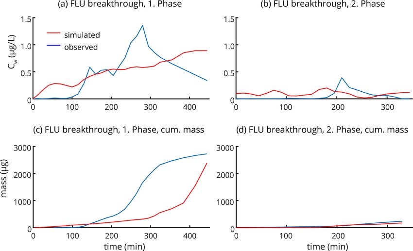
1486                                             A. Sternagel et al.: Simulation of reactive solute transport in the critical zone

and is hence added as upward velocity, contrary to the down-
ward drift term (Roth and Hammel, 1996). The third term
of Eq. (5) describes diffusive displacement of water parti-
cles determined by the soil moisture gradient and controlled
by diffusivity D(θ ) (m s−1 ) in combination with the random
walk concept. Here, the expression (θr + i · 1θ ) represents
the aforementioned fraction of the actual soil water content
θ(t) (cf. Sect. 2.1) that is stored in a certain pore size of the
soil domain. Note that i is the number of a bin of NB total
bins representing the certain pore size in which the particle
is stored, θr the residual soil moisture, 1θ the size/water con-
tent range of a bin, and Z a random number from a standard
normal distribution.                                                  Figure 1. Particle binning concept. All particles within an element
                                                                      of the Euler grid are distributed to bins (i.e. red rectangles) repre-
Model assumptions                                                     senting fractions of the actual soil water content stored in different
                                                                      pore sizes. Displacements of these particle fractions are determined
The above-described distribution of water particle displace-          by the corresponding flow velocities and diffusivities (figure taken
ments to different pore sizes/bins (“binning”) was the key            from Sternagel et al., 2019).
to simulating soil water dynamics in the case of pure matrix
flow, in agreement with the Richards equation and field ob-
servations (Zehe and Jackisch, 2016). This binning of parti-          Solute transport
cle displacements is defined by the water diffusivity and hy-
draulic conductivity curve. These curves are separated into           Each water particle is characterized by its position in the soil
NB bins, using a step size of 1θ = (θ (t)−θ NB
                                                r)
                                                   from the resid-    domain, water mass, and a solute concentration. This means
ual moisture θr to the actual moisture θ (t) (Fig. 1). Zehe and       that there is no second species of particles representing so-
Jackisch (2016) found that 800 bins are sufficient to resolve         lutes. Each water particle is tagged by a solute mass that
both curves. This particle binning concept enables also the           is defined by the product of solute concentration and wa-
simulation of non-equilibrium conditions in the water infil-          ter particle volume. Hence, we do not use a separate, spe-
tration process. To that end, a second type of particles (event       cific equation for the transport of solutes in LAST. Solutes
particles) is introduced to treat infiltrating event water. These     are displaced together with the water particles according to
particles initially travel, purely by gravity, in the largest pores   the varying particle displacements defined by Eq. (5). Sub-
and experience a slow mixing with pre-event particles in the          sequent to the displacement, diffusive mixing and redistribu-
soil matrix during a characteristic mixing time. This non-            tion of solutes among all water particles in an element of the
equilibrium flow in the matrix is laminar, as Eq. (5) is based        Euler grid is calculated by summing their solute masses and
on the theory of the Richards equation (Eq. 1). An adaptive           dividing this total mass amount by the number of water par-
time stepping is used to fulfil the Courant criterion to ensure       ticles present. Due to this perfect solute mixing process, the
that particles do not travel farther than the length of a grid        solute mass carried by a water particle may vary in space and
element dz in a time step.                                            time. In this context, it is important to recall that the use of
                                                                      an Euler grid to calculate soil water contents and solute con-
2.2.2   Transport of conservative solutes and the
                                                                      centrations in Lagrangian models may lead to the problem of
        macropore domain
                                                                      artificial over-mixing (e.g. Boso et al., 2013; Cui et al., 2014;
In our previous work (Sternagel et al., 2019), we extended the        e.g. Berkowitz et al., 2016). This is because water and solutes
scope of the Lagrangian approach (i) to account for simula-           are assumed to mix perfectly within the elements of the Euler
tions of water and solute transport in soils as well as (ii) by a     grid, which may lead to a smoothing of gradients in the case
structural macropore/preferential flow domain and included            of coarse grid sizes. This might lead to overestimates of con-
both extensions in the LAST-Model. We tested this extended            centration dilution while solutes infiltrate into and distribute
approach using bromide tracer and macropore data of plot-             within the soil domain (Green et al., 2002, cf. Sect. 6.2).
scale irrigation experiments at four study sites and compared
it to simulations of HYDRUS 1-D. At two sites dominated by            Macropore domain
well-mixed matrix flow, both models showed equal perfor-
mance, but at two preferential-flow-dominated sites, LAST             LAST offers a structured preferential flow domain consist-
performed better. We refer to Sternagel et al. (2019) for ad-         ing of a certain number of macropores (Fig. 2a). Macropores
ditional details on the model and results.                            are classified into the three depth classes – deep, medium, or
                                                                      shallow – to reflect the corresponding variations of macrop-
                                                                      ore depths observed at a study site. With this approach, we

Hydrol. Earth Syst. Sci., 25, 1483–1508, 2021                                           https://doi.org/10.5194/hess-25-1483-2021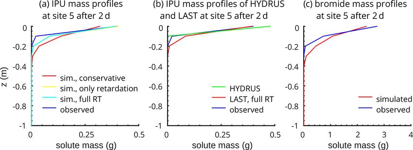
A. Sternagel et al.: Simulation of reactive solute transport in the critical zone 1487
may account for a depth-dependent exchange of water and 3.1 Retardation of solute transport via non-linear
solutes between the matrix and macropore domains. The pa- sorption between water and solid phase
rameterization of the preferential flow domain may hence
largely rely on observable field data, such as the number 3.1.1 Implementation of retardation
of macropores of certain diameters, their length distribution,
and hydraulic properties. When such field observations are The interplay of adsorption and desorption characterizes the
not available, the parameters can be estimated by inverse retardation process and implies that the transport velocity
modelling using tracer data. The actual water content and of a reactive solute is smaller than the fluid velocity. This
the flux densities of the topsoil control infiltration and dis- is commonly represented by reducing the solute transport
tribution of water particles to both domains. The soil water velocity by a retardation factor. This retardation factor de-
content determines the matric potential and hydraulic con- scribes the ratio between the fluid velocity and the solute
ductivity of the soil matrix, while flow in macropores is con- transport velocity based on the slope of a sorption isotherm.
trolled by friction and gravity. After the infiltration, macro- However, this concept is not applicable in our framework be-
pores gradually fill from the bottom to the top by assuming cause solute masses are carried by the water particles and
purely gravity-driven, advective flow in the macropore do- travel hence at the same velocity as water. We thus explicitly
main (Fig. 2b). Interactions among macropores and the ma- represent sorption processes by a related, explicit transfer of
trix are represented by diffusive mixing and exchange of wa- solute masses between the water and soil solid phase. The
ter and solutes between both flow domains, which depends mass exchange rates are variable in time, as the solute con-
also on the matric potential and water content (Fig. 2c). centrations in the water and solid phase also vary between
We provide a detailed description of Fig. 2 with the struc- time steps. In each time step, the solute mass exchange be-
ture of the macropore domain and the infiltration and fill- tween both phases is calculated by using the non-linear Fre-
ing of macropores, as well as exchange processes between undlich isotherms of the respective solute and rate equations
macropores and the matrix, in the Appendix. (Eq. 6 for adsorption, Eq. 7 for desorption).
m
beta p
mrs (t) = mrs (t − 1t) − Kf Crs , (6)
3 Concept and implementation of reactive solute ρ
transport into the LAST-Model where mhrs (kg)
i 1
is the reactive solute mass of a parti-
kg beta
The main objective of this study is to present a method to cle, Kf kg the Freundlich coefficient/constant, Crs
simulate fluid flow with reactive solute transport in struc-
tured, partially saturated soils, using a Lagrangian perspec- (kg m−3 ) the reactive solute concentration of a particle, beta
tive. The method is illustrated through the implementation of (–) the Freundlich exponent, mp (kg) the water mass of a par-
a routine into the LAST-Model, to simulate the movement ticle, ρ (kg m−3 ) the water density, t (s) the current simula-
of reactive substances through the soil zone under the influ- tion time, and 1t (s) the time step. Note that Kf and beta are
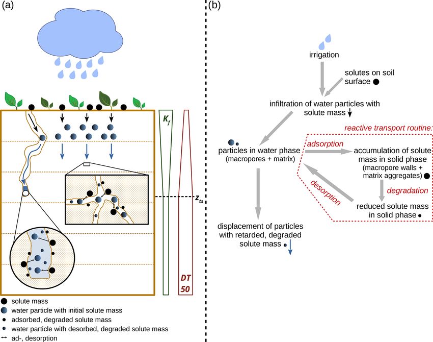
ence of sorption and degradation processes (Fig. 3). This is both empirical constants that determine the shape and slope
achieved by assigning an additional reactive solute concen- of the sorption isotherm of a respective substance. Both are
tration Crs (kg m−3 ) to each water particle. A water parti- often described as dimensionless coefficients, but Kf can ac-
cle can hence carry a reactive solute mass mrs (kg), which tually adopt different forms to balance the units of the equa-
is equal to the product of reactive solute concentration and tion, particularly when beta is not equal to 1.
its water volume. Transport and mixing of the reactive so- The reversed desorption of adsorbed solutes from the soil
lute masses within a time step are simulated in the same way solid phase to the water particles, in the case of a reversed
as for the conservative solute (cf. Sect. 2.2.2) (Sternagel et solute concentration gradient between water and solid phase,
al., 2019). After the solute mixing and mass redistribution is equally calculated (Eq. 7). It uses the solute concentration
among water particles, the reactive solute mass of each par- in the sorbing solid phase Crs_solid (kg m−3 ), which requires
ticle can change due to a non-linear mass transfer (adsorp- the adsorbed solute mass and the volume of the phase Vsoil
tion, desorption) between water particles and the sorption (m3 ). In this way, the total desorbed solute mass is calcu-
sites of the adsorbing solid phase, which are determined by lated for an entire grid element and must be divided by the
the substance-specific and site-specific Freundlich isotherms present particle number NP (–) to equally distribute the des-
(cf. Sect. 3.1). The adsorbed reactive solute mass in the soil orbed solute mass among the water particles. The sorption
solid phase can then be reduced by degradation following process is hence controlled by a local concentration gradient
first-order kinetics driven by the half-life of the substance between water and the solid phase within an element of the
(cf. Sect. 3.2). These two reactive solute processes take place Euler grid.
in the soil matrix as well as in the wetted parts of the macro-
beta
Kf Crs_solid Vsoil
pores, and their intensity can vary with soil depth as detailed
in the following sections. mrs (t) = mrs (t − 1t) + (7)
NP
https://doi.org/10.5194/hess-25-1483-2021 Hydrol. Earth Syst. Sci., 25, 1483–1508, 2021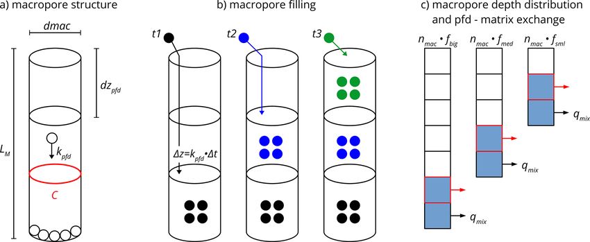
1488                                              A. Sternagel et al.: Simulation of reactive solute transport in the critical zone

Figure 2. Conceptual visualization of (a) the structure of a single macropore, (b) the macropore filling with gradual saturation of grid
elements, exemplarily shown for three points in time (t1 − t3 ), whereby at each time new particles (differently coloured related to the current
time) infiltrate the macropore and travel into the deepest unsaturated grid element, and (c) the macropore depth distribution and diffusive
mixing of water from saturated parts of macropores (blue filled squares) into the matrix (cf. Sect. 2.2.2). The figure was adapted from
Sternagel et al. (2019).

Figure 3. (a) Overview sketch of sorption and degradation processes in the soil domain. Down to the predefined depth zts (m), we assume
the topsoil with linearly decreasing Kf and linearly increasing DT50 values to account for the depth dependence of sorption and degradation,
respectively. Below zts in the subsoil, we assume constant values. (b) Flow chart to illustrate the sequence of reactive solute transport. The
pictograms of the sketch are assigned to the respective positions and steps of the flow chart.

Hydrol. Earth Syst. Sci., 25, 1483–1508, 2021                                                https://doi.org/10.5194/hess-25-1483-2021
A. Sternagel et al.: Simulation of reactive solute transport in the critical zone                                              1489

3.1.2   Assumptions for the parameterization of the                  nificant degree once water is stagnant in the saturated parts
        sorption process                                             of the macropores (Bolduan and Zehe, 2006). This stagnancy
                                                                     facilitates the possibility for sorption of reactive solutes be-
Generally, sorption is a non-linear process, which reflects the      tween macropore water and the macropore walls. The macro-
limited availability of adsorption sites and, hence, exchange        pore sorption processes are also described and quantified by
rate limitations. This may cause imperfect sorption, which           the Freundlich approach and Eq. (6).
can lead to the observation of early mass arrivals and long
tailings in breakthrough curves (e.g. Leistra, 1977). Thus, our      3.2     First-order degradation of adsorbed solutes in soil
approach calculates the non-linear adsorption or desorption                  solid phase
of solute masses, as a function of the solute concentration
or loading of the sorption surfaces of the sorbent. Hence, in        3.2.1    Implementation of degradation
a given time step, the higher the solute concentration in the
                                                                     Reactive solutes such as pesticides are commonly biode-
solid phase, the fewer the solute masses that can be addi-
                                                                     graded and therewith transformed into metabolite/child com-
tionally adsorbed from the water phase, and vice versa. In
                                                                     pounds by the metabolism or co-metabolism of microbial
the approach developed here, the sorption process proceeds
                                                                     communities that are present mainly on the surfaces of soil
only until a concentration equilibrium between both phases
                                                                     particles. The immobilization of a reactive substance, due to
is reached. At this point, there is no further adsorption or des-
                                                                     adsorption, favours degradation when the residence time in
orption of solute masses until the concentration of one phase
                                                                     the adsorbing solid phase is sufficiently long for metaboliza-
is again disequilibrated by, for example, the infiltration of
                                                                     tion. Many pesticides are subject to co-metabolic degrada-
water into the water phase or by solute degradation in the
                                                                     tion, which often follows first-order kinetics and can hence
solid phase. In the case that the concentration of a reactive
                                                                     be characterized by an exponential decay function
solute in the water phase is higher than its solubility, the ex-
cess solute masses leave the solution and are adsorbed to the        Ct = C0 e−k t ,                                             (8)
soil solid phase.
   With regard to pesticides, the major pesticide sorbent is         where Ct (kg m−3 ) is the concentration of the pesticide after
soil organic matter, and its quantity and quality determine to       the time t (s), C0 (kg m−3 ) the initial concentration, and k
a large fraction the soil sorption properties (Farenhorst, 2006;     (s−1 ) the degradation rate constant.
Sarkar et al., 2020). Several studies revealed that in the top-         Based on the first-order kinetics of Eq. (8), we apply a
soil, enhanced sorption of pesticides occurs due to the often        mass rate equation (Eq. 9) for the degradation of adsorbed
high content of organic matter, which may reflect bioavail-          solute masses on the macroscopic scale of an element of the
ability by an increased number of sorption sites in the non-         Euler grid:
mineralized organic matter (e.g. Clay and Koskinen, 2003;
Jensen et al., 2004; Boivin et al., 2005; Rodríguez-Cruz et                                                1t
                                                                     msp (t + 1t) = msp (t) 1 − kd                ,             (9)
al., 2006). This implies that the conditions in the topsoil gen-                                        86 400
erally facilitate the sorption of dissolved solutes. While dif-
ferent depth profiles of the Kf value could be implemented           where msp (t) and msp (t + 1t) (kg) are the reactive solute
depending on available data, to account for this depth depen-        masses in the soil solid phase of the current time step and of
dence of sorption processes, here we apply a linearly decreas-       the next time step after degradation and 1t (s) the time step.
ing distribution of the Kf value over the grid elements of the       The kinetics of this degradation process are determined by
soil domain between two predefined upper and lower value             the half-life DT50 (d) of the respective substance, with the
limits for the topsoil. The depth of the topsoil (zts ) can be ad-   relationship between DT50 and a daily degradation kd (d−1 )
justed individually and for our applications; here, we set it to     given by
50 cm. Below this soil depth, we assume the subsoil and ap-
                                                                             ln (2)
ply constant Kf values. The exact Kf parameterizations of the        kd =           .                                           (10)
respective model setups at the different sites are explained in              DT50
Sect. 4.2.1 and 4.2.2 and summarized in Table 2.                     3.2.2    Assumptions for the parameterization of the
                                                                              degradation process
Sorption in macropores
                                                                     Turnover and degradation of pesticides depend in general on
While sorption generally controls pesticide leaching in the          the substance-specific chemical properties and the microbial
soil matrix, the processes are different in macropores. Sorp-        activity in soils (Holden and Fierer, 2005). Microbial activ-
tion in macropores is often limited because the timescale of         ity in soil depends on many factors, including organic matter
vertical advection is usually much smaller than the time re-         content, pH, water content, temperature, redox potential, and
quired by solute molecules to diffuse to the macropore walls         carbon / nitrogen ratio. As these factors are usually highly
(Klaus et al., 2014). However, sorption may occur to a sig-          heterogeneous in space, considerable research has focused

https://doi.org/10.5194/hess-25-1483-2021                                           Hydrol. Earth Syst. Sci., 25, 1483–1508, 2021
1490 A. Sternagel et al.: Simulation of reactive solute transport in the critical zone
on spatial differences in pesticide turnover potentials. Some timescales of 7 and 21 d. Finally, we evaluate the method by
of these studies determined that pesticide turnover rates typ- simulating the breakthrough and remobilization of the herbi-
ically decrease within the top metre of the soil matrix (e.g. cide flufenacet that was observed in the tile drain of a field
El-Sebai et al., 2005; Bolduan and Zehe, 2006; Eilers et al., site within two irrigation phases: 1 d and 3 weeks after sub-
2012). This is because the topsoil provides conditions that fa- stance application.
cilitate enhanced microbial activity (Fomsgaard, 1995; Bend-
ing et al., 2001; Bending and Rodriguez-Cruz, 2007). The 4.1 Characterization of the irrigation experiments
simplest way to account for such a depth-dependent degra-
dation is a linear increase of the DT50 value from the topsoil 4.1.1 Study area: the Weiherbach catchment
surface to a predefined depth zts , which is set to 50 cm. This
The Weiherbach valley extends over a total area of 6.3 km2
value is in line with the assumption of the depth-dependent
and is located in the southwest of Germany. The land is used
Kf parameter and was estimated based on the findings of the
mainly for agriculture. The basic geological formation of the
aforementioned studies. In the subsoil below 50 cm, we ap-
valley is characterized by a Pleistocene loess layer up to 15 m
ply constant DT50 values (cf. Sect. 3.1). The exact DT50 pa-
thick, which covers Triassic Muschelkalk marl and Keuper
rameterizations of the respective model setups at the different
sandstone. At the foot of hills, the hillslopes show a typical
sites are explained in Sect. 4.2.1 and 4.2.2 and summarized
loess catena with erosion-derived Colluvic Regosols, while
in Table 2.
at the top and in the middle parts of hills, mainly Calcaric
Degradation in macropores Regosols or Luvisols are present. More detailed informa-
tion on the Weiherbach catchment is provided in Plate and
The presence of macropores allows pesticides to bypass the Zehe (2008).
topsoil matrix, while they may infiltrate and thus be more
4.1.2 Pesticides isoproturon (IPU) and flufenacet (FLU)
persistent in the deeper subsoil matrix where the turnover
potential is decreased. As biopores like worm burrows often IPU is an herbicide which is commonly applied in crops to
constitute the major part of macropores in agricultural soils, a control annual grasses and weeds. IPU has a moderate water
number of studies have focused on their key role in pesticide solubility of 70.2 mg L−1 and is regarded as non-persistent
transformation (e.g. Binet et al., 2006; Liu et al., 2011; Tang (mean DT50 in field: 23 d) and moderately mobile (mean
et al., 2012). These studies consistently revealed an elevated Kf = 2.83) in soils (see also typical Kf and DT50 value
bacterial abundance and activity in the immediate vicinity of ranges in Table 2). IPU is ranked as carcinogenic, and its
worm burrows (Bundt et al., 2001; Bolduan and Zehe, 2006), turnover in soils forms, mainly, the metabolite desmethyliso-
comparable to the optimum conditions in topsoil. This is at- proturon (Lewis et al., 2016).
tributed to a positive effect of enhanced organic carbon, nutri- FLU is an herbicide that can be applied for a broad spec-
ent, and oxygen supply that may lead to increased adsorption trum of purposes but is used especially in combination with
and degradation rates in macropores. Thus, we assume that other herbicides to control grasses and broad-leaved weeds.
degradation also takes place in the adsorbing phase of the FLU is regarded as moderately soluble (51 mg L−1 ) and is
macropores, which can be quantified with Eq. (9). We apply not highly volatile (mean Kf = 4.38) but may be quite per-
different Kf and DT50 values in the macropores that are in sistent in soils (up to DT50 in field: 68 d) under certain con-
the range of the topsoil values (cf. Table 2). ditions. FLU is classified as moderately toxic to humans,
and its turnover in soils mainly forms the metabolites FOE
sulfonic acid, FOE oxalate, and FOE alcohol (Lewis et al.,
4 Model application tests 2016).
The proposed method to simulate reactive solute transport 4.1.3 Plot-scale experiments of Zehe and Flühler (2001)
in a Lagrangian approach is tested by using LAST to simu- at the well-mixed site (site 5) and the
late irrigation experiments with conservative bromide tracer preferential-flow-dominated site (site 10)
and the herbicide IPU as a representative reactive substance,
at two study sites in the Weiherbach catchment (Zehe and At site 5, the soil moisture and soil properties were initially
Flühler, 2001). Here, conservative means that a solute is nei- measured on a defined plot area of 1.4 m × 1.4 m. Before the
ther subject to sorption nor to degradation. These two sites irrigation, 0.5 g of IPU was applied, distributed evenly, on
are dominated by either matrix flow under well-mixed con- the surface of the plot area. After 1 d, the IPU loaded plot
ditions (site 5) or preferential macropore flow (site 10) on a area was irrigated by a rainfall event of 10 mm h−1 of wa-
timescale of 2 d. These experiments are also simulated with ter for 130 min with 0.165 g L−1 of bromide. After another
the HYDRUS 1-D model. To test the method on simulation day, soil samples were taken along a vertical soil profile of
periods longer than 2 d, we use data from an additional plot- 1 m × 1 m in a grid of 0.1 m × 0.1 m. Thus, 10 soil samples
scale (site P4) irrigation experiment (Klaus et al., 2014) on were collected in each 10 cm depth interval down to a to-
Hydrol. Earth Syst. Sci., 25, 1483–1508, 2021 https://doi.org/10.5194/hess-25-1483-2021A. Sternagel et al.: Simulation of reactive solute transport in the critical zone 1491
tal depth of 1 m. In subsequent lab analyses, the IPU and trations were measured at the outlet of a tile-drain tube. The
bromide concentrations of all samples were measured. The tube drained the entire field site and was located 1–1.2 m be-
soil at site 5 is a Calcaric Regosol (IUSS Working Group low the surface. Before irrigation, a total of 40 g FLU was
WRB, 2014), and flow patterns reveal a dominance of well- applied on the surface of the 400 m2 field site. In a first ir-
mixed matrix flow without considerable influence of macro- rigation phase, the field site was irrigated in three individual
pore flows. This is the reason for using site 5 to evaluate blocks with a total precipitation of 41 mm over 215 min, and
our reactive solute transport approach under well-mixed flow simultaneously, water samples were taken at the outlet of the
conditions. Table 1 provides all experimental data. tile-drain tube. These samples were analysed for FLU as ex-
The experiment at site 10 was conducted similarly with plained in Klaus et al. (2014). After a period of 3 weeks, in
the initial application of 1.0 g of IPU on the soil plot and 1 d which the field site remained untouched without further ir-
later a block rainfall of 11 mm h−1 for 138 min. The soil at rigation and FLU application, the field site was then again
site 10 can be classified as Colluvic Regosol (IUSS Working irrigated in two individual blocks with a total precipitation of
Group WRB, 2014) and shows numerous worm burrows that 40 mm over 180 min and the FLU concentration in the tile-
can facilitate preferential flow. Hence, we select study site 10 drain outflow measured. The objective was to examine the
for the evaluation of our reactive solute transport approach breakthrough of remobilized FLU that was previously ad-
during preferential flow conditions. The density and depth sorbed in soil.
of the worm burrow systems were examined extensively at The soil of the field site is again a Colluvisol (IUSS
this study site. Horizontal layers in different depths of the Working Group WRB, 2014). Overall, the soil exhibits two
vertical soil profile were excavated (cf. Zehe and Blöschl, ploughed layers between 0–10 and 10–35 cm above a third,
2004; van Schaik et al., 2014), and in each layer the number unaffected Colluvisol layer (Klaus and Zehe, 2010). Klaus
of macropores was counted, and their diameters and depths and Zehe (2010) also found that 10 macropores/m2 reaching
were measured. These detailed measurements provided an into the depths of the tile-drain tube is a good estimate for
extensive dataset of the macropore network. Table 1 again simulations at this study site. Initial soil water contents and
contains all experimental data. all further experimental parameters are listed in Table 4.
4.1.4 Plot- and field-scale experiments of Klaus et 4.2 Model setups
al. (2014)
To compare our 1-D simulation results to the observed 2-D
Klaus et al. (2014) conducted irrigation experiments in the concentration data of the plot-scale experiments, the latter
Weiherbach catchment to corroborate the importance of are averaged laterally in each of the 10 cm depth intervals.
macropore connectivity to tile drains for tracer and pesti- Note that the corresponding observations provide solute con-
cide leaching into surface waters. A series of three irriga- centration per dry mass of the soil, while the LAST-Model
tion experiments with bromide tracer, IPU, and FLU were simulates concentrations in the water phase and adsorbed so-
performed on a 20 × 20 m field site, which also included the lute masses in the soil solid phase, respectively. We thus com-
sampling of these substances in different plot-scale soil pro- pare simulated and observed solute masses and not concen-
files. We focus first on the plot-scale experiment in which the trations in the respective depths. Note that the experimental
field site was irrigated in three individual blocks with a to- parameters in Tables 1, 3, and 4 are measured data from the
tal precipitation sum of 34 mm over 220 min. Additionally, a above-described experiments and can be used directly to pa-
total of 1600 g of bromide was applied on the field site. We rameterize the LAST-Model without fitting. In Sternagel et
concentrate on site P4 where soil samples were collected in a al. (2019), we explain in detail how the observed data are
0.1 m × 0.1 m grid down to a depth of 1 m after 7 d and their processed, particularly for the macropore domain, and ex-
corresponding bromide concentrations measured. Patterns of plain the model sensitivity to the uncertainty range of ob-
worm burrows in the first 15 cm of the soil were also exam- served data (e.g. to the saturated hydraulic conductivity).
ined (Table 3). The present soil is a Colluvisol (IUSS Work-
ing Group WRB, 2014), with a strong gleyic horizon present 4.2.1 Model setups of simulations at the well-mixed
in a depth between 0.4 and 0.7 m, which causes a decreasing plot site (site 5)
soil hydraulic conductivity gradient with depth that leads to
almost stagnant flow conditions in the subsoil (Klaus et al., LAST-Model setup at the well-mixed site (site 5)
2013). In general, the experiment design, soil sampling, and
data collection are similar to the experiments of Zehe and As site 5 is dominated by well-mixed matrix flow, we deac-
Flühler (2001). Initial soil water contents and all further ex- tivate the macropore domain of LAST and simulate IPU and
periment parameters as well as the soil properties at the field bromide transport solely in the matrix domain at this site.
site are listed in Table 3. Without the influence of macropores, we assume here only
Second, we focus on two other irrigation experiments of small penetration depths of solutes through the first top cen-
Klaus et al. (2014) on the field scale in which FLU concen- timetres of the soil, in line with previous simulations at other
https://doi.org/10.5194/hess-25-1483-2021 Hydrol. Earth Syst. Sci., 25, 1483–1508, 20211492 A. Sternagel et al.: Simulation of reactive solute transport in the critical zone
well-mixed sites in the Weiherbach catchment (Sternagel et reactive transport routine to account for the remarkably vari-
al., 2019). This means that solutes may remain in the upper able value ranges of Kf and DT50 reported in various studies
part of the topsoil, so that a depth-dependent parameteriza- (e.g. Bolduan and Zehe, 2006; Rodríguez-Cruz et al., 2006;
tion of sorption and degradation (cf. Sect. 3.1, 3.2) appears, Bending and Rodriguez-Cruz, 2007; Lewis et al., 2016). To
as a first guess, not necessary at this site. Thus, we apply account for the related uncertainty range of the reactive trans-
constant values of Kf and DT50 (Table 2) and use mean val- port behaviour of IPU, we distinguish between two parame-
ues under field conditions for IPU from the Pesticide Prop- ter configurations for a rather weak reactive transport of IPU
erties Database (PPDB) (Lewis et al., 2016). Consistent with and a strong reactive transport with enhanced retardation and
the experiments, we use a matrix discretization of 0.1 m. Ini- degradation of IPU (Table 2). To evaluate solely the impact
tially, the soil domain contains 2 million water particles but of the Kf value on the model sensitivity, we furthermore per-
no solute masses. All further experiment and simulation pa- form a simulation at site 10 only with activated sorption and
rameters are shown in Table 1. deactivated degradation. Table 1 provides all relevant simu-
lation and experiment parameters.
HYDRUS 1-D setup at the well-mixed site (site 5)
HYDRUS 1-D setup at the preferential-flow-dominated
The simulation with HYDRUS 1-D at the well-mixed site site (site 10)
(site 5) is conducted with a single porosity model (van
Genuchten–Mualem) and an equilibrium model for water
The simulations with HYDRUS 1-D at the preferential-
flow and solute transport, respectively, with the Freundlich
flow-dominated site (site 10) are performed with the same
approach for sorption and first-order degradation. At the up-
model setups, soil properties, and initial and boundary con-
per domain boundary, we select atmospheric conditions with
ditions, as well as reactive transport parameters, as for the
a surface layer and variable infiltration intensities. At the
simulations with LAST (cf. Tables 1, 2). In contrast, we
lower boundary, we assume free drainage conditions. In gen-
select a dual-permeability approach for water flow (Gerke
eral, we use the same soil hydraulic properties, model se-
and van Genuchten, 1993) and solute transport (physical
tups, initial conditions, and reactive transport parameters as
nonequilibrium) at this site. These approaches distinguish
for LAST (cf. Tables 1, 2).
between matrix and fracture domains for water flow and so-
lute transport. It applies the Richards equation for water flow
4.2.2 Model setups of simulations at the
in each domain, with domain-specific hydraulic properties.
preferential-flow-dominated plot site (site 10)
The advection–dispersion equation is used to simulate solute
transport and mass transfer between both domains, including
LAST-Model setup for simulations at the
terms for reactive transport with retardation and degradation
preferential-flow-dominated site (site 10)
(Gerke and van Genuchten, 1993). While we apply the same
soil hydraulic properties in the matrix (cf. Table 1) as for the
We use an available, extensive macropore dataset to parame-
LAST simulations, the macropore domain in HYDRUS gets
terize the macropore domain at site 10. Table 1 provides the
a faster character with a Ks value of 10−3 m s−1 . We also se-
depth distribution of the macropore network, mean macrop-
lect the Freundlich approach for sorption processes and first-
ore diameters, and the distribution factors. The study of Ster-
order degradation.
nagel et al. (2019) explains in detail how the macropore do-
main of LAST is parameterized based on available field mea-
surements. We vertically discretize the macropores in steps 4.2.3 LAST-Model setup of 7 and 21 d simulations at
of 0.05 m and assume that they initially contain neither water the plot site (site P4)
particles nor solute masses. A maximum of 10 000 possible
particles that can be stored in a single macropore, and hence We perform simulations for conservative bromide tracer and
the total possible number of particles in the entire macrop- reactive IPU at site P4 for periods of 7 and 21 d using the
ore domain, is given by multiplication with the total num- parameters in Table 3, respectively. Based on examination
ber of macropores. The studies of Ackermann (1998) and of the macropore network, we again derive the parameteri-
Zehe (1999) provide further descriptions of site 10 and the zation of the macropore domain (Table 3). In line with the
macropore network. LAST-Model setups in Sect. 4.2.1 and 4.2.2, we apply the
As the heterogeneous macropore network allows for a same discretization of the matrix dz (0.1 m) and macropore
rapid bypassing of solutes, we expect a considerable pen- (0.05 m) domain as well as number of particles in both do-
etration into different soil depths. We use depth-dependent mains (2 million; 10 k per macropore grid element). Addi-
values of Kf and DT50 for IPU in the matrix and in the tionally, we perform another 7 d simulation for bromide with
macropores to account for a depth-dependent retardation and a finer matrix discretization dz of 0.05 m. Initially, macrop-
degradation (Table 2) for the simulations at site 10. Further- ores and matrix contain no solute masses, and the macropores
more, we here use different parameterization setups of the also contain no water.
Hydrol. Earth Syst. Sci., 25, 1483–1508, 2021 https://doi.org/10.5194/hess-25-1483-2021A. Sternagel et al.: Simulation of reactive solute transport in the critical zone 1493
For the simulation of reactive IPU transport, we again ap- case of the simulation with retardation and no degradation
ply the weak and strong reactive transport parameterizations (yellow profile), the simulated mass profile matches the ob-
with the depth-dependent Kf and DT50 values of the simu- served profile in the first 10 cm because retardation causes
lations at site 10 (cf. Table 2). Additionally, we apply here a mass accumulation. With additional degradation (light blue
mean reactive transport parameterization. An evaluation with profile), the solute masses in the first 10 cm are then slightly
observed IPU mass profiles is not possible here because ro- reduced. The influence of degradation is relatively small, due
bust experimental data are missing. All relevant parameters to the moderate DT50 value of 23 d and the short simulation
of the 7 and 21 d simulations at P4 are listed in Table 3. period of 2 d, but it is nevertheless detectable. Overall, we
find that there are indeed noticeable differences (RMSE dif-
4.2.4 LAST-Model setup of the FLU breakthrough ference of 7.3 %) between the IPU profiles of the conserva-
simulations at the field site tive, reference simulation and the reactive transport simula-
tion with retardation and degradation, which is also in better
We perform a simulation of FLU concentrations, which mi- accord with the observed mass profile, reflected by a smaller
grate from the soil surface into the depth of the tile-drain tube RMSE value of 0.027 g (5.5 % of applied mass). At the end
(1 m), over the entire field site, in each of the two irrigation of the simulated period of 2 d, a total IPU mass of 0.014 g
phases. After the first irrigation phase, we assume steady- is degraded, while the observed profile has a mass deficit of
state flow conditions, as Klaus et al. (2014) found that the 0.078 g corresponding to a recovery rate of 84 %. This ob-
flow in the tile-drain tube already approached its initial value served mass deficit cannot be explained exclusively by degra-
after roughly 500 min. This implies hydraulic equilibrium be- dation. It might be the result of additional mass losses in the
tween gravity and capillary forces and thus zero soil water experiment execution and lab analyses.
flow in the period of 3 weeks between the first and second
irrigation phase. Nevertheless, adsorption and degradation of 5.1.2 IPU transport simulated with HYDRUS 1-D
FLU are still active and simulated using mean Kf and DT50
values in soil (Lewis et al., 2016, cf. Table 4) during the 3 The IPU mass profile simulated with HYDRUS 1-D
weeks until the second irrigation phase starts. (Fig. 4b), with activated reactive transport, shows similar
The parameterization of the macropore domain with the mass patterns compared to LAST and the observed profile
number and depth of macropores per square metre follows with a RMSE value of 0.036 g (7.3 % of applied mass). While
the recommendations of Klaus and Zehe (2010). In line with HYDRUS overestimates the IPU masses at the soil surface,
the previous LAST-Model setups, we apply the same dis- considering a stronger retardation compared to the observa-
cretization of the matrix dz (0.1 m) and macropore (0.05 m) tion and the LAST results, it simulates the observed masses
domain as well as the number of particles in both domains in 10–20 cm soil depth quite well. In these depths, LAST
(2 million; 10 k per macropore grid element). Macropores overestimates masses with a maximum penetration depth of
and matrix again contain no solute masses, and the macro- 30 cm, which is 10 cm deeper than observed. Overall, the re-
pores also contain no water, initially. All further simulation sults of HYDRUS and LAST are in comparable agreement
parameters of the FLU breakthrough simulations are listed in with the observed profile. HYDRUS simulates a total, de-
Table 4. graded IPU mass of 0.017 g, which is in the range of the
LAST results (cf. Sect. 5.1.1). This means that in both mod-
els, the total degradation is similar, but the distribution of the
5 Results remaining IPU masses over the soil profile differs.
In the following sections, we present simulated vertical mass 5.1.3 Bromide transport simulated with LAST
profiles of bromide and IPU at the different plot-scale study
sites (sites 5, 10, and P4), as well as breakthrough time series Bromide slightly percolates into greater depths during the
of FLU concentrations at the field site (cf. Sect. 4.1). short-term irrigation experiment (Fig. 4c) compared to the
retarded and degraded IPU (cf. Fig. 4a). The results gener-
5.1 Simulation results at the well-mixed plot site (site ally underline that the Lagrangian approach is able to sim-
5) after 2 d ulate conservative solute transport under well-mixed condi-
tions, as we have already shown in our previous study (Ster-
5.1.1 IPU transport simulated with LAST nagel et al., 2019). The results further show that the approach
is capable of treating both conservative tracers and reactive
In Fig. 4a, the reference simulation treating IPU as conserva- substances.
tive (red profile) overestimates the transport of IPU into soil
depths lower than 10 cm, with a maximum penetration depth
of 40 cm. This leads in turn to simultaneous underestimation
of masses in shallow depths near the soil surface (root mean
square error, RMSE: 0.064 g, 12.8 % of applied mass). In the
https://doi.org/10.5194/hess-25-1483-2021 Hydrol. Earth Syst. Sci., 25, 1483–1508, 20211494 A. Sternagel et al.: Simulation of reactive solute transport in the critical zone
Table 1. Parameters of IPU plot-scale experiments and simulations, as well as soil hydraulic parameters according to van Genuchten (1980)
and Mualem (1976), at sites 5 and 10, where Ks is the saturated hydraulic conductivity, θs the saturated soil water content, θr the residual
soil water content, α the inverse of an air entry value, n a quantity characterizing pore size distribution, s the storage coefficient, and ρb the
bulk density. Further, mac. big, mac. med, and mac. sml describe the lengths of big, medium, and small macropores as well as fbig , fmed ,
and fsml are the respective distribution factors to split the total number of macropores into these three macropore depths (cf. Sect. 2.2.2). For
further details on these parameters, see Sternagel et al. (2019).
Parameter Site 5 Site 10
Experimental parameters
Irrigation duration (hh:mm) 02:10 02:18
Irrigation intensity (mm h−1 ) 10.70 11.00
Applied IPU mass (kg) 5 × 10⁻⁴ 1 × 10⁻³
Recovery rate (%) 84.4 91
Initial soil moisture in 15 cm (%) 23.7 27.8
Soil type Calcaric Regosol Colluvic Regosol
Ks (m s−1 ) 1.00 × 10⁻⁶ 1.00 × 10⁻⁶
θs (m3 m−3 ) 0.46 0.46
θr (m3 m−3 ) 0.04 0.04
α (m−1 ) 4.0 3.0
n (–) 1.26 1.25
s (–) 0.38 0.38
ρb (kg m−3 ) 1300 1500
Number of macropores/m2 (–) – 92
Mean macropore diameter (m) – 0.005
mac. big (m) – 0.8
mac. med (m) – 0.5
mac. sml (m) – 0.2
fbig (–) – 0.14
fmed (–) – 0.37
fsml (–) – 0.49
Simulation parameters
Simulation time t (s) 172 800 (i.e. 2 d)
Time step 1t (s) dynamic
Particle number in matrix (–) 2 million
Water mass of particle in matrix (kg) 1.9 × 10⁻⁴ 2.2 × 10⁻⁴
Particle number in macropore domain (–) – 920 k
Water mass of particle in macropore domain (kg) – 1.6 × 10⁻⁶
5.2 Simulation results at the and degradation, comparing parameterizations for weak and
preferential-flow-dominated plot site (site 10) after strong reactive transport. The shaded area between these pro-
2d files represents the corresponding uncertainty ranges.
In general, the typical “fingerprint” of preferential flow
5.2.1 IPU transport simulated with LAST through macropores is clearly visible in the observed IPU
mass profile. The observed mass accumulations and peaks
fit well to the observed macropore depth distribution (cf. Ta-
Figure 5a and b present results of different simulation se-
ble 1), which implies that water and IPU travelled through the
tups compared to the observed IPU mass profile at site 10
macropores and infiltrated into the matrix in the respective
after 2 d. Both figures comprise the observed profile as well
soil depths where the macropores end. The observed mass
as a profile of a reference simulation treating IPU as con-
profile shows a strong accumulation of IPU masses in depths
servative. Figure 5a focuses on the mass profiles resulting
between 70–90 cm, which cannot be explained by the rela-
from simulations only with activated retardation, using low
tively low number of macropores (∼ 13) in this depth. One
and high Kf values. Figure 5b shows results for simulations
reason for this could be particle-bound transport of IPU at
performed with full reactive transport subject to retardation
Hydrol. Earth Syst. Sci., 25, 1483–1508, 2021 https://doi.org/10.5194/hess-25-1483-2021You can also read