The polarization-encoded self-coherent camera - Astronomy ...
←
→
Page content transcription
If your browser does not render page correctly, please read the page content below
A&A 646, A177 (2021)
https://doi.org/10.1051/0004-6361/202039569                                                                       Astronomy
c ESO 2021                                                                                                         &
                                                                                                                  Astrophysics

                    The polarization-encoded self-coherent camera
                                                                 S. P. Bos

     Leiden Observatory, Leiden University, PO Box 9513, 2300 RA Leiden, The Netherlands
     e-mail: stevenbos@strw.leidenuniv.nl

     Received 1 October 2020 / Accepted 15 December 2020

                                                                 ABSTRACT

     Context. The exploration of circumstellar environments by means of direct imaging to search for Earth-like exoplanets is one of the
     challenges of modern astronomy. One of the current limitations are evolving non-common path aberrations (NCPA) that originate
     from optics downstream of the main wavefront sensor. Measuring these NCPA with the science camera during observations is the
     preferred solution for minimizing the non-common path and maximizing the science duty cycle. The self-coherent camera (SCC) is
     an integrated coronagraph and focal-plane wavefront sensor that generates wavefront information-encoding Fizeau fringes in the focal
     plane by adding a reference hole (RH) in the Lyot stop. However, the RH is located at least 1.5 pupil diameters away from the pupil
     center, which requires the system to have large optic sizes and results in low photon fluxes in the RH.
     Aims. Here, we aim to show that by featuring a polarizer in the RH and adding a polarizing beamsplitter downstream of the Lyot stop,
     the RH can be placed right next to the pupil. This greatly increases the photon flux in the RH and relaxes the requirements on the
     optics size due to a smaller beam footprint. We refer to this new variant of the SCC as the polarization-encoded self-coherent camera
     (PESCC).
     Methods. We study the performance of the PESCC analytically and numerically, and compare it, where relevant, to the SCC. We look
     into the specific noise sources that are relevant for the PESCC and quantify their effect on wavefront sensing and control (WFSC).
     Results. We show analytically that the PESCC relaxes the requirements on the focal-plane sampling and spectral resolution with
     respect to the SCC by a factor of 2 and 3.5, respectively. Furthermore, we find via our numerical simulations that the PESCC has
     effectively access to ∼16 times more photons, which improves the sensitivity of the wavefront sensing by a factor of ∼4. We identify
     the need for the parameters related to the instrumental polarization and differential aberrations between the beams to be tightly
     controlled – otherwise, they limit the instrument’s performance. We also show that without additional measurements, the RH point-
     spread function (PSF) can be calibrated using PESCC images, enabling coherent differential imaging (CDI) as a contrast-enhancing
     post-processing technique for every observation. In idealized simulations (clear aperture, charge two vortex coronagraph, perfect DM,
     no noise sources other than phase and amplitude aberrations) and in circumstances similar to those of space-based systems, we show
     that WFSC combined with CDI can achieve a 1σ raw contrast of ∼3 × 10⁻¹¹ −8 × 10⁻¹¹ between 1 and 18 λ/D.
     Conclusions. The PESCC is a powerful, new focal-plane wavefront sensor that can be relatively easily integrated into existing ground-
     based and future space-based high-contrast imaging instruments.
     Key words. instrumentation: adaptive optics – instrumentation: high angular resolution

1. Introduction                                                          wavefront errors caused by the turbulent Earth’s atmosphere,
                                                                         coronagraphs to suppress starlight, and additional imaging, spec-
The direct imaging of exoplanets is a rapidly growing research           troscopic, and polarimetric post-processing techniques to further
field as it offers exciting opportunities in comparison to indi-         remove the speckle background. The current suite of observing
rect methods such as the transit and radial velocity method. The         and post-processing techniques consists of: angular differential
star and exoplanet light are spatially separated and this there-         imaging (ADI; Marois et al. 2006), reference star differential
fore allows for the direct characterization of the exoplanet and         imaging (RDI; Ruane et al. 2019), spectral differential imaging
(eventually) the search for biomarkers. Furthermore, it can tar-         (SDI; Sparks & Ford 2002), polarimetric differential imaging
get exoplanets at wider separations than practically attainable          (PDI; Kuhn et al. 2001), and coherent differential imaging (CDI;
with indirect methods and does not suffer from diminishing               Guyon 2004). Both ADI and RDI are observing techniques
sensitivity when the exoplanet’s orbit is not edge-on. How-              that are relatively easy to implement, but have been suffering
ever, the direct imaging of exoplanets is not a trivial task and         from temporal stability issues that prevent them to reach high
many technical challenges still have to be solved. For example,          contrasts at small separations. In addition, SDI has been shown
when observing an Earth-like exoplanet around a Solar-type star          to be ineffective at smaller inner working angles, as the radial
at 10 pc, the angular separation is expected to be ∼100 mil-             movement of speckles by spectral diversity is minimal at these
liarcseconds and the contrast ∼1010 in the visible (0.3–1 µm;            separations. However, PDI has achieved impressive results
Traub & Oppenheimer 2010).                                               (van Holstein et al. 2017) and can be simultaneously used for
    Modern ground-based high-contrast imaging (HCI) instru-              exoplanet characterization; still, exoplanets are never 100%
ments (VLT/SPHERE Beuzit et al. 2019; Subaru/SCExAO                      polarized, making this technique not the most efficient discovery
Jovanovic et al. 2015; Gemini/GPI Macintosh et al. 2014;                 method. With CDI, the light in the image is separated into its
Magellan Clay/MagAO-X Males et al. 2018, Close et al. 2018)              coherent and incoherent parts. As the exoplanet’s light is by
deploy extreme adaptive optics (XAO) systems to correct for              definition completely incoherent with the surrounding starlight,

                                                     Article published by EDP Sciences                                       A177, page 1 of 16
A&A 646, A177 (2021)
CDI can use 100% of the exoplanet’s light for the detection. The Fast Atmospheric Self-coherent Camera Technique
This makes it a very promising technique, but it has thus far seen (FAST; Gerard et al. 2018) tackles the second problem by mod-
limited on-sky tests (Bottom et al. 2017). ifying the focal-plane mask of the coronagraph to inject specif-
Typically, the XAO system consists of a deformable mir- ically more light into the RH. This provides the sensitivity to
ror (DM) with a high actuator count and a sensitive wavefront FAST for running at much shorter exposure times and enables
sensor, such as the Shack-Hartmann or Pyramid wavefront it to correct for the rapidly changing residual wavefront errors
sensor, and delivers a high Strehl point-spread-function (PSF) from the XAO system. This technique was tested in simula-
to the instrument. There is a non-common optical path dif- tion with a Lyot coronagraph, and more recently, with a vor-
ference between the science camera and the wavefront sen- tex coronagraph (Gerard & Marois 2020). A lab test validated
sor split-off, in which aberrations occur due to misalignments the coronagraph designs for the FAST concept (Gerard et al.
and manufacturing errors. These so-called non-common path 2019). Another recently developed concept is the fast-modulated
aberrations (NCPA) are not sensed by the main wavefront SCC (FMSCC; Martinez 2019), which aims to address the other
sensor and therefore left uncorrected. Due to changing tem- major disadvantage of the SCC. The FMSCC places the RH
perature, humidity and gravity vector during observations, the right next to the pupil, breaking the original minimum distance
NCPA slowly evolve, making them difficult to calibrate in post- of 1.5 pupil diameters. In order to separate the sidebands from
processing and one of the current limitations in high-contrast the central peak, which are now overlapping, in the OTF, two
imaging (Martinez et al. 2012, 2013; Milli et al. 2016). One images are taken in quick succession with the RH blocked in
solution is to apply a focal-plane wavefront sensor (FPWFS) one of the images. The OTF of this second image only con-
that uses the science images to measure the wavefront aberra- tains the central peak, and when it is subtracted from the first
tions, which can subsequently be corrected by the DM. Ideally, image, the two sidebands are revealed. For the subtraction to
the FPWFS is integrated with the coronagraph to enable simul- successfully reveal the sidebands on ground-based systems with
taneous wavefront measurements and scientific observations. the rapidly changing atmosphere, the system needs to either
A host of different FPWFSs have been developed and tested block the RH at high temporal frequency (∼kHz) to “freeze”
on-sky (Jovanovic et al. 2018), but only a subset has a 100% the atmosphere or to split the post-coronagraphic light into two
science duty cycle (Codona & Kenworthy 2013; Wilby et al. beams: one with and one without RH. The first solution can only
2017; Huby et al. 2017; Guyon et al. 2017; Bos et al. 2019; work for bright targets due to the high switching speeds, and
Miller et al. 2019). the second solution is prone to differential aberrations between
The FPWFS that is most relevant to this work is the self- the two beams. This concept bears great similarities with the
coherent camera (SCC; Baudoz et al. 2005). The SCC places differential OTF WFS (dOTF; Codona 2013), which extracts
a reference hole (RH) in the Lyot stop of a coronagraph in wavefront information by subtracting the OTFs of two PSFs,
an off-axis location. The RH transmits light that is diffracted one of which is formed by an aperture with a small amplitude
by the coronagraph outside of the geometric pupil that would asymmetry.
have otherwise been blocked by the Lyot stop. This light will Here, we present the polarization-encoded self-coherent
propagate to the focal-plane, interfere with the on-axis beam, camera (PESCC), which is a variant of the FMSCC. The PESCC
and generate high-spatial frequency fringes. The focal plane’s features a polarizer in the RH that generates a polarized refer-
electric field is spatially modulated and directly available by ence beam, which, in turn, generates fringes in one polariza-
calculating the Fourier transform (FT) of the image. This oper- tion state, while the orthogonal polarization state is unmodulated
ation results in the optical transfer function (OTF) of the image. by fringes. This is a concept that is very similar to the polar-
The OTF of the SCC consists of three components: the central ization differential OTF wavefront sensor (Brooks et al. 2016).
peak that is the PSF, and two sidebands, which are generated by When the beam is split into two channels by a Wollaston prism
the cross-talk between the fringes and PSF and which contain just before the science camera, it ensures that there are minimal
the electric field estimate. However, for the FT of the image to differential aberrations between the two polarization states. See
properly show the electric field estimate, the RH needs to be at Fig. 1 for an overview of the system architecture. The two polar-
least 1.5 times the pupil diameter from the center of the pupil. ization states can be imaged simultaneously, allowing for longer
This requires the system hosting the SCC to have large-diameter integration times and, therefore, fainter stars can be used as tar-
optics to contain both the reference and the central beam, and gets. For the images of the two polarization states, the OTF can
for the detector to have a high pixel density to properly sam- then be calculated and subtracted to reveal the aberrated electric
ple the fringes in the focal plane. The technique has been exten- field (similar to the FMSCC analysis). This process is shown in
sively tested in simulations (Galicher et al. 2010) and in the lab Fig. 2. Furthermore, as we show in Sect. 2, the measurements
(Mazoyer et al. 2013, 2014); in the latter case, it has reached also contain direct measurements of the RH, ensuring that the
contrast levels of ∼5×10⁻⁹ in narrow spectral bands (Potier et al. CDI is possible for every observation without additional mea-
2020). The SCC also enables CDI as post-processing technique surements. We also show that because the RH is placed closer
(Galicher & Baudoz 2007), but requires additional flux measure- to the pupil, the PESCC relaxes the requirements on focal-plane
ments of the RH beam to calibrate the brightness of the RH sampling and this allows it to operate over broader wavelength
PSF. It was shown in the lab (Singh et al. 2019) and on sky ranges. Another advantage is that one of the two channels does
(Galicher et al. 2019) that the SCC is able to increase the con- not contain the reference beam and, therefore, it is not polluted
trast to by correcting the (quasi-)static aberrations during long by extra photon noise from the reference PSF.
exposure images with residual wavefront errors from the XAO In Sect. 2, we present the theory of the PESCC, including
system. The major disadvantage of the SCC is the minimum dis- the CDI with the PESCC. We also carry out an analytical study
tance of the RH at 1.5 times the pupil diameter, making it: (1) of the performance of the PESCC compared to the SCC. In
difficult to implement in existing instruments, as their optics do Sect. 3, we present the simulation results, specifically the wave-
not have the required size; and (2) there is a little amount of light front sensing in Sect. 3.1, wavefront control in Sect. 3.2, and
left this far from the on-axis beam, resulting in long exposure CDI in Sect. 3.3. In Sect. 4, we discuss the results and present
times for obtaining sufficient sensitivity. our conclusions.
A177, page 2 of 16S. P. Bos: The polarization-encoded self-coherent camera
Table 1. Variables presented in Sect. 2.
Variable Description
β Factor that builds in safety margins in 0 .
γ Ratio of the pupil diameter and reference hole diameter.
δθ Misalignment angle of the RH polarizer.
0 Distance of the RH to the center of the pupil.
λ The wavelength of light.
∆λ The spectral bandwidth.
dr Diameter of the reference hole.
p The strength of the instrumental polarization.
t The relative polarization leakage.
D Diameter of the pupil.
Ep The central beam pupil-plane electric field after the modified Lyot stop.
Eref The pupil-plane electric field of the RH.
F {·} The Fourier transform operator.
I0 The focal-plane intensity of the central peak in the OTF.
Iic The focal-plane intensity of the incoherent contribution (e.g., an exoplanet).
Ict The focal-plane intensity of both sidebands in the OTF.
Ii Focal-plane intensity image of channel i.
Ii0 Focal-plane intensity image of channel i with companion.
Iref The focal-plane intensity of the RH.
0
Iref The focal-plane intensity of the RH corrected for polarizer leakage.
Isb The focal-plane intensity of one sideband in the OTF.
Nact Number of actuators along one axis in the pupil.
Npix Number of pixels per λ/D.
OTFi The OTF of channel i.
Rλ The spectral resolution.
S The detector sampling in units of pixels per λ/D.
2. Theory light perfectly into two orthogonal polarization states and do not
introduce wavefront aberrations). In later subsections, we analyt-
In this section, we focus on the theory behind the PESCC and ically and numerically investigate the consequences when these
perform an analytical study of its performance. We first derive assumption do not hold. For simplicity, but without loss of gener-
the necessary equations in Sect. 2.1. In Sects. 2.2 and 2.3 we ality, we also assume monochromatic, one-dimensional electric
present the maximal RH diameter and its minimal distance from fields. The focal-plane intensities of channel 1 (I1 ; with reference
the pupil center. Using the equations derived in Sect. 2.3, we beam) and channel 2 (I2 ; without reference beam), are given by:
study how the smaller RH distance effects the focal-plane sam-
pling constraints (Sect. 2.4) and the spectral bandwidth limita- I1 = I0 + Iref + Ict , (1)
tions (Sect. 2.5). Then we investigate the effects of instrumental I2 = I0 , (2)
polarization and polarizer leakage in Sects. 2.6 and 2.7. Sub-
sequently, we develop CDI with the PESCC in Sect. 2.8. The with I0 = |F {Ep }|2 as the PSF of the coronagraphic system, Iref =
variables presented in this section are defined in Table 1. |F {Eref }|2 as the PSF of the RH, Ict = 2R{F {Ep }F {Eref }∗ } as
the cross-talk term between the RH and the central beam, and
2.1. Polarization-encoded self-coherent camera F {×} as the Fourier transform. Here, E ∗ denotes the complex
conjugate of E. The wavefront information of Ep is encoded in
Here, we derive the working principle of the PESCC. We adopt Ict , but is hidden behind the much stronger I0 term. To retrieve
the setup as shown in Fig. 1. The starlight first encounters a the wavefront, we calculate the OTF of I1 and I2 with the inverse
focal-plane coronagraph that diffracts it outside of the geomet- Fourier transform:
ric pupil. The subsequent modified Lyot stop blocks most of
the light and the RH, which contains a polarizer, transmits a OTF1 = F −1 {I1 }, (3)
fully polarized reference beam with an electric field, Eref , with = Ep ∗ Ep∗ + Eref ∗ Eref
∗
a diameter, dr . The electric field of the central beam, directly
+ Ep ∗ Eref
∗
∗ δ(x + 0 ) + Ep∗ ∗ Eref ∗ δ(x − 0 ), (4)
after the Lyot stop, is given by Ep and has a diameter, D. A
polarizing beamsplitter (PBS) splits the beam into two chan- OTF2 = F {I2 },
−1
(5)
nels that have orthogonal linear polarization states. The polar- = Ep ∗ Ep∗ , (6)
izer in the RH transmits a polarization state that is parallel to
the polarization state of one of the channels. One of channels with ∗ the convolution operator. The OTF1 consists of four terms,
contains the reference beam and feature fringes in the focal- which are convolution combinations of the pupil-plane electric
plane, the other does not. For now, we assume that the starlight fields Ep and Eref . The term Ep ∗ Ep∗ is the central peak in the
is unpolarized, and that the polarizer featured in the RH and OTF and is generated by the main beam in the system, its width
∗
the polarizing beamsplitter (PBS) are perfect (i.e., they split the in the OTF is 2D. The RH (Eref ∗ Eref ) also creates a peak at
A177, page 3 of 16A&A 646, A177 (2021)
Polarization-encoded self-coherent camera
Coronagraphic mask Modified Lyot stop Wollaston prism Detector
Polarizer
Fig. 1. Overview of the system architecture of the PESCC. A focal-plane coronagraph (in this example a charge two vortex mask) diffracts the
starlight out of the geometric pupil. A reference hole (RH) with polarizer is placed in the Lyot stop and lets a polarized reference beam through.
The polarization state of the reference beam is pointing away from the page. Prior to the focal-plane, a Wollaston prism (or any other polarizing
beamsplitter) splits the two orthogonal polarization states. The image with a polarization state that matches the RH polarizer has fringes that
encode the wavefront information, while the orthogonal polarization state remains unmodulated by fringes.
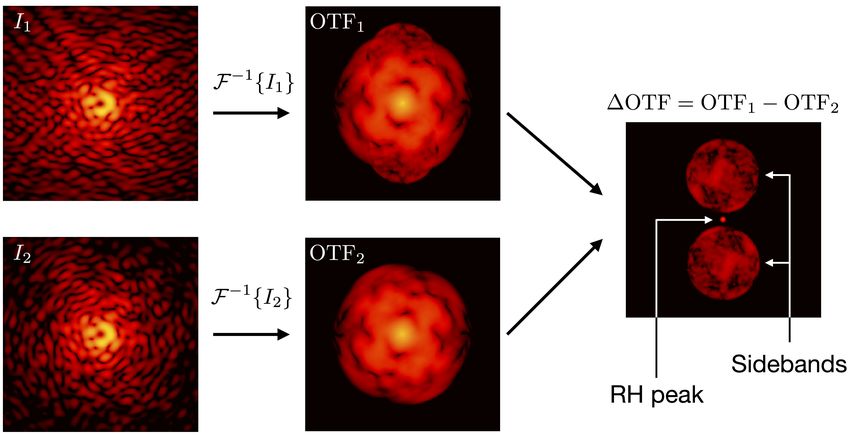
field Isb (Mazoyer et al. 2014):
Isb = F {Ep ∗ Eref
∗
}, (8)
= F {Ep }F {Eref }.
∗
(9)
This term is used with wavefront sensing and control, as shown
in Sect. 3.2. We note that Isb is a complex quantity, which
becomes completely real when the other sideband is included.
For CDI we also have to extract other information from the
∆OTF. Selecting the RH peak and calculating its Fourier trans-
form gives an estimate of the RH PSF:
Fig. 2. Example of sideband extraction with the PESCC. For the images Iref = F {Eref ∗ Eref
∗
}. (10)
of channels 1 and 2 (I1 and I2 ) in Fig. 1, the OTFs are calculated. The
OTF1 contains the two sidebands with wavefront information and the It is also important to have an estimate of the cross-talk intensity
RH peak, but these are overwhelmed by the central peak. When OTF2 , term Ict . This term can be estimated by extracting both sidebands
which only contains the central peak, is subtracted from OTF1 , the two and calculating their Fourier transform:
sidebands and RH peak are revealed.
Ict = F {Ep ∗ Eref
∗
∗ δ(x + 0 ) + Ep∗ ∗ Eref ∗ δ(x − 0 )}, (11)
= 0 ∗
2R{F {Ep }F {Eref } }. (12)
the same location as the main beam, but is much fainter than the
central peak, and is smaller with a width of 2dr . The cross-talk
between the RH beam and the central beam generates two lateral 2.2. Reference hole diameter
peaks or sidebands in the OTF located at ±0 , both with a width The diameter of the RH (dr ) directly depends on the size of
of D+dr . As the RH is placed close to the pupil (0 < D), the two the dark hole. The dark hole size is set by the maximum spa-
sidebands still partly overlap with the central peak. See Fig. 2 tial √
frequency that can be controlled by the DM and is given
for a two-dimensional example that visualizes this. To reveal the by 2Nact λ/(2D) (Mazoyer et al. 2013), with D as the diame-
sidebands, which contain the wavefront information, we subtract ter of the pupil, Nact the number of actuators along one axis
the OTF2 from OTF1 : √ in
the pupil, and λ the observed wavelength. The factor of 2 is
included to account for the higher number of actuators along the
∆OTF = Eref ∗ Eref
∗
+ Ep ∗ Eref
∗
∗ δ(x + 0 ) diagonal compared to the sides of a square grid of actuators in a
+ Ep ∗ Eref ∗ δ(x − 0 ).
∗
(7) DM. To make sure that the DM can actually remove the speckles
within the dark hole, the electric field of the speckles needs to be
accurately measured. This can only happen when the focal-plane
If 0 has been appropriately chosen (Sect. 2.3), the three remain- electric field of the RH is non-zero over the dark hole. The posi-
ing peaks in the OTF are well separated. It is essential that tion of the first dark ring of the RH PSF is located at 1.22λ/dr .
differential aberrations between the two channels are minimal, Therefore, the diameter (dr ) is given by (Mazoyer et al. 2014):
otherwise the Ep ∗ Ep∗ term does not completely cancel in the
subtraction. Extracting, centering and Fourier transforming one √ D
of the sidebands gives an estimation of the focal-plane speckle dr ≤ 1.22 2 . (13)
Nact
A177, page 4 of 16S. P. Bos: The polarization-encoded self-coherent camera
1.0
Fringe for cen
Fringe for min
Fringe for max
0.8
Normalized fringe strength
0.6
0.4
0.2
Fig. 3. Explanation of how the geometry of the pupil relates to the
geometry of the OTF. This figure shows that the minimum distance of 0.0
the RH of (a) the SCC is much larger than that of (b) the PESCC. 20 15 10 5 0 5 10 15 20
x[ cent/D]
Fig. 4. Example of fringe smearing by spectral bandwidth. Fringes are
Often, the ratio between the pupil diameter and reference hole plotted for many wavelengths within a broadband filter (Rλ = 5). All are
diameter is used, γ = D/dr . Then the Eq. (13) becomes: plotted with a period of 5 λ/D, but due to the changing wavelength the
physical fringe periods in the focal plane change as well. This results in
Nact significant fringe blurring after only a few periods from the center.
γ≥ √ . (14)
1.22 2
pupil, the sampling (S), in units of pixels (Npix ) per λ/D, is given
2.3. Reference hole distance by:
For the SCC, the minimum distance of the reference hole
(0 ) with respect to the center of the pupil was derived in Npix
S= , (17)
Galicher et al. (2010). It ensures that the sidebands would not λ/D
overlap with the central peak in the OTF (see Fig. 3a), and is
given by: with λ as the wavelength. To be Nyquist sampled in the focal-
plane, it is required that Npix ≥ 2, and is usually set to Npix = 3
β
!
1
0 = 3+ D, (15) or Npix = 4. For the (PE)SCC, the combined diameter of the
2 γ pupil and RH becomes D ⇒ D + o − D/2 + dr /2 (Fig. 3). This
results in the following sampling constraint:
with β a factor that cannot be lower than unity and usually set
to 1.1 to include some extra margin. However, for the PESCC
the sidebands can overlap with the central peak in the OTF as Npix
S= . (18)
the central peak is subtracted out. The only constraint is that the λ/[(D + dr )/2 + 0 ]
sidebands do not overlap with one another or the peak from the
RH, otherwise the wavefront information cannot be completely When substituting the value of 0 for the SCC (Eq. (15)) in this
extracted, which is shown in Fig. 3b. For the PESCC, this leads equation, we can rewrite it as:
to the following reference hole distance law:
(1 + β)(1 + 1/γ) + 2β Npix
β S= .
!
2 (19)
0 = 1+ D. (16) 2 λ/D
2 γ
Now we investigate in the ideal case how much closer the refer- For the PESCC (Eq. (16)) we find:
ence hole can be placed for the PESCC compared to the SCC.
We set β = 1 and assume an infinitely small reference hole (1 + β)(1 + 1/γ) + β/γ Npix
S= . (20)
dr → 0 (γ → ∞). We then find for the SCC (Eq. (15)) that 2 λ/D
0 = 1.5D. For the PESCC (Eq. (16)) we find 0 = 0.5D.
This means that the PESCC can be placed three times closer As in Sect. 2.3, we explore in an idealized example the gain in
to the center of the pupil than the SCC. This results in access to focal-plane sampling is for the PESCC. Again, we assume that
more light in the RH, as the focal-plane masks of coronagraphs β = 1, and that dr → 0 (γ → ∞). We set Npix to 2 pixels to meet
diffracts more light closer to the geometric pupil, and, as shown the Nyquist sampling constraint. For the SCC, we find that S = 4
in the following sections, it relaxes the focal-plane sampling con- pixels per λ/D, which means that the sampling should be twice
straints and allow for broader spectral bandwidths. as high compared to the unobscured pupil. On the other hand,
the PESCC has a sampling of S = 2 pixels per λ/D, which is
2.4. Focal-plane sampling constraints equal to the case of the unobscured pupil. This is because in this
idealized example, the RH is infinitely small and can be placed
As the RH of the PESCC can be positioned significantly closer right on the edge of the pupil. This shows that the PESCC sig-
to the pupil, the constraints on the focal-plane sampling can be nificantly relaxes the sampling requirements as the total number
relaxed. In this subsection, we investigate what the sampling of pixels on the detector can be reduced, in the ideal case, by a
constrains are for the PESCC. For an unobstructed telescope factor of four.
A177, page 5 of 16A&A 646, A177 (2021)
2.5. Spectral bandwidth limitations
Exoplanets are preferably observed over broad wavelength
ranges (∆λ) to maximize the signal-to-noise ratio (S/N). How-
ever, the PSF is not constant, changing its size with wavelength
(∝λ/D). This means that the fringes introduced by (PE)SCC also
increase their size and period with wavelength. Close to the cen-
ter of the image these chromatic effects are not that pronounced,
but after a few periods the fringes of the lowest and highest
wavelengths in the filters start to significantly shift with respect
to each other. An example of this is shown in Fig. 4. After a
certain distance from the image center the fringes are blurred
to a level that it severely impacts the wavefront sensing perfor-
mance. However, in the direction orthogonal to the fringe, the
smearing is minimal and therefore the wavefront sensing in that Fig. 5. Regions in the OTF1 and OTF1 that are not contaminated by
direction is still relatively accurate. Here, we study the band- the sidebands or the RH. Therefore, regions A and B are suitable to
width for (PE)SCC solutions with one RH. Broadband solutions measure p.
for the SCC with multiple RHs do exist (Delorme et al. 2016),
but require even larger optics than the SCC to accommodate
the additional reference beams. This is because for SCC solu- up having an equal intensity and when the ∆OTF is calculated,
tions with one DH, the constraint on the optics diameter can they will not be completely canceled out in the subtraction. We
be somewhat mitigated by moving the central pupil from the are mainly concerned with the polarization introduced by the
center of the optics. The RH beam and the main beam will telescope and instrument because starlight is generally unpolar-
then both pass through off-axis positions in the optics. How- ized (e.g., the integrated polarization signal of the Sun is 0 and fewer photons when p < 0, and therefore it will
(2010). Then, for the PESCC, we find Rλ ≈ 24. Thus, the PESCC affect the wavefront sensing sensitivity by decreasing or increas-
can operate over bandwidths that are ∼3.5 times wider than the ing the photon noise. However, as p is expected to be around
SCC. This result can be understood as follows. The period of 10−2 , this effect will have less of an impact than the residuals of
the fringes is determined by 0 : when the RH is further away the central peak.
from the pupil, the period of fringes becomes shorter. For a fixed If the value of p is known, then it is possible to compen-
spectral bandwidth the number of fringe periods before the blur- sate for its effects in post-processing by dividing OTF1 and OTF2
ring becomes too strong is also fixed. Because the PESCC has with, respectively, 1 + p and 1 − p. This removes the detri-
a smaller 0 than the SCC, the PESCC fringe periods are longer mental effects of the first term in Eq. (24), but it does not affect
and the blurring becomes too strong at larger physical distances. the sensitivity of the other terms as it cannot correct the fun-
Turning it around, when the size of the dark hole and thus the damental effects of photon noise. Much effort has already gone
distance at which the blurring can occur are fixed, the PESCC in understanding the polarization effects of high-contrast imag-
can operate over broader bandwidths than the SCC. ing instruments (De Boer et al. 2020; Van Holstein et al. 2020).
Therefore, a detailed model that describes the instrumental polar-
2.6. Instrumental polarization ization at a given configuration of the telescope and instrument
could help to mitigate these effects. It is also possible to directly
When the starlight is polarized, it is possible that the perfor- measure p in OTF1 and OTF2 . As shown in Fig. 5 by the circles A
mance of the PESCC is affected. This is because the central and B, it is possible to selection regions in the OTFs without con-
peaks in the two channels (I0 in Eqs. (1) and (2)) will not end tamination of the sidebands or the RH. By calculating the flux in
A177, page 6 of 16S. P. Bos: The polarization-encoded self-coherent camera
region A (FA ) and B (FB ), it is possible to estimate p: incoherent circumstellar environment (e.g., an exoplanet, or cir-
FA − FB cumstellar disk), the measurements in channel 1 and 2 become:
p= . (25)
FA + FB I10 = I1 + Iic , (28)
I20 = I2 + Iic , (29)
2.7. Polarization leakage
with I1 and I2 given by Eqs. (1) and (2), and Iic the incoher-
In Sect. 2.1, we assume that the RH polarizer and the PBS would ent contribution. We assume that p = 0 and t = 0. Deriving
perfectly split the two polarization states. However, polarizers the Ic term is slightly different for the two channels, as only
are not perfect and can be misaligned with respect to each other, one has the RH beam interfering. For channel 1 we find Iic as
which makes the reference beam leak from channel 1 into chan- (Galicher & Baudoz 2007):
nel 2. Channel 2 will then also form (weaker) fringes in the focal-
plane image, which results in the sidebands in the OTF. When Iic = I10 − Iref − Isb
2
/Iref − Ict , (30)
calculating ∆OTF, as in Eq. (7), these sidebands in channel 2
will remove the signal from the sidebands in channel 1, affecting with Iref given by Eq. (10), Isb given by Eq. (8), and Ict given by
the wavefront estimates. We rewrite Eq. (7) such that it includes Eq. (11). For channel 2 we find Iic as:
the polarization leakage:
Iic = I20 − Isb /Iref . (31)
1−t √
∆OTF = ∗
Eref ∗ Eref + (1 − t)· (26)
2 We note that the second channel does not contain the RH PSF,
∗
[Ep ∗ Eref ∗ δ(x + 0 ) + Ep∗ ∗ Eref ∗ δ(x − 0 )], and is therefore not affected by photon noise from this term.
These equations only hold for the perfect system. When there are
with t (0 ≤ t ≤ 1) the relative level of polarization leakage,
system inaccuracies present, the CDI performance will degrade
which simulates the extinction ratio of the polarizer as 1/t, and
significantly. However, inaccuracies such as p and t can be
the effect of a misaligned polarizer as:
accounted for in the post-processing step if the correct values
t = 2 sin2 (δθ), (27) are known. As shown in Sect. 2.6, it is possible to measure p in
with the misalignment angle δθ. Equation (26) shows that the the OTF1 and OTF2 . For t, it would have to be measured prefer-
central peak is always be subtracted out in this case, which is ably before the modified Lyot stop is installed. When correcting
not surprising because the main effect of polarization leakage is for these effects, Eqs. (30) and (31) become:
the reference beam leaking into channel 2. It also shows that √ the
Iic = I100 − Iref
0
/Iref − Ict0 ,
02 0
− Isb (32)
accuracy of the sideband estimate is now proportional to 1 − t,
effectively reducing the response of the wavefront sensor, which Iic = I200 − 0
t2 Iref − Isb /Iref
02 0
− tIct0 , (33)
will eventually lower the gain of the wavefront control loop. The
accuracy with which the flux in the reference hole can be esti- with I100 = I10 /(1 + p) and I200 = I20 /(1 − p) the images corrected
mated scales more favorably with (1 − t) and is therefore less for instrumental polarization effects, Iref 0
= Iref /(1 − t2 ), Isb
0
=
affected. When, for example, the RH polarizer has an extinction Isb /(1−t), and Ict = Ict /(1−t) the correction for polarizer leakage
0
ratio of 100:1, that is, 1/t = 100 → t = 10−2 , then the wavefront of respectively the RH beam, the intensity of the sideband, and
estimate is 90% of its true value, while the reference hole flux is the intensity of the cross-talk term.
99% of the truth. If the extinction ratio is accurately known, for
example by measurements before installing the modified Lyot
mask, this effect can be corrected for during post-processing or 3. Simulations
wavefront control. Another effect to take into account, especially In this section, we investigate the performance of the PESCC
with CDI as discussed in Sect. 2.8, is that the polarization leak- in numerical simulations, and compare it to the SCC where
age also contaminates the second channel. This introduces an relevant. The effects of photon noise, differential aberrations,
extra source of photon noise during post-processing with CDI. instrumental polarization, polarizer leakage, and spectral reso-
Therefore, although the effects on the wavefront control can lution on wavefront sensing and control are explored. The sim-
be calibrated, a high performance polarizer with low leakage is ulations are performed in Python using the HCIPy package
desirable. As discussed in Sect. 4, a prime candidate for the RH (Por et al. 2018), which includes polarization propagation with
polarizer are wire grids polarizers. These can be manufactured Jones matrices necessary for this work. We simulate an ideal-
to have an extinction ratio of 1000:1–10.000:1 (George et al. ized HCI system with static wavefront aberrations. The system
2013), which would result in t = 10−3 −10−4 . When the PBS is operates at 1550 nm and consists of a clear aperture, an ideal-
implemented as a Wollaston prism, which we foresee to be used, ized DM (e.g., no actuator cross-talk, or quantization errors) with
the extinction ratio exceeds 100.000:1 (King & Talim 1971), a 40×40 square grid of actuators located in the pupil plane, a
which is equivalent to t ≤ 10−5 and thus negligible compared to charge two vortex coronagraph, a (PE)SCC Lyot stop, a polariz-
the wire grid polarizer performance. A rotational misalignment ing beamsplitter and detector. The diameter of the pupil before
between the RH polarizer and PBS gives a polarization leakage the vortex coronagraph is 7 mm. The wavefront aberrations that
dictated by Eq. (27). For misalignments of 1◦ , 3◦ , and 5◦ , we find are looked at are induced by an out-of-plane phase aberration
t ≈ 6 × 10⁻⁴ , t ≈ 5 × 10⁻³ , and t ≈ 2 × 10⁻² , respectively. There- following a power spectral density with a power law exponent
fore, it is likely that rotational misalignments will dominate the of −3. Fresnel propagation from this plane to the pupil creates
polarization leakage. both phase and amplitude aberrations. This results in a wave-
front error (WFE) of 2.9 × 10⁻² (±8 × 10⁻³ ) λ root mean square
2.8. Coherent differential imaging (RMS), and intensity variations over the pupil of 16 (±1%) RMS
(measured over 100 random aberrations). The Lyot is undersized
In this subsection, we investigate how CDI is performed with by 1% compared to the pupil diameter. The diameter of the RH
the PESCC. If we consider adding the light of an unpolarized, is determined by Eq. (13) and for this specific system it is set to
A177, page 7 of 16A&A 646, A177 (2021)
Table 2. Simulation parameters for Sect. 3. = 10
= 20
= 50
Variable Value 10 3
= 100
PESCC limit
λ 1550 nm SCC limit
Pupil diameter 7 mm
fractional power
Aperture Clear 10 4
Coronagraph Charge two vortex
Lyot stop diameter 0.99 pupil diameter
Deformable mirror 40 × 40 actuators 10 5
β 1.1
dr 0.3 mm
γ 23.2
0 PESCC 4.2 mm 10 6
0 SCC 11.7 mm 0.4 0.6 0.8 1.0 1.2 1.4 1.6 1.8 2.0
Focal-plane sampling PESCC 2.24 pixels per λ/D 0/D
Focal-plane sampling SCC 4.39 pixels per λ/D
Fig. 6. Fractional power in the RH (ratio of the power in the RH and
total power in pupil plane before Lyot stop) as function of distance from
the center of the pupil. This was simulated using a charge two vortex
0.3 mm (γ = 23.2). The RH distance is determined by Eqs. (15) coronagraph and does not include the polarizer in the RH for the PESCC
and (16) for the SCC and PESCC respectively. For β = 1.1, the to show the total power available.
RH distance is 11.7 mm for the SCC and 4.2 mm for the PESCC.
This automatically sets the focal-plane sampling to 4.39 pixels
Residual wavefront error by photon noise
per λ/D for the SCC (Eq. (19)) and 2.24 pixels per λ/D for the
101 PESCC 1/ Np fit
PESCC (Eq. (20)). The simulation parameters are summarized
in Table 2. SCC 1/ Np fit
100 PESCC
First, we investigate the wavefront sensing performance in SCC
Residual RMS WFE [fractional ]
Sect. 3.1. Subsequently, we look into wavefront sensing and con-
10 1
trol in Sect. 3.2. Finally, we test the CDI with the PESCC in an
idealized system in Sect. 3.3. As the wavefront aberrations con-
10 2
sidered here remain static during the simulations, the conditions
and results are more representative for space-based observato-
10 3
ries. They mainly serve as proof of principle, and in a future
work, we will investigate more realistic conditions for ground-
10 4
based observatories.
10 5
3.1. Wavefront sensing 107 109 1011 1013
Photon number
In this subsection, we investigate how the wavefront sensing
capabilities of the PESCC compare to the SCC and how they Fig. 7. Photon noise sensitivity of the PESCC and SCC for wavefront
sensing. The reported photon number is the number of photons before
degrade due to various noise sources. To estimate the wave-
the coronagraph. The error bars show the 1σ deviation over the 100 ran-
front sensing performance, we calculate, from the two chan- dom
nels images, the ∆OTF as in Eq. (7) when the noise source is p wavefront aberration instances. The dashed and dotted lines show
1/ Np fits for photon numbers ≥1011 to show the regimes in which the
applied. Subsequently, we select one of the sidebands and cen- performance is photon noise-limited.
ter it. This sideband is the pupil-plane electric field convolved
with the pupil-plane RH electric field, and we consider that to
be the pupil-plane electric field estimate. Similarly, a noiseless the total power available) as function of the distance to the pupil
pupil-plane electric estimate is calculated for the same wave- center (0 /D) for various γ with a charge 2 vortex coronagraph.
front aberration. The residual RMS wavefront error, which is the We do not include the polarizer that would be installed in the
WFE common to both channels, is calculated by subtracting the RH of the PESCC to show the total power available. This figure
phase of the noiseless electric field estimate from the estimate shows that there is a greater number of photons available for
with noise, and is converted from units of radians to relative units the PESCC compared to the SCC, for example, at their respec-
of fractional λ. We simulate various levels of every noise source, tive minimum 0 (shown in the figure with the vertical, dotted
and for every level, we simulate a hundred random wavefront and dashed lines), there is a factor of ∼64 difference (factor ∼32
aberration instances. including the polarizer). However, the polarizing beamsplitter
does also split the main beam into two, which effectively halves
3.1.1. Photon noise performance the number of photons in the main beam. Therefore, the effec-
tive increase in the photon numbers is ∼16. We note that this last
As discussed in Sect. 2.3, the RH of the PESCC can be posi- sensitivity hit only applies to wavefront sensing and not for com-
tioned much closer to the pupil compared to the RH of the panion detection because in the latter case, both channels can
SCC. This provides access to a greater number of photons for be combined. To indicate the expected wavefront sensing per-
wavefront sensing as the coronagraph’s focal-plane mask scat- formance, we plot in Fig. 7 the wavefront sensing performance
ters most light close to the geometric pupil. In Fig. 6, we plot as function of the number of photons before the coronagraph.
the fractional power of the RH (ratio of the power in the RH and This figure shows that the PESCC consistently outperforms the
A177, page 8 of 16S. P. Bos: The polarization-encoded self-coherent camera
Residual wavefront error by differential aberrations Residual wavefront error by instrumental polarization
100 photon noise limit
uncorrected p
perfectly corrected p
10 1
Residual RMS WFE [fractional ]
Residual RMS WFE [fractional ]
10 1
10 2
10 3
10 2
10 4
10 5
10 3
10 6 10 5 10 4 10 3 10 2 10 1 100
10 4 10 3 10 2 10 1 p
[fractional ]
Fig. 9. Performance of the wavefront sensing with instrumental polar-
Fig. 8. RMS differential aberrations (∆φ) between the two beams down- ization effects. The error bars show the 1σ deviation over the 100 ran-
stream of the polarizing beamsplitter, and their effect on the wavefront dom wavefront aberration instances. The circles show that data points
reconstruction. The error bars show the 1σ deviation over the 100 ran- where the strength of instrumental polarization (p) was not corrected
dom wavefront aberration instances. and the triangles show the data points where p was corrected. The dot-
ted lines shows the photon noise limit, which was introduced to prevent
the residual wavefront error reaching numerical noise.
SCC by a factor of four, which √ is to be expected as the PESCC
receives ∼16 more photons ( 16 = 4). This enables the PESCC
to either achieve a sensitivity that is four times higher or run with be tightly controlled for successful operation of the PESCC. To
wavefront control loop speedpthat is a 16 times higher. The dot- put these values into perspective, SPHERE/IRDIS was built with
ted and dashed lines show 1/ Np fits (Np is the photon number) ∼6 × 10⁻³ waves of differential aberrations (Dohlen et al. 2008)
that are fitted to the data points for Np ≥ 1011 photons. When between the two beams.
the photon numbers become too low, then there are not enough
photons in the sidebands for wavefront information to be sub- 3.1.3. Instrumental polarization
tracted and the noise becomes dominated by numerical artifacts,
which explains the flattening of the data points. As the PESCC As discussed and analytically studied in Sect. 2.6, uncorrected
has access to more photons, it occurs at the lower photon num- instrumental polarization can impact the wavefront estimation
ber. For 1012 photons, the PESCC reaches aA&A 646, A177 (2021)
Residual wavefront error by polarization leakage Residual wavefront error by spectral resolution
()
10 1 100 101 PESCC
10 3 10 1 SCC
Residual RMS WFE [fractional ]
10 2
10 4
Residual RMS WFE [fractional ]
10 3
10 5
10 4
10 6
10 5
10 7
10 6
10 8
10 7
10 6 10 5 10 4 10 3 10 2 10 1 100 100 101 102 103 104
t R
Fig. 10. Performance of the wavefront sensing with polarization Fig. 11. Performance of the wavefront sensing with varying spectral res-
leakage. The error bars show the 1σ deviation over the 100 random olution (Rλ ). The error bars show the 1σ deviation over the 100 random
wavefront aberration instances. The bottom x-axis shows polarization wavefront aberration instances. The circles show the performance of the
leakage (t), and the upper x-axis shows the equivalent rotation offset PESCC and the triangles the performance of the SCC.
(δθ) between the RH polarizer and PBS. We note that the right most
data point is sampled at t = 0.81.
response matrix R is then constructed by stacking the responses
to the N modes that are controlled:
3.1.5. Spectral resolution
1 1 T
R{∆Isb } I{∆Isb }
Astronomical observations always have a finite Rλ , and, as was .. .
analytically studied in Sect. 2.5, this affects the performance R = . .. , (35)
of the PESCC. Specifically, it was determined when Eqs. (22) N
R{∆Isb N
} I{∆Isb }
and (23) are not satisfied, respectively, the SCC and PESCC,
accurate wavefront sensing in the entire control region of the DM with R{·} and I{·} the real and imaginary components. In the
is not possible. Here we simulate the effects of spectral resolu- simulations there is only one DM, which is set in a pupil-plane
tion on the wavefront sensing. The broadband effects are simu- and, therefore, we can only hope to correct for phase and ampli-
lated by sampling seven wavelengths over the wavelength range tude errors in a one-sided dark hole. Therefore, we chose a
defined by the spectral resolution, calculating the PSF for each ROI given by 5 λ/D < x < 10 λ/D and −5 λ/D < y <
wavelength, and incoherently adding the resulting PSFs. Due −5 λ/D. We use a sine/cosine mode basis to directly probe
to the spectral effects, the sidebands in the ∆OTF are smeared, this region (Poyneer & Véran 2005) to calibrate the response
affecting the wavefront information. We use the position and size matrix. The control matrix C is then calculated by inverting the
of the RH at the central wavelength to generate an aperture that response matrix using the singular-value decomposition method
is applied to the ∆OTF for wavefront sensing. In Fig. 11, the with Tikhonov regularization. In closed-loop operation for the
results of the simulation are shown. It shows thatS. P. Bos: The polarization-encoded self-coherent camera
Channel 1
Channel 2 Pre-WFC PSF Post-WFC PSF Blocked reference hole
Fig. 12. WFC example with the PESCC without noise sources present. The subfigures in the two rows show the PSFs of the two channels. The
columns show, respectively, the PSFs before WFC, the PSFs after twenty iterations of the WFC, and the PSFs after the WFC with the RH blocked.
The colorbar shows the intensity in logarithmic scale and is equal for all subfigures.
Raw contrast in ROI without noise Raw contrast in ROI with photon noise
10 5 channel 1 10 5 channel 1, Np = 108 channel 2, Np = 1010
channel 2 channel 2, Np = 108 channel 1, Np = 1012
channel 1, Np = 1010 channel 2, Np = 1012
10 6 10 6
1 raw contrast
1 raw contrast
10 7
10 7
10 8
10 8
10 9
10 9 2.5 5.0 7.5 10.0 12.5 15.0 17.5 20.0
2.5 5.0 7.5 10.0 12.5 15.0 17.5 20.0 Iteration
Iteration
Fig. 14. Raw contrast as function of iterations for the system with pho-
Fig. 13. Raw contrast as function of iterations in the ROI for WFC ton noise. The response matrix is acquired without photon noise. At
example with noise sources. At iteration 21, the RH is blocked to show iteration 21, the RH is blocked to compare the raw contrasts in the two
that the dark holes reach similar raw contrasts. channels.
3.2.2. Differential aberrations
observing a very bright source (e.g., an internal source within the
instrument) such that photon noise is irrelevant, that is, we did As shown in Sect. 3.1.2, differential aberrations between the
not simulate photon noise while acquiring the response matrix. two beams after the PBS severely affect the wavefront sens-
In Fig. 14, the results are presented. For 108 photons per expo- ing. Here, we quantify to what level it limits the WFC. When
sure the wavefront control converges to ∼4 × 10⁻⁸ contrast. With calibrating the response matrix, the differential aberrations are
1010 photons, the contrast is close to that of the perfect system, at included as they are expected to be always present in the sys-
∼3 × 10⁻⁹ . Then for 1012 photons, the contrast that is reached is tem. In Fig. 15, the convergence of the WFC under various
that of the perfect system, ∼2 × 10⁻⁹ . When considering the cur- levels of differential aberration is shown. For ∆φ = 10−2 λ,
rent internal near-infrared (NIR) camera and ∆λ = 50 nm filter the PESCC converges to a contrast of ∼4 × 10⁷ . With ∆φ =
at 1550 nm in SCExAO (Jovanovic et al. 2015; Lozi et al. 2018), 6 × 10⁻⁴ λ it converges close to the benchmark performance at
which is located at the 8 meter Subaru telescope on Maunakea, ∼3 × 10⁻⁹ contrast. For ∆φ = 2 × 10⁻⁵ λ the system converges
these photon numbers correspond to ∼2 Hz WFC loop speed on to the benchmark system results at ∼2 × 10⁻⁹ . To put these val-
a mH = 6, mH = 1, and mH = −4 target, respectively. ues into perspective, the SCExAO/CHARIS polarization mode
A177, page 11 of 16A&A 646, A177 (2021)
Raw contrast in ROI with differential aberrations age in the response matrix calibration. The results presented in
10 5 channel 1, = 1 10 2 channel 2, = 6 10 4 Sect. 3.1.4 show that the wavefront error is never affected more
channel 2, = 1 10 2 channel 1, = 2 10 5 than on the level of a 10−4 fractional λ RMS WFE. Therefore,
channel 1, = 6 10 4 channel 2, = 2 10 5 we decided to test t = 10−2 , 10−4 , 10−6 . The results are shown
in Fig. 17. It shows that for t = 10−3 , the contrast in channel 2
10 6
initially does not converge to the benchmark contrast. When the
1 raw contrast
RH is blocked, then both channels converge to ∼2 × 10⁻⁹ , which
shows that channel 2 was limited by leakage from the RH PSF.
10 7
This proves that the WFC itself is not limited by polarizer leak-
age, but that the contrast in the DH could be limited by leakage
from the polarizer. As discussed in Sect. 2.7, polarization leak-
10 8
age is expected to be t = 10−3 −10−4 , and t ≤ 10−5 for the RH
polarizer and PBS, respectively, and are not expected to to have
an impact on WFC. When the RH polarizer and PBS are mis-
10 9 aligned by 5◦ the leakage is ∼2 × 10⁻² , which is also on a level
2.5 5.0 7.5 10.0 12.5 15.0 17.5 20.0 that does not impact the WFC, but the contrast in channel 2 will
Iteration
then be limited by RH PSF to ∼7 × 10⁻⁹ .
Fig. 15. Raw contrast as function of iterations for the system with dif-
ferent levels of RMS differential aberrations (∆φ) between the beams.
The response matrix is acquired with the differential aberrations present. 3.2.5. Spectral resolution
At iteration the RH is blocked to compare the raw contrast in the two
channels. Here, we simulate the effects of spectral resolution on WFC.
The broadband effects are included when the response matrix
is measured and the wavefront measurements are identical to
(Lozi et al. 2019) has ∼7 × 10⁻³ waves of differential aberra- Sect. 3.1.5. Similarly as before, we sample seven wavelengths
tions1 , and SPHERE/IRDIS was built with ∼6 × 10⁻³ waves of of the spectral band and add the resulting PSFs to get the broad-
differential aberrations (Dohlen et al. 2008) (both values calcu- band PSF. In Fig. 18, we show the WFC results for various Rλ .
lated at λ = 1600 nm). This means that if PESCC were imple- It shows that for Rλ = 8, the WFC control diverges and that the
mented at either of these systems, it would converge to a 1σ raw
contrast in the ROI becomes worse. For Rλ = 30 and Rλ = 100,
contrast between ∼4 × 10⁷ and ∼3 × 10⁻⁹ , probably closer to the
former. the WFC converges (close) to the contrast achieved by the sys-
tem without noise sources. The tested spectral resolutions are
equivalent to filters with bandwidths of 0.13 · λ0 , 0.03 · λ0 , and
3.2.3. Instrumental polarization 0.01 · λ0 . Therefore, as shown in Fig. 18, the PSECC does not
Here, we test the effect of (un)corrected instrumental polariza- work with the broadband photometric filters, but with narrow-
tion on the WFC with the PESCC. When calibrating the response band filters that have δλ ≤ 0.03 · λ0 it will be able to run a
matrix the instrumental polarization effects are included when WFC effectively. Operation of the PESCC with an integral field
there is no correction of p in post-processing. When the instru- spectrograph (IFS) would be an ideal solution as it provides
mental polarization is corrected, the correction is also included relatively narrowband images over broad wavelength ranges.
when calibrating the response matrix. In Fig. 16a we show the SCExAO/CHARIS (Groff et al. 2017) offers a low-resolution
WFC results when the instrumental polarization is not corrected. mode at Rλ = 18 and high-resolution modes at Rλ ≈ 70. The
For p = 3 × 10⁻² , the loop is not stable because the contrast PESCC is able to operate with the high-resolution modes. And
first increases, and then decreases. The final contrast achieved is SPHERE/IFS operates either with Rλ = 30 (Claudi et al. 2008)
∼4 × 10⁻⁶ , which is only a slight improvement from the initial or Rλ = 50 (Mesa et al. 2015), which means that the PESCC can
contrast. When p = 2×10⁻³ , the system converges to ∼10−8 con- operate with both modes.
trast. Then, for p = 1.3 × 10⁻⁴ the contrast achieved is ∼2 × 10⁻⁹ ,
equal to the benchmark results.
In Fig. 16b the polarization effects are corrected during WFC 3.2.6. Combined effects
by the method presented in Sect. 2.6. It shows that for all cases,
the WFC converges to the contrast of the system without noise. Here, we combine the tested noise sources in one simulation to
Uncorrected instrumental polarization at SPHERE/IRDIS is at a investigate whether these noise sources interact with each other.
level of p ≈ 10−2 , and when corrected, using a detailed instru- For every noise source, we select the level that gives a 10−2 λ
ment polarization model, reaches p ≤ 10−3 (Van Holstein et al. WFE, as described in Sect. 3.1. All the noise sources, except the
2020). As shown in the results of Fig. 16a, this means that the photon noise, are included when calibrating the response matrix.
instrumental polarization have to be corrected as, otherwise, the During the wavefront sensing step, the instrumental polarization
loop would be unstable and diverge. When the instrument polar- is measured and corrected in the frames. The results are pre-
ization model is used and p is corrected to a level of ∼10−3 , then sented in Fig. 19. This shows that the WFC control converges
the WFC will converge to ∼10−8 contrast. to a contrast of ∼10−8 , which is very similar to the raw contrast
achieved when there were uncorrected p effects at p ∼ 2 × 10⁻³ ,
roughly an order of magnitude worse than the performance under
3.2.4. Polarization leakage the other individual noise sources. This is caused by the differ-
We investigate the effects of polarizer leakage on the WFC. As ential aberrations, which introduce intensity differences between
with the previous subsections, we include the polarizer leak- the OTFs of the two channels at locations where p is measured.
These intensity differences are not caused by p effects and, there-
1
As derived from a Zemax file provided by T. Groff. fore, lead to incorrect p estimates.
A177, page 12 of 16S. P. Bos: The polarization-encoded self-coherent camera
a) b)
Fig. 16. Raw contrast as function of iterations for the perfect system with instrumental polarization (p) effects. At the last iteration, the RH is
blocked to compare the raw contrast in the two channels. Panel a: during the acquisition of the response matrix and the closed loop tests the effects
of p were not corrected. Panel b: during all steps of the response matrix acquisition and WFC tests, p was corrected. All three tested levels of p
now overlap and reach the performance level of the benchmark tests.
Raw contrast in ROI with polarization leakage Raw contrast in ROI with spectral resolution
10 5 channel 1, t = 10 2
10 5
channel 2, t = 10 2
channel 1, t = 10 4
channel 2, t = 10 4 channel 1, R = 8 channel 2, R = 30
10 6 channel 1, t = 10 6 10 6 channel 2, R = 8 channel 1, R = 100
channel 2, t = 10 6 channel 1, R = 30 channel 2, R = 100
1 raw contrast
1 raw contrast
10 7 10 7
10 8 10 8
10 9 10 9
2.5 5.0 7.5 10.0 12.5 15.0 17.5 20.0 2.5 5.0 7.5 10.0 12.5 15.0 17.5 20.0
Iteration Iteration
Fig. 17. Raw contrast as function of iterations for the system with polar- Fig. 18. Raw contrast as function of iterations for the system with broad-
izer leakage. The response matrix is acquired with the polarizer leakage. band effects. The response matrix is acquired with the broadband effects
At iteration 21, RH is blocked to compare the raw contrast between the included. At iteration 21, the RH is blocked to compare the raw contrast
two channels. in the two channels.
Raw contrast in ROI with the combined noise sources
3.3. Coherence differential imaging 10 5 channel 1
channel 2
In this subsection, we study the improvements in contrast that
CDI could bring with the PESCC, which was developed in
10 6
Sect. 2.8. As proof of principle, we simulate a monochromatic,
1 raw contrast
idealized system without any noise sources other than wavefront
aberrations. The parameters as presented in Table 2 are used 10 7
for the simulation. We compare the CDI before and after the
WFC. We aim to minimize the starlight in the ROI, defined by
1 λ/D > r > 18 λ/D and x > 0. The ROI is larger than what 10 8
was used in Sect. 3.2 to show that the PESCC is not limited to a
dark hole size. Unlike in Sect. 3.2, we do not block the RH after
the final WFC step. This is to estimate the effect of subtracting 10 9
the terms involving the RH PSF. In Fig. 20, the PSFs are shown 2.5 5.0 7.5 10.0 12.5 15.0 17.5 20.0
Iteration
before and after the WFC as well as after the CDI. It shows that
the WFC improves the contrast in the ROI, as it is intended to do, Fig. 19. Raw contrast as function of iterations for the system with all
while the CDI improves the entire FOV. Furthermore, it shows effects. The response matrix is acquired with all effects included. At
that CDI is not able to completely remove the PSF and bring the iteration 21, the RH is blocked to compare the raw contrasts in the two
contrast to numerical noise. This is likely due to numerical arti- channels.
facts. The PSF of the RH is clearly visible in the post-WFC PSF
of channel 1, and is largely removed after the final CDI step. A and ∼10−6 . When performing CDI on the initial PSFs, the con-
radial profile of the contrast in the ROI is shown in Fig. 21. It trast is improved to ∼6×10⁻⁸ −3×10⁻⁹ , which is an increase of a
shows that the initial contrast in the ROI is between ∼4 × 10⁻⁴ factor of ∼330−6600. Following the WFC, the contrast becomes
A177, page 13 of 16You can also read